DenseNet-Based Classification of EEG Abnormalities Using Spectrograms

Abstract

Electroencephalogram (EEG) analysis is essential for diagnosing neurological disorders but typically requires expert interpretation and significant time. Purpose: This study aims to automate the classification of normal and abnormal EEG recordings to support clinical diagnosis and reduce manual workload. Automating the initial screening of EEGs can help clinicians quickly identify potential neurological abnormalities, enabling timely intervention and guiding further diagnostic and treatment strategies. Methodology: We utilized the Temple University Hospital EEG dataset to develop a DenseNet-based deep learning model. To enable a fair comparison of different EEG representations, we used three input types: signal images, spectrograms, and scalograms. To reduce dimensionality and simplify computation, we focused on two channels: T5 and O1. For interpretability, we applied Local Interpretable Model-agnostic Explanations (LIME) and Gradient-weighted Class Activation Mapping (Grad-CAM) to visualize the EEG regions influencing the model’s predictions. Key Findings: Among the input types, spectrogram-based representations achieved the highest classification accuracy, indicating that time-frequency features are especially effective for this task. The model demonstrated strong performance overall, and the integration of LIME and Grad-CAM provided transparent explanations of its decisions, enhancing interpretability. This approach offers a practical and interpretable solution for automated EEG screening, contributing to more efficient clinical workflows and better understanding of complex neurological conditions.

1. Introduction

Electroencephalogram (EEG) is a important tool that assists in the analysis of various neurological disorders, including epilepsy, Parkinson’s disease, and Alzheimer’s disease [1]. By recording electrical activity in the brain, EEG provides valuable insights into the brain’s functioning and helps in the diagnosis and monitoring of these conditions. The classification of EEG signals into normal and abnormal patterns is a fundamental first step in this analysis [2], as it enables clinicians to identify potential abnormalities that may indicate underlying neurological issues. This classification not only facilitates timely intervention but also guides treatment decisions, ultimately improving patient outcomes and advancing our understanding of these complex diseases.

Previous research on EEG-based event classification methods has relied on estimating features from the time, frequency, and time–frequency domains, which are then used as inputs for machine learning algorithms [3,4]. This approach requires a solid background in signal processing, and the performance of these models heavily depends on the quality of the estimated features.

In response, deep learning methods have been introduced to classify EEG events without the need for manual feature extraction [5,6,7]. However, these techniques require large EEG datasets for training to achieve high performance. Additionally, complex deep-learning architectures demand substantial training time and computational resources [8]. Transfer learning has emerged as a viable solution, allowing researchers to leverage pre-trained weights to address these challenges [9]. Consequently, more researchers [10,11,12] are adopting transfer learning methods to analyze EEG events.

Despite advancements in artificial intelligence techniques for EEG analysis that enhance performance, the interpretability of these methods has become increasingly challenging [13]. Explainability is particularly crucial in the medical domain, where understanding model decisions can significantly impact patient care [14]. Techniques such as SHapley Additive exPlanations (SHAP) [15], Local Interpretable Model-agnostic Explanations (LIME) [16] and Gradient-weighted Class Activation Mapping (Grad-CAM) [17] have been proposed to improve the interpretability of these models and enhance our understanding of their decision-making processes.

The Temple University Hospital Abnormal EEG Dataset (TUAB) [18] was created from archived records at Temple University Hospital and is regarded as the largest publicly available collection of clinical EEG recordings worldwide [19]. The TUAB dataset has been annotated as either normal or abnormal and has been widely utilized in various studies [20,21,22,23,24,25] to develop methods for classifying abnormal EEG signals.

Channels T5 and O1 are often chosen in TUAB EEG tasks [20,23], because they provide critical information about temporal and occipital brain activity, regions commonly involved in pathological conditions like epilepsy and encephalopathy [19]. Channel T5 located in the left temporal lobe, is sensitive to abnormalities such as spikes and sharp waves [26], while channel O1, in the left occipital region, detects patterns like occipital slowing or periodic discharges. These channels are less prone to artifacts from eye movements compared to frontal channels [27,28], making them ideal for identifying abnormalities with higher sensitivity and signal quality. Therefore, channels T5 and O1 were chosen as inputs in this study for classifying normal and abnormal EEGs in the TUAB dataset [20,23].

Signal images, spectrograms, and scalograms are commonly used for EEG event analysis, providing insights from various domains. To ensure a fair comparison among these EEG representations, we evaluated their performance under consistent model settings. To improve performance with limited data and to reduce computational costs, we used these representations as input to a DenseNet transfer learning-based strategy, with post-processing applied across multiple images. To enhance model interpretability, we used LIME and Grad-CAM techniques, which visualize the regions of the input data most influential to the predictions, enabling researchers to gain a clearer understanding of the model’s decision-making process. Using only channels T5 and O1 of the TUAB EEG data our method obtained results comparable to multi-channel models for classifying normal and abnormal EEG signals. The main contributions of this study are as follows:

• Presents a transfer learning model for automated classification of EEG recordings as normal or abnormal, enabling high-throughput screening in clinical workflows. This facilitates early identification of potential neurological abnormalities, allowing clinicians to focus on abnormal EEGs, support timely intervention, and improve diagnostic efficiency and patient outcomes.
• Presents an EEG classification approach that achieves competitive performance using only two channels (T5 and O1), thereby reducing computational complexity and wiring requirements compared to full multi-channel models.
• Explores signal images, spectrograms, and scalograms as complementary representations of EEG signals, and compares their effectiveness in capturing features relevant to abnormal EEG detection across the time, frequency, and time–frequency domains.
• Applies a DenseNet-based transfer learning strategy to enhance model performance with limited EEG data and minimize the need for training deep networks.
• Implements a post-processing approach across multiple image representations to further improve classification performance.
• Incorporates explainable AI techniques (LIME and Grad-CAM) to visualize the most influential regions of input data, thereby improving the interpretability and transparency of the model’s decision-making process.

While several studies have explored deep learning for EEG analysis, relatively few have combined DenseNet-based transfer learning with signal images, spectrograms, and scalograms for abnormality detection using only two channels. By integrating lightweight representations, an efficient model architecture, and explainable AI techniques, this work contributes a novel and practical approach to interpretable, low-complexity EEG classification, well suited for real-world clinical applications where computational and interpretability constraints are important.

2. Related Work

Previous methods for TUAB EEG normal abnormal classification have predominantly focused on feature extraction techniques [20] and deep learning models [23,29]. Some studies [30,31] trained and tested models on the same patient data, without evaluating performance on unseen datasets. Additionally, many classification approaches [20,25] used only the first 60 s of EEG recordings or excluded this period due to artifacts [31], potentially limiting their generalizability to full EEG recordings or other datasets. Furthermore, many deep learning-based methods lack interpretability, which can lead to distrust from researchers.

Despite the widespread use of the TUAB dataset, existing studies vary considerably in preprocessing pipelines, channel selection, model design, and the amount of EEG data utilized.

Table 1. Comparison of existing studies using the TUAB dataset for EEG classification.

	Model Type	Channels	EEG Duration	Accuracy
[31]	Deep neural networks	21	<15 min	86.16%
[2]	ChronoNet (RNN)	All	First 1 min	86.57
[30]	CLBP + SVM	24	First 1 min	93.84–98.19%
[20]	KNN/RF	T5–O1	First 1 min	58.2% (KNN), 68.3% (RF)
[23]	CNN	T5–O1	First 1 min	79.34%
[29]	WaveNet + LSTM	T5–O1	First 30 s	88.76%
[21]	CNN	All	Up to 11 min	76.90%
[32]	Deep Learning	All	Up to 20 min	RMSE: 0.47–1.75

provides a structured comparison of representative studies, highlighting these methodological differences.

As shown in Table 1, previous studies demonstrate substantial variability in their use of TUAB EEG data, particularly in terms of selected channels and recording duration. To address these inconsistencies, our study utilizes the full-length EEG recordings and evaluates performance on an independent test set to ensure robust and generalizable results.

3. Methodology

3.1. Dataset

The TUAB dataset is divided into two folders: training sessions and test sessions, containing a total of 2993 EEG recordings collected at sampling frequencies of 250 Hz, 256 Hz, and 512 Hz. For this study, we excluded all recordings sampled at 256 Hz (189 files) and 512 Hz (18 files), retaining only the 2786 recordings with a sampling frequency of 250 Hz. Integrating data with varying sampling rates would have required downsampling the 256 Hz and 512 Hz recordings to 250 Hz, a process that may introduce inconsistencies, particularly in time-frequency representations such as spectrograms and scalograms, which are highly sensitive to sampling rate differences. Such discrepancies can degrade feature quality and negatively impact model training and performance. To ensure consistency across the dataset and facilitate reliable feature extraction, only recordings originally sampled at 250 Hz were included in the analysis.

Among these, 2518 recordings are from the training session folder and 268 from the test session folder. The training data were further split into a training set (80%, n = 2015) and a validation set (20%, n = 503). All 268 recordings in the test session folder were used as an independent test set to evaluate the performance of the proposed method. There is no overlap between the patients in the training and test sets. To avoid any potential data leakage, the test set was not used at any stage of model development or hyperparameter tuning. Furthermore, all preprocessing steps were performed using parameters computed solely from the training data, not from the full dataset.

3.2. Data Preprocessing

To reduce artifacts and enhance signal quality, a Butterworth filter (an infinite impulse response filter) was applied to obtain the frequency band of interest (0.1–100 Hz; delta, theta, alpha, beta, and gamma wave) in the TUAB EEG recordings. Additionally, a notch filter was used to remove powerline interference at 60 Hz. For classification of normal and abnormal EEGs in the TUAB dataset, channels T5 and O1 were selected as input, providing a minimal yet informative representation while reducing data dimensionality.

The EEG recordings used in this study are labelled at the file level as either normal or abnormal, without annotations indicating the precise timing or spatial location of abnormal events within each recording. This presents a fundamental challenge for training a classification model, as a label of “abnormal” does not imply that the entire EEG trace is abnormal; many abnormal-labelled EEGs contain long stretches of normal brain activity. Training on full-length recordings without accounting for this could introduce significant label noise and degrade model performance.

To address this issue and better align the input data with the provided labels, we segmented each EEG recording into 5 min non-overlapping epochs. This epoch length reflects a strategic compromise: it is sufficiently long to capture a representative temporal context and allow for the manifestation of clinically relevant EEG patterns (e.g., seizure discharges, slowing, or asymmetries), yet short enough to minimize the inclusion of extensive normal segments in recordings labelled as abnormal. In practice, 5 min windows improve the likelihood that at least part of each segment in an “abnormal” file contains diagnostically useful activity, thereby reducing the risk of mislabeling during model training.

Moreover, shorter segments would increase the number of training samples but might miss important temporal dependencies, while much longer segments could introduce redundant or irrelevant information, increase computational demands, and hinder real-time applicability. Each 5 min epoch was then transformed into three complementary representations: signal images, spectrograms, and scalograms—to capture time-domain, frequency-domain, and time–frequency characteristics, respectively, for robust classification.

3.2.1. Signal Images

EEG signal images are extensively used in event classification tasks and have become an essential tool in fields such as clinical diagnostics, neuroscience, and brain–computer interface development [33]. In this study, 5 min EEG signal images served as input to the transfer learning model (See Figure 1 ’Signal image’). These signal images display the EEG signals from channels T5 and O1, with the X-axis representing time (0 to 5 min) and the Y-axis showing the amplitude (−0.0003 $\mathsf{\mu }$V to 0.0003 $\mathsf{\mu }$V), which corresponds to the voltage fluctuations of the EEG signal.

3.2.2. Spectrograms

Spectrograms are time-frequency representations that provide insights into frequency variations over time, making them particularly useful for detecting EEG changes during events such as epileptic seizures [12]. Figure 1 ’Spectrogram’ shows an example of the spectrogram used in this study. The X-axis in spectrograms represents time (0 to 5 min), while the Y-axis represents frequencies between 0.1 and 100 Hz. The color intensity indicates the power or magnitude of each frequency component at a given time, with hotter colors (red, yellow) showing higher power and cooler colors (blue, green) indicating lower power.

The spectrogram is generated by computing the Fast Fourier Transform (FFT) of short overlapping segments of the signal. The mathematical formula for the STFT is as follows:

1. 

Short-Time Fourier Transform (STFT):

$$X(t,f)={\int }_{-\infty }^{\infty }x\left(\tau \right)w(t-\tau )e^{-j2\pi f\tau }d\tau$$

(1)

where:

• $x\left(t\right)$ is the signal in the time domain.
• $w(t-\tau )$ is the window function (in this case, a Hamming window).
• f is the frequency.
• t is the time index for the center of the window.

• Hamming Window Function:

$$w\left(t\right)=0.54-0.46cos\left({\displaystyle \frac{2\pi t}{N-1}}\right)$$

(2)

where:

• N is the length of the window.
• t is the time index within the window.

3. 

Spectrogram:

The spectrogram is the squared magnitude of the STFT:

$$\mathrm{Spectrogram}(t,f)={\left|X(t,f)\right|}^2$$

(3)

3.2.3. Scalograms

Scalograms, derived from the continuous wavelet transform (CWT), have gained attention for their ability to capture temporal variations in EEG signals, making them highly effective for distinguishing time-frequency features of various brain events [34]. In scalograms, the X-axis represents time (0 to 5 min), while the Y-axis reflects wavelet scales that correspond to different frequency bands (0.1 and 100 Hz). The color intensity, which represents the magnitude of wavelet coefficients, highlights the strength of specific frequency components at particular times, offering a detailed view of EEG signal variations.

The scalogram using the continuous wavelet transform (CWT), which is applied to each EEG epoch (after preprocessing and filtering).

1. 

Continuous Wavelet Transform (CWT):

$$W_x(a,b)={\int }_{-\infty }^{\infty }x\left(t\right){\psi }^{\ast }\left({\displaystyle \frac{t-b}{a}}\right)dt$$

(4)

where:

• $x\left(t\right)$ is the EEG signal.
• $\psi \left(t\right)$ is the mother wavelet.
• a is the scale parameter.
• b is the translation parameter.

2. 

Morlet Wavelet (Complex Morlet Wavelet):

$$\psi \left(t\right)={\pi }^{-{\displaystyle \frac{1}{4}}}{e}^{i2\pi f_{0}t}{e}^{-{\displaystyle \frac{t^2}{2{\sigma }^2}}}$$

(5)

where:

• $f_0$ is the central frequency of the wavelet.
• $\sigma$ controls the width of the wavelet in time.

3. 

Scale and Frequency Relation: The scale a is related to the central frequency $f_0$ and $\sigma$ as:

$$a={\displaystyle \frac{1}{2\pi f_0\sigma }}$$

(6)

The corresponding frequency for each scale is given by:

$$f\left(a\right)={\displaystyle \frac{f_0}{a}}$$

(7)

4. 

Scalogram:

The scalogram is the absolute value of the CWT coefficients:

$$\mathrm{Scalogram}(t,f)=|W_x(a,b)|$$

(8)

Figure 1 illustrates examples of the signal image, spectrogram, and scalogram used in this study.

3.3. Model Development

DenseNet121 is a convolutional neural network architecture that utilizes dense connections between layers, where each layer is connected to all subsequent layers in a feed-forward manner [35]. This structure helps mitigate the vanishing gradient problem, resulting in several benefits: it reduces the training complexity of deep learning models, enables the reuse of features, and decreases the number of parameters compared to other architectures [36]. DenseNet121 is widely used for image classification tasks, particularly in medical image analysis, as it can achieve high accuracy with fewer parameters, making it suitable for solving complex medical classification challenges [37].

In this study, signal images, spectrogram and scalogram serve as inputs separately. We utilize the DenseNet121 architecture pre-trained on ImageNet as a feature extractor for EEG-based classification tasks. We exclude the top fully connected layers of the DenseNet121 model, allowing fine-tuning of the model for normal and abnormal classification.

Table 2. Input and output features used in the model.

Feature Type	Description	Data Format	Purpose
Signal Images	Raw EEG signal converted to time-domain images	2D images	Capture temporal EEG patterns
Spectrograms	Time-frequency representation of EEG signals	2D images	Capture frequency changes over time
Scalograms	Time-frequency representation using wavelets	2D images	Capture localized time-frequency features
Output	EEG classification label	Binary label (Normal/Abnormal)	Identify EEG abnormality status

shows the input and outputs of our study.

To improve the model’s adaptability to the task, we unfreeze the last 10 layers of DenseNet121, making them trainable while keeping the earlier layers frozen to retain pre-learned ImageNet features, followed by three fully connected layers with 128, 64, and 32 units, respectively, each using ReLU activation and L2 regularization (0.005) to prevent overfitting. The final output layer consists of a single neuron with a sigmoid activation function for normal and abnormal classification.

The model is compiled with the Adam optimizer with a learning rate of 0.01, and the loss function is binary cross-entropy, which is appropriate for the binary classification task. The performance is evaluated using accuracy, recall, and precision. To prevent overfitting and ensure optimal model performance, early stopping (patience = 20) is implemented, monitoring validation loss, while a model checkpoint is used to save the best-performing model based on validation accuracy. The model is trained for up to 100 epochs using the training and validation datasets.

Table 3. Hyperparameters used for model training and validation.

Hyperparameter	Value	Justification
Base Model	DenseNet121 (pre-trained on ImageNet)	Provides strong feature extraction capability from image-based EEG representations
Trainable Layers	Last 10 layers unfrozen	Allows task-specific fine-tuning while preserving general visual features from ImageNet
Top Layers	Three dense layers (128, 64, 32 units)	Adds task-specific nonlinearity and representation capacity
Activation Function	ReLU (for hidden layers), Sigmoid (for output)	ReLU prevents vanishing gradient; Sigmoid suitable for binary classification
Regularization	L2 = 0.005	Helps prevent overfitting by penalizing large weights
Loss Function	Binary Cross-Entropy	Appropriate for binary classification (normal vs. abnormal)
Optimizer	Adam	Adaptive learning rate, widely used and effective for deep networks
Learning Rate	0.01	Empirically chosen to balance convergence speed and stability
Early Stopping	Patience = 20 (monitoring validation loss)	Stops training when performance no longer improves to avoid overfitting
Model Checkpoint	Best model saved by validation accuracy	Ensures optimal model selection during training

shows the hyperparameters used for model training and validation.

3.4. Post-Processing

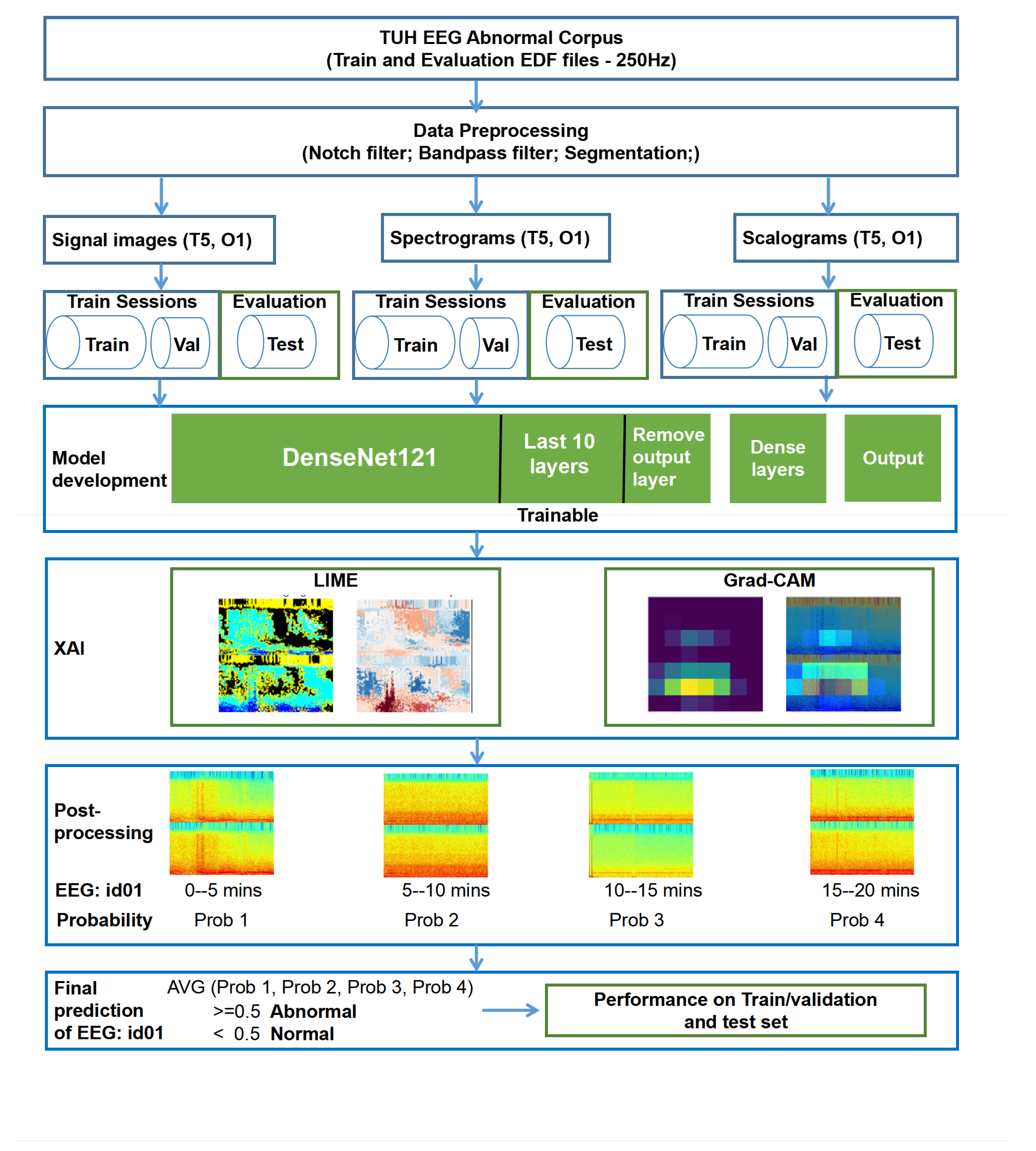
We combine the predictions from multiple image outputs by averaging them to obtain the final prediction. A full EEG recording typically lasts around 20 min (see

Table 4. Number and duration of the TUAB EEGs used in the training, validation, and test set.

	Normal	Abnormal	Total
Train	1045	970	2015
Duration/file (mins)	20.50	20.37	20.44
Duration (mins)	21,425	19,760	41,185
Validation	261	242	503
Duration/file (mins)	20.06	20.91	20.47
Duration (mins)	5235	5060	10,295
Test	148	120	268
Duration/file (mins)	20.17	20.79	20.45
Duration (mins)	2985	2495	5480

), and we used a 5 min segment. Therefore, each EEG file produces approximately three to five images. The final prediction for each EEG file is made by calculating the average of the prediction probabilities across all images generated from that file. Figure 2 shows the flowchart of the proposed method.

Let $n_i$ represent the number of images generated from EEG file i, where $n_i\in [3,5]$.

For each image j from EEG file i, let $p_{ij}$ denote the prediction probability.

The final prediction $P_i$ for EEG file i is calculated as the average of the prediction probabilities across all images:

$$P_i={\displaystyle \frac{1}{n_i}}\sum _{j=1}^{n_i}{p}_{ij}$$

(9)

The performance of the model is evaluated based on these final predictions.

3.5. Explainable Methods

In this section, we present the visualisation and interpretability methods used in our study. Specifically, LIME and Grad-CAM, which are introduced in Section 3.5.1 and Section 3.5.2, respectively, are employed to interpret the model’s predictions.

3.5.1. Local Interpretable Model-Agnostic Explanations

In this study, the LIME technique was used to interpret the model’s predictions [16]. LIME was specifically applied to generate explanations for the classification results by creating perturbed versions of the input image and assessing their impact on the model’s predictions. The process involves preprocessing the input image, performing model inference, explaining the model’s prediction through LIME, followed by the visualization of the explanation using heatmaps.

a. 

Image Preprocessing

Given an input EEG spectrogram I of shape $(H,W,C)$, where H represents the height, W the width, and C the number of channels, the image is resized to match the model’s input dimensions of $224\times 224\times 3$.

b. 

Model Prediction

The pre-trained DenseNet121 model, denoted as $f_{\mathrm{DenseNet}}$, is used to perform the inference. Given the input image ${\mathbf{I}}_{\mathrm{batch}}$, the model outputs a probability vector $\mathbf{p}=[p_1,p_2,\dots ,p_K]$, where K is the number of classes. In our binary classification task, $K=2$, corresponding to class 0 (normal) and class 1 (abnormal).

The predicted class $\widehat{y}$ is defined as the class with the highest predicted probability:

$$\widehat{y}=arg\underset{i\in \{1,\dots ,K\}}{max}{p}_i$$

(10)

The corresponding predicted probability, or confidence score, is defined as:

$$a=p_{\widehat{y}}=max\left(p_i\right),i=1,\dots ,K$$

(11)

This confidence score a indicates how certain the model is in its prediction and is used later as a reference value when interpreting the impact of individual superpixels in the LIME explanation. Specifically, higher confidence allows more robust interpretation of which regions most strongly contributed to the final decision.

c. 

Model Explanation using LIME

To interpret the model’s prediction, we apply Local Interpretable Model-agnostic Explanations (LIME), a technique that approximates the black-box model with a surrogate interpretable model. Let x represent the input image, and $\mathcal{E}\left(x\right)$ represent the explanation for x, which can be formally written as:

$$\mathcal{E}\left(x\right)=arg\underset{\mathcal{M}}{min}\mathcal{L}(f,\mathcal{M},x)$$

(12)

where:

• $\mathcal{M}$ is a simple interpretable model (e.g., linear regression or decision tree),
• $\mathcal{L}$ is the loss function that measures the fidelity of $\mathcal{M}$ to the original model f,
• f is the black-box model (DenseNet121),
• x is the input image.

LIME generates explanations by perturbing the input image and training a local surrogate model on these perturbed samples. The explanation is provided in the form of a set of superpixels, which are small regions of the image that are interpreted to be meaningful features.

d. 

Superpixel Mask and Heatmap Generation

LIME assigns a weight $w_i$ to each superpixel $x_i$ to indicate its contribution to the model’s decision. The local explanation for a given class c can be represented as:

$$\mathrm{Explanation}\left(x\right)=\sum _{i\in M}{w}_i{x}_i$$

(13)

where M denotes the set of superpixels, and $x_i$ is the feature corresponding to superpixel i. The explanation weight $w_i$ quantifies the importance of each superpixel in the model’s decision. Superpixels are obtained through image segmentation techniques, SLIC (Simple Linear Iterative Clustering), which partitions the image into small, homogeneous regions based on pixel similarity. The resulting superpixels are treated as features, and their contributions to the model’s prediction are assessed.

Using these weights, a heatmap is generated to visually represent the importance of each region in the image. The heatmap value at each superpixel i is given by:

$$\mathrm{Heatmap}\left(i\right)=w_i$$

(14)

e. 

Visualization of Explanation and Heatmap

The final explanation is visualized using multiple plots:

• The original image and the preprocessed image are displayed alongside the LIME explanation (positive superpixels only), which highlights the regions of the image that contributed most to the prediction.
• The heatmap is generated using the weights $w_i$ corresponding to each superpixel, with a color map applied to visualize the contributions.

The heatmap values are normalized to the range $[-\max (\mathrm{heatmap}),\max (\mathrm{heatmap}\left)\right]$, and visualized using a color map, typically a diverging colormap like ‘RdBu’:

$$\mathrm{heatmap}=\mathrm{normalize}\left(w_i\right)\mathrm{for}\mathrm{each}\mathrm{superpixel}i$$

(15)

The heatmap is then overlaid on the image to provide a clear visualization of the model’s decision-making process. From this analysis, we extracted a mask that highlights significant features and visualized it alongside the original image, its preprocessed version, and a color-mapped heatmap indicating the contributions of different segments to the prediction. In this heatmap, cooler colors such as blue represent regions that negatively affect the model’s decision, whereas warmer colors like red indicate areas that positively affect it. The visualization effectively demonstrated the model’s decision-making process, facilitating a better understanding of the influential factors behind its classification results.

3.5.2. Gradient-Weighted Class Activation Mapping

Grad-CAM was employed to visualize the important regions in images classified by the DenseNet121 model. It offers visual explanations for predictions made by convolutional neural networks [17]. In this study, input images were resized to 224 × 224 × 3 and passed through the pre-trained DenseNet121 architecture on ImageNet. We identified the last convolutional layer and used it to compute the gradients of the predicted class with respect to its feature maps. This gradient information was utilized to generate a heatmap highlighting areas contributing significantly to the model’s predictions. The heatmap was colorized using a jet colormap and overlaid onto the original image to improve visual interpretation. Yellow regions indicate areas with the highest impact, while cooler colors, such as blue, represent lower importance. This approach provides a clearer understanding of the model’s decision-making process and enhances its interpretability.

a. 

Image Preprocessing

Let I represent the input image with dimensions $H\times W\times C$, where H is the height, W is the width, and C is the number of color channels (usually three for RGB images). The image is resized to the target size $S\times S\times C$, where S is typically 224, the input size required by the model.

b. 

Grad-CAM Heatmap Generation

Given the preprocessed image ${\mathbf{I}}_{\mathrm{batch}}$, Grad-CAM is applied to generate the heatmap that highlights the regions of the image most influential for the model’s prediction. Grad-CAM works by computing the gradients of the predicted class with respect to the activations of the last convolutional layer.

Let $f\left(\mathbf{I}\right)$ denote the model’s prediction for the input image $\mathbf{I}$, and $\widehat{y}$ be the predicted class. The output of the model is the predicted probability vector:

$$\mathbf{p}=f\left({\mathbf{I}}_{\mathrm{batch}}\right)$$

(16)

Let A represent the output feature map of the last convolutional layer, and $\mathbf{A}\in {\mathbb{R}}^{H\times W\times D}$, where D is the number of channels in the feature map. We compute the gradients of the class score $C_k$ with respect to the feature map A, and we express this as:

$${\displaystyle \frac{\partial C_k}{\partial A}}=\mathrm{gradients}\mathrm{of}\mathrm{class}\mathrm{score}\mathrm{w}.\mathrm{r}.\mathrm{t}\mathrm{feature}\mathrm{map}$$

(17)

Using a gradient tape, we record the gradients with respect to the feature maps, and compute the mean of the gradients over all spatial locations to obtain a vector ${\mathbf{g}}_{\mathbf{k}}$:

$${\mathbf{g}}_{\mathbf{k}}={\displaystyle \frac{1}{H\times W}}\sum _{i=1}^H\sum _{j=1}^W{\displaystyle \frac{\partial C_k}{\partial A_{i,j}}}$$

(18)

We then compute the class activation heatmap by performing a weighted sum of the feature map channels using the gradients ${\mathbf{g}}_{\mathbf{k}}$ as weights:

$${\mathbf{H}}_{\mathrm{gradcam}}=\sum _{k=1}^D{g}_k·A_k$$

(19)

The resulting heatmap ${\mathbf{H}}_{\mathrm{gradcam}}$ is of size $H\times W$, representing the class activation map that highlights the important regions for the model’s prediction.

Finally, to normalize the heatmap between 0 and 1, we use the following transformation:

$${\mathbf{H}}_{\mathrm{gradcam}}^{\hspace{1em}\hspace{1em}\hspace{1em}\hspace{1em}\mathrm{normalized}}={\displaystyle \frac{{\mathbf{H}}_{\mathrm{gradcam}}-min\left({\mathbf{H}}_{\mathrm{gradcam}}\right)}{max\left({\mathbf{H}}_{\mathrm{gradcam}}\right)-min\left({\mathbf{H}}_{\mathrm{gradcam}}\right)}}$$

(20)

c. 

Superimposing the Heatmap onto the Image

To visualize the result, we superimpose the generated heatmap ${\mathbf{H}}_{\mathrm{gradcam}}^{\hspace{1em}\hspace{1em}\hspace{1em}\hspace{1em}\mathrm{normalized}}$ onto the original image $I_{\mathrm{original}}$. The heatmap is colorized using a colormap, typically the jet colormap:

$$\mathrm{colormap}\left(H_{\mathrm{gradcam}}\right)=\mathrm{jet}\left(H_{\mathrm{gradcam}}\right)$$

(21)

The colorized heatmap is then resized to match the original image dimensions and combined with the original image $I_{\mathrm{original}}$ with a blending factor $\alpha$:

$$I_{\mathrm{superimposed}}=\alpha ·\mathrm{colormap}\left(H_{\mathrm{gradcam}}\right)+(1-\alpha )·I_{\mathrm{original}}$$

(22)

This produces the final image with the heatmap overlaid, which can be visualized. Grad-CAM provides an interpretable visualization of the model’s decision-making by highlighting the regions that most important to the model’s output. The class activation map is obtained by backpropagating gradients from the predicted class through the last convolutional layer, followed by a weighted sum over the feature maps. This method improves our understanding of the parts of the input image that contribute most to the model’s decision.

3.6. Performance Evaluation

The sensitivity, specificity, precision, accuracy, F1 score and balanced accuracy were used in estimating the performance of the DenseNet121-based EEG normal abnormal classification method.

$$Sensitivity={\displaystyle \frac{TP}{TP+FN}}$$

(23)

$$Specificity={\displaystyle \frac{TN}{TN+FP}}$$

(24)

$$Precision={\displaystyle \frac{TP}{TP+FP}}$$

(25)

$$Accuracy={\displaystyle \frac{TP+TN}{TP+TN+FP+FN}}$$

(26)

$$F1=2\times {\displaystyle \frac{Sensitivity\times Precision}{Sensitivity+Precision}}$$

(27)

$$Balanced Accuracy={\displaystyle \frac{Sensitivity+Specificity}{2}}$$

(28)

where:

• True positives (TP): the number of abnormal EEGs predicted as abnormal EEGs;
• False positives (FP): the number of normal EEGs predicted as abnormal EEGs;
• True negatives (TN): the number of normal EEGs predicted as normal EEGs;
• False negatives (FN): the number of abnormal EEGs predicted as normal EEGs.

4. Results

4.1. Performance Evaluation of DenseNet121 for EEG Classification

In this study, to mitigate overfitting and ensure optimal results, early stopping is applied based on validation loss. Additionally, a model checkpoint is employed to save the best-performing model according to validation accuracy. Training is conducted for up to 100 epochs using both the training and validation datasets. Figure 3, Figure 4 and Figure 5 illustrate the training and validation loss and accuracy curves for the signal image, spectrogram, and scalogram inputs.

Table 5. Performance evaluation of the DenseNet121-based classification method for identifying normal and abnormal EEG signals was conducted using signal images, spectrograms, and scalograms as separate inputs. This evaluation was performed on the training, validation and test set.

		Sensitivity	Specificity	Precision	Accuracy	F1 Score	Balanced Accuracy
Signal Image	Train	54.78%	82.52%	74.30%	69.21%	63.06%	68.65%
	Validation	52.57%	79.18%	70.93%	66.10%	60.39%	65.87%
	Test	55.11%	81.58%	71.43%	69.53%	62.22%	68.35%
Spectrogram	Train	76.06%	84.55%	81.95%	80.48%	78.90%	80.31%
	Validation	74.31%	84.81%	82.55%	79.65%	78.21%	79.56%
	Test	70.94%	81.24%	75.97%	76.55%	73.37%	76.09%
Scalogram	Train	73.58%	79.14%	76.49%	76.47%	75.01%	76.36%
	Validation	71.44%	80.52%	77.99%	76.06%	74.57%	75.98%
	Test	70.34%	78.05%	72.82%	74.54%	71.56%	74.20%

shows the performance of the DenseNet121-based classification method for identifying normal and abnormal EEG signals using three different input types: signal images, spectrograms, and scalograms. Among these, spectrograms achieved the highest accuracy on the test set at 76.55%, compared to 69.53% for signal images and 74.56% for scalograms.

4.2. Performance of Post-Processing Method

Table 6. Performance of the DenseNet121-based classification method after post-processing, evaluated on the training, validation, and test sets, using signal images, spectrograms, and scalograms as inputs.

		Sensitivity	Specificity	Precision	Accuracy	F1 Score
Signal Image	Train	56.65%	83.72%	76.39%	70.67%	65.05%
	Validation	53.62%	79.11%	71.07%	66.64%	61.12%
	Test	55.83%	80.41%	69.79%	69.40%	62.04%
Spectrogram	Train	77.95%	87.79%	85.58%	83.05%	81.59%
	Validation	75.17%	85.38%	83.11%	80.39%	78.94%
	Test	75.00%	83.78%	78.95%	79.85%	76.92%
Scalogram	Train	83.07%	89.17%	87.71%	86.23%	85.33%
	Validation	74.90%	81.20%	79.22%	78.12%	77.00%
	Test	73.33%	82.43%	77.19%	78.36%	75.21%

Sens: Sensitivity; Spec: Specificity; Prec: Precision; Acc: Accuracy.

shows the performance of the DenseNet121-based classification method (using signal images, spectrograms and scalograms as input) after post-processing, evaluated on the training, validation, and test sets. The results show a noticeable improvement in sensitivity, specificity, precision, accuracy and F1 score, following the application of the post-processing method (Section 3.4) on signal images, spectrograms and scalograms. Figure 6 shows the confusion matrix for the test set, where spectrograms are used as the input.

4.3. Comparison with Previous Work

Table 7. Performance comparison of DenseNet121-based EEG normal–abnormal classification methods with previous works.

	Method	Sens (%)	Spec (%)	Acc (%)	BAC (%)
[20]	KNN	-	-	58.2	-
[20]	Random forest	-	-	68.3	-
[21]	1D-CNN	-	-	76.9	-
[21]	2D-CNN	-	-	70.39	-
[21]	TCNN-RNN	-	-	71.48	-
[22]	LSTM	-	-	79.18	-
[23]	Deep CNN	71.4	86.0	79.3	-
[24]	CNN	-	-	-	71.9
[25]	BD-Shallow	72–87	69–96	-	-
Ours	DenseNet	75.0	83.8	79.9	79.4

Sens: Sensitivity; Spec: Specificity; Acc: Accuracy; BAC: Balanced Accuracy; TCNN-RNN: Time-distributed convolutional recurrent neural network; BD-Shallow: Braindecode Shallow ConvNet.

compares the performance of the DenseNet121-based EEG normal–abnormal classification method with previous studies. Our method demonstrated higher sensitivity (75.0%) and accuracy (79.9%) compared to previous work on TUH abnormal EEG classification.

4.4. Explainable Methods

Figure 7, Figure 8, Figure 9 and Figure 10 presents examples of true positive, true negative, false positive, and false negative events. LIME highlights and heatmaps illustrate the explanation weights assigned to the DenseNet121 method. Grad-CAM highlights the image regions influencing the model’s decision, with warmer colors indicating areas of higher contribution and cooler colors representing regions of lesser importance.

5. Discussion

In this study, we introduce a DenseNet-based method to classify normal and abnormal EEGs using the TUAB datasets. Unlike previous studies, which often relied on multiple EEG channels [25,31,32,38], our approach focuses on channels T5 and O1. This helps mitigate the challenges associated with using multiple EEG channels. First, it simplifies the direct identification of subject-dependent reactive bands, avoiding the need for automated identification processes [39]. Second, it reduces the dimensionality of the feature vector, which can otherwise negatively affect classifier performance.

Several previous studies have used the same TUAB dataset as this study to classify EEG recordings as normal or abnormal. However, their approaches vary widely in terms of which portions of the data they use. Gemein et al. [31] used 21 channels and excluded the first 60 s of each recording to reduce artifacts, analyzing up to 20 min of EEG and achieving 86.16% accuracy with 5-fold cross-validation. In contrast, Roy et al. [2] trained a deep recurrent network (ChronoNet) using only the first minute of EEG, reporting 86.57% accuracy. Similarly, Tuncer et al. [30] focused on the first minute across 24 channels, applying chaotic local binary pattern analysis and obtaining accuracies between 93.84% and 98.19% using SVMs.

Other studies also concentrated on brief EEG segments on channel T5–O1 of TUAB EEGs: Lopez et al. [20] used the first 60 s from the T5–O1 channel, with error rates of 41.8% (KNN) and 31.7% (random forest); Yildirim et al. [23] applied a CNN to the same channel (T5–O1) and duration, reaching 79.34% accuracy. Albaqami et al. [29] used only the first 30 s with a WaveNet-LSTM model, reporting 88.76% accuracy. Roy et al. [21] included up to 11 min of EEG in a CNN model, achieving 76.90% test accuracy, while Kiessner et al. [32] removed the first minute and used up to 20 min, reporting RMSE values between 0.47 and 1.75.

These studies have adopted inconsistent strategies regarding the use of the first minute of EEG recordings in the TUAB dataset. Some excluded it due to concerns about artifacts, while others used only the first minute, suggesting it is representative of the entire recording. However, these conflicting conclusions create ambiguity in the classification process. Abnormal events may or may not occur within the initial minutes, so relying exclusively on or removing the first minute risks producing inconsistent and potentially biased results. Moreover, the rationale for these choices is often unclear or insufficiently justified. Such inconsistencies undermine the comparability and robustness of model performance across studies. To address this issue and ensure a more comprehensive and consistent representation of the data, we chose to use the entire EEG recording when developing our model. In addition, these prior studies were not evaluated on an independent test set, leaving their generalizability to unseen data uncertain. Nonetheless, as most prior studies employed cross-validation, we adopted the same approach to ensure fair and consistent performance comparisons. The detailed results of our 5-fold cross-validation are presented in

Table A1. Performance of the DenseNet121-based classification method (spectrogram) using five-fold cross-validation (mean ± standard deviation).

Metric	Value (±Std)
Sensitivity	70.18% ± 0.84%
Specificity	86.33% ± 0.59%
Precision	82.70% ± 0.75%
Accuracy	78.54% ± 0.71%
F1 Score	75.92% ± 0.59%

.

In this work, we develop a DenseNet-based classification method using signal images, spectrograms, and scalograms as inputs, which are widely employed in EEG analysis [12,33,40,41]. For the signal images, we constrained the signal amplitude to a fixed range (−0.0003 $\mathsf{\mu }$V to 0.0003 $\mathsf{\mu }$V) to suppress extreme outliers and stabilize the visual representation. For spectrograms, we limited the frequency range to 0.1–100 Hz to focus on clinically relevant EEG activity and exclude high-frequency noise. Similarly, for scalograms, we selected wavelet scales corresponding to the same 0.1–100 Hz frequency band, which helps reduce the impact of irrelevant or noisy components outside this range.

Moreover, we used the entire TUAB EEG recordings in the development of our method. Each EEG recording used in this study lasts approximately 20 min (see Table 4). We split the EEG into 5 min segments, generating around three to five images per file. Not all 5 min segments in the EEGs labelled as abnormal will contain abnormal events. Similarly, some segments from normal EEGs may contain artifacts. To address this, we averaged predictions from multiple image outputs to obtain the final prediction for each file, thereby reducing the misclassification rate. Table 6 shows that this approach improves overall accuracy by averaging prediction probabilities across all images from each EEG file. 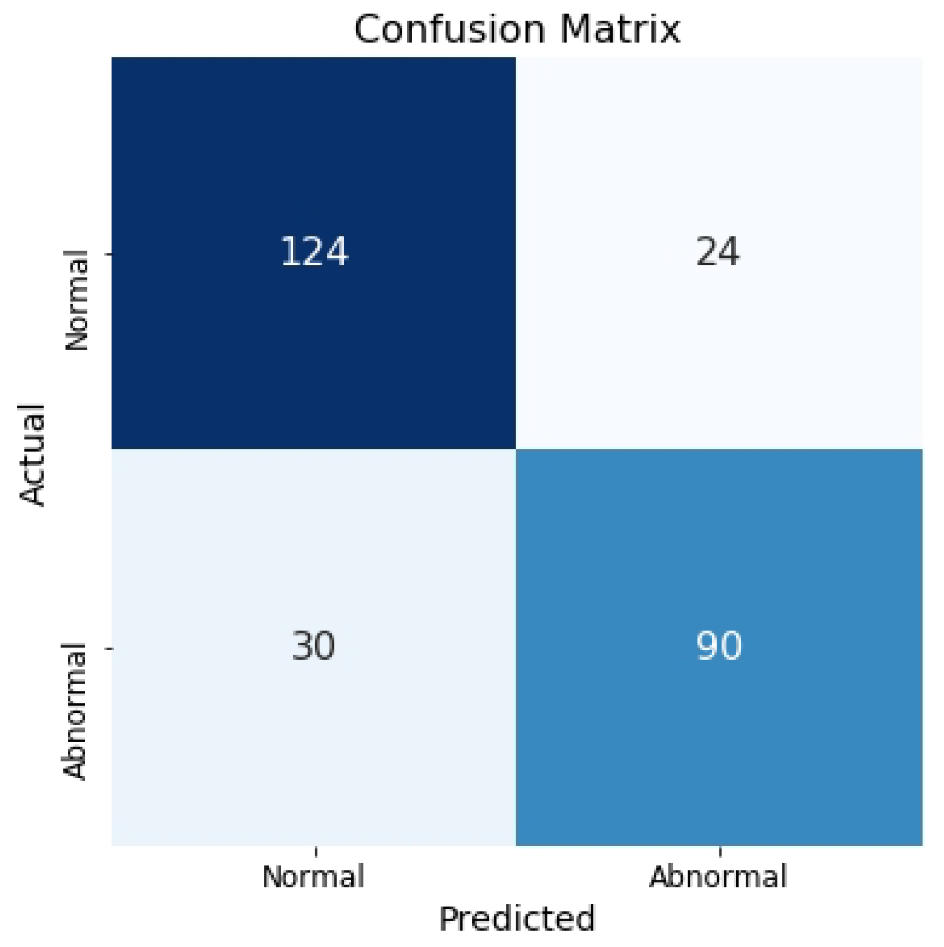Figure 6 presents the confusion matrix for the test set, where spectrograms are used as the input.

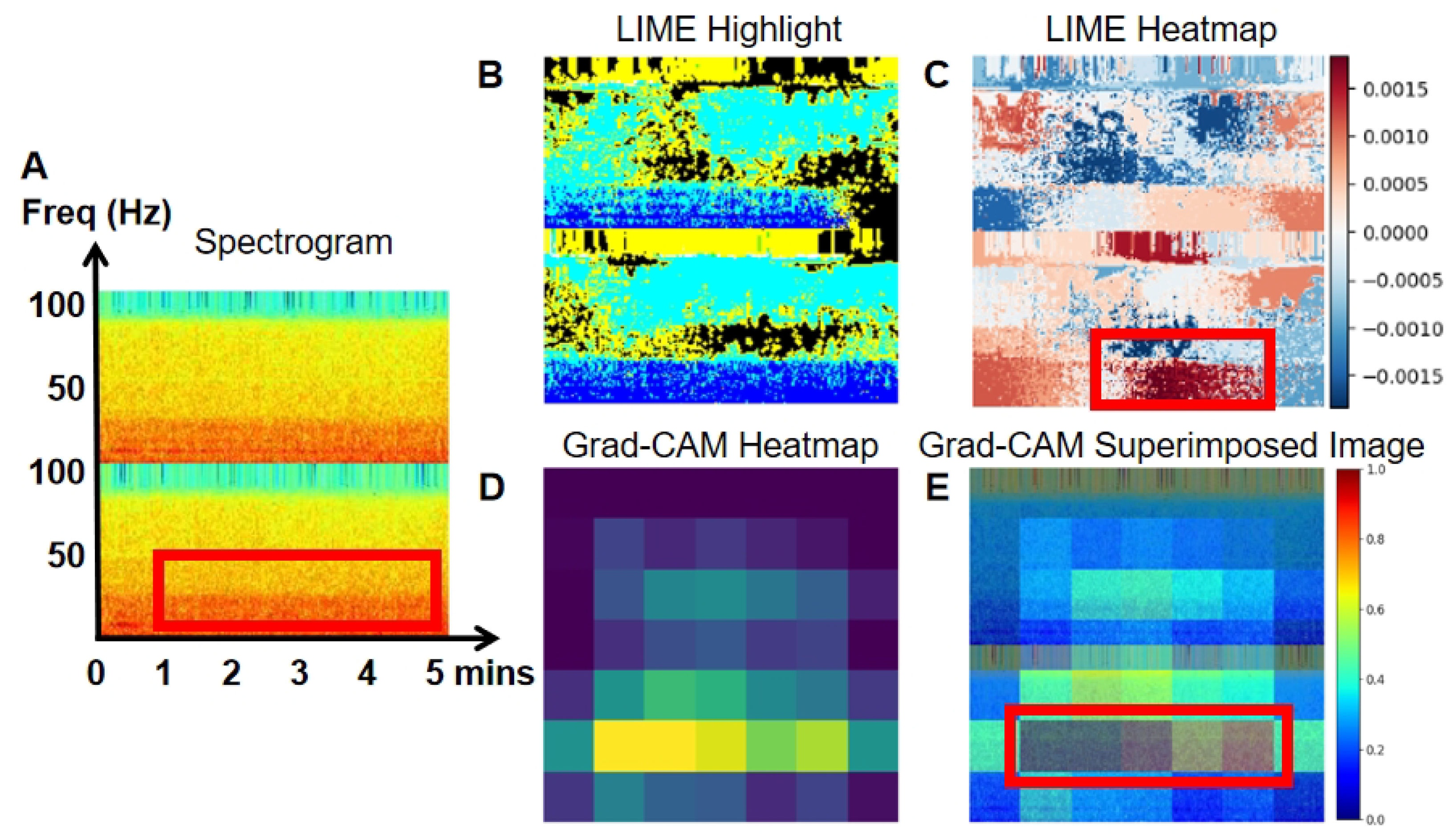
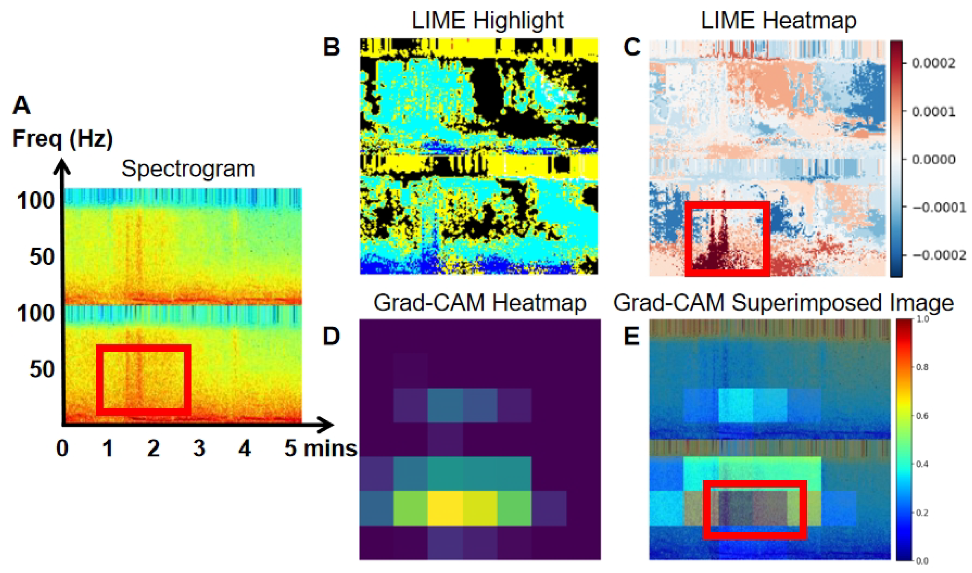
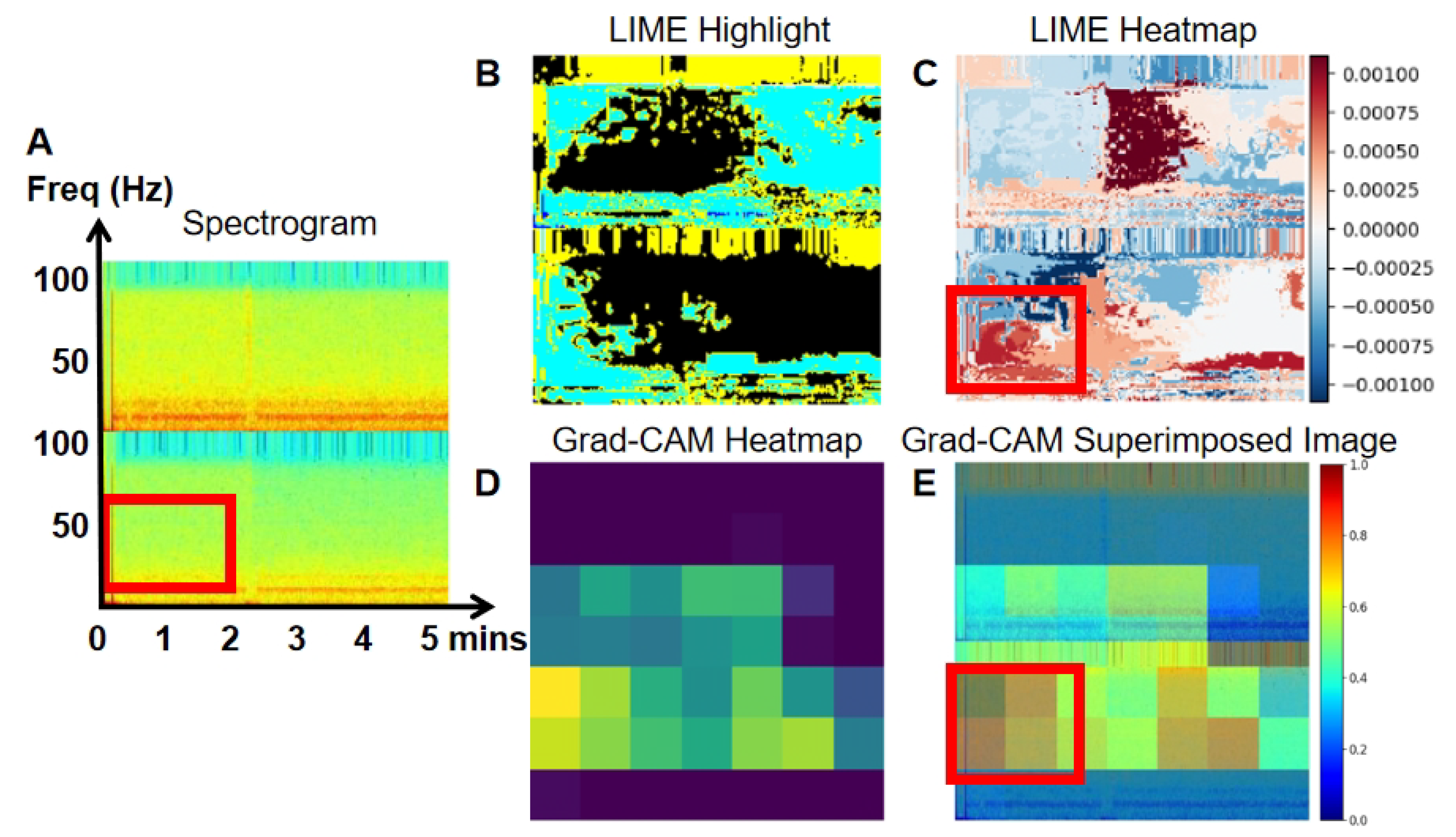
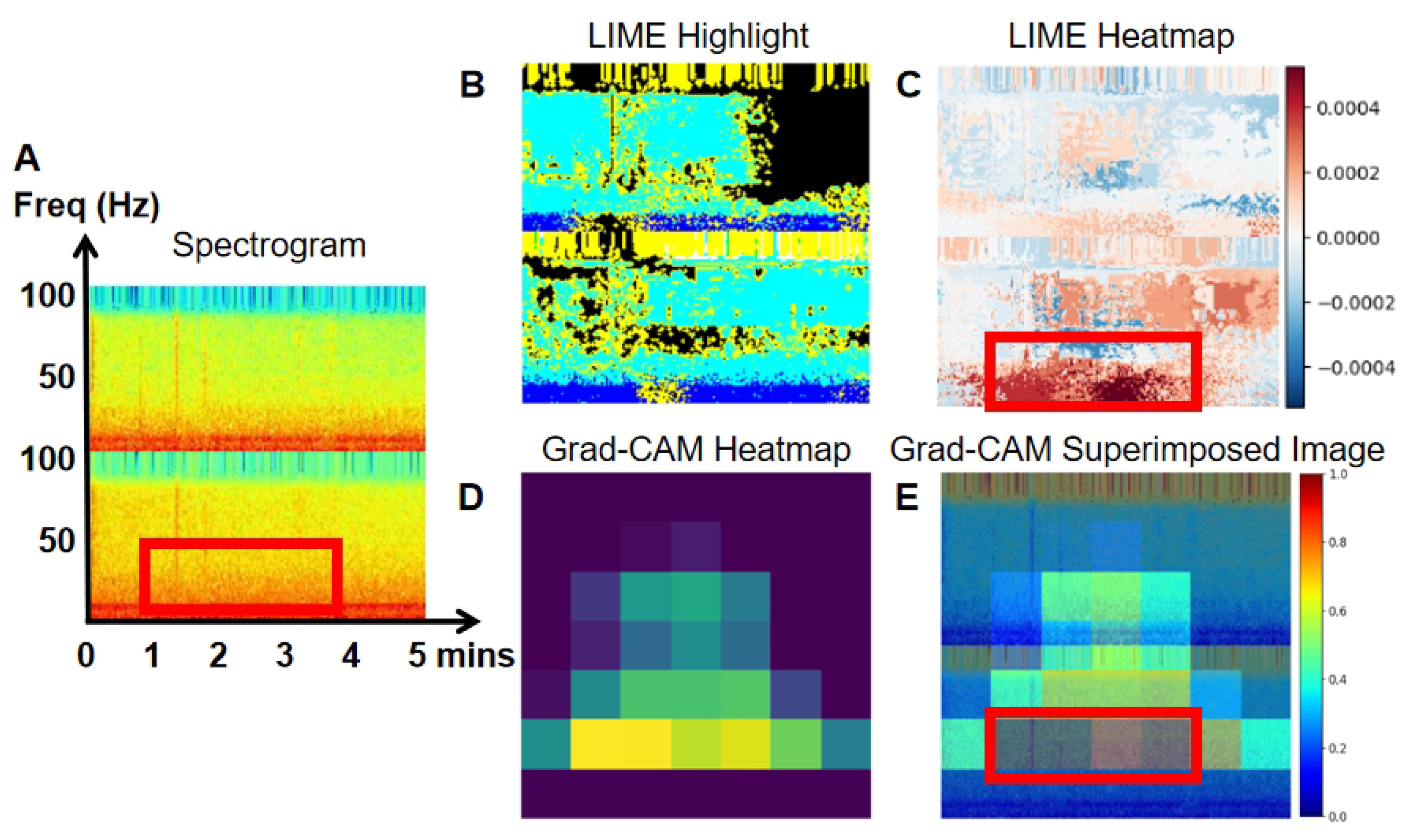
To enhance the interpretability of our model, we employed LIME and Grad-CAM techniques. Figure 7, Figure 8, Figure 9 and Figure 10 present the spectrogram (A), LIME highlights (B), and the heatmap (C) generated by LIME. The spectrogram shows the frequency content of the EEG signal over time, while LIME highlights specific sections of the spectrogram that significantly affect the model’s predictions, aiding in the understanding of classification decisions. The heatmap, generated by LIME, uses color gradients to indicate the importance of different spectrogram regions in the model’s decision-making. Warmer colors (red) represent a positive impact, while cooler colors (blue) indicate a negative impact.

Grad-CAM heatmaps (D) are also shown in Figure 7, Figure 8, Figure 9 and Figure 10. Warmer colors, like red and yellow, highlight regions most influential in the model’s decision, while cooler colors, like blue, represent less significant areas. In the superimposed images, the red and yellow regions align with EEG areas of higher power, frequency, and amplitude, providing deeper insight into the model’s decision-making process in image classification.

Figure 7, Figure 8, Figure 9 and Figure 10 illustrates true positive, true negative, false positive, and false negative events, along with their corresponding LIME (B and C) and Grad-CAM visualizations (D and E), highlighting the specific areas of the spectrogram that the model focused on during classification. In Figure 7, an example of a true positive event is shown. The LIME heatmap (Figure 7C) and Grad-CAM overlay (Figure 7E) clearly highlight the high-power signal with an elevated frequency on channel O1. This signal is marked in blue within the red block on the LIME heatmap, and as the yellow epoch within the red block on the Grad-CAM overlay. The original spectrogram in red indicates higher power at this point. These visualizations demonstrate that this high-power signal plays a crucial role in the model’s prediction of abnormal EEG. The increased power corresponds to the classification of abnormal EEG, as higher power is considered a positive indicator of abnormalities. In contrast, Figure 8 presents a true negative event, where the lower-frequency power signal on channel O1 (within the red block in the Spectrogram, Figure 8A) is crucial for classifying the spectrogram as normal EEG. This comparison highlights that abnormal EEG often shows higher-frequency characteristics compared to normal EEG.

In Figure 9, a false positive event is shown, where elevated power in channels T5 and O1 led to the misclassification of a normal EEG as abnormal. This is highlighted in blue on the LIME heatmap (Figure 9C) and yellow on the Grad-CAM overlay (within the red block, Figure 9E). The misclassification can likely be attributed to artifacts in the spectrogram that misled the model. In contrast, Figure 10, a false negative event, depicts a case where high power at lower frequencies (indicated by the red portion in the spectrogram, Figure 10A) enabled the model to accurately classify the event as normal. However, it is important to note that not all abnormal spectrograms contain detectable abnormal events, resulting in potential misclassifications, particularly false negatives. To address these issues, visualizations produced by LIME (Figure 10C) and Grad-CAM (Figure 10E) can assist researchers in manually correcting such misclassifications. Additionally, we propose a post-processing method in this study aimed at reducing false classification events.

A limitation of the current work is the potential impact of artifacts in the EEG recordings on model performance. While the TUH EEG dataset provides a valuable resource, it may still contain various types of noise and artifacts, such as eye blinks, muscle activity, or electrical interference, which could compromise the quality of the signals. These artifacts, if not properly mitigated, could lead to misclassifications or reduce the overall performance of the model. Although our method includes a post-processing step to average predictions across multiple image outputs, the presence of artifacts in certain segments could still result in false positives or false negatives. Future work should explore more robust artifact removal or detection techniques, such as adaptive filtering or artifact subspace projection, to further enhance the model’s accuracy and reliability in clinical applications.

Another limitation of the current study is that our method was developed and tested only on the TUH EEG dataset. While the results are promising, the model’s performance and generalizability across other EEG datasets or real-world clinical settings remain untested. Variations in data acquisition protocols or patient populations could affect the model’s effectiveness. To enhance robustness and generalizability, future work will involve validating the method on diverse EEG datasets and in real-world clinical environments. This will help assess how well the method generalizes to different populations and recording conditions. Additionally, in future work, we will explore the impact of different EEG channel combinations on model performance, and further analyze the relative importance of each channel in abnormal EEG detection. Moreover, future work would focus on testing the proposed method using more specific datasets to determine its ability to distinguish disease symptoms or differentiate between distinct neurological diseases. For example, datasets related to epilepsy type classification, seizure detection, or seizure prediction could be employed to assess the method’s effectiveness in identifying disease-specific patterns. This will be essential for validating the model’s generalizability and clinical applicability. Furthermore, it is important to note that certain EEG events may be visible in the raw signal but not apparent in the spectrogram or scalogram, potentially affecting model performance [12]. To improve effectiveness and clinical applicability, we plan to integrate raw EEG signals with spectrograms or scalograms in future work, either through input fusion or decision-level ensemble methods.

In addition, to ensure the successful integration of this model into clinical practice, several challenges must be addressed. Real-time deployment in clinical settings requires effective handling of artifacts, rapid processing times, and minimizing false positives and false negatives to avoid clinical misinterpretation. The model’s interpretability is also critical for clinical adoption. Techniques such as LIME and Grad-CAM provide transparency into the model’s decision-making process, which is essential for fostering clinician trust. However, explainability methods may themselves produce inconsistent or overly complex outputs, which could confuse rather than assist clinicians. Therefore, co-designing interpretability outputs with domain experts is crucial. Further validation and refinement of these interpretability tools, in collaboration with clinicians, will be necessary to ensure the model can be integrated into clinical workflows and effectively support decision-making. Additionally, real-world deployment in industrial or embedded systems will require model optimization for resource-constrained hardware, along with rigorous testing to ensure reliability, safety, and compliance with healthcare regulations.

6. Conclusions

In this study, we presented a DenseNet-based method for the classification of entire EEG files as normal or abnormal, focusing on simplifying the process by using fewer channels (T5 and O1). The model demonstrated high accuracy, especially when using spectrogram inputs, and the post-processing method further improved performance by averaging predictions across multiple images. Furthermore, LIME and Grad-CAM techniques were applied to improve the interpretability of the model by visualizing which parts of the input data contributed most to the predictions. These visualizations help explain the model’s decision-making process and allow for a better understanding and potential refinement of the classification method.