Article

Tolerance Proportionality and Computational Stability in Adaptive Parallel-in-Time Runge–Kutta Methods

by
Imre Fekete
1,2,†,
Ferenc Izsák
1,3,*,†,
Vendel P. Kupás
1,† and
Gustaf Söderlind
4,†
1
Department of Applied Analysis and Computational Mathematics, ELTE Eötvös Loránd University, Pázmány P. s. 1/C, 1117 Budapest, Hungary
2
Department of Network and Data Science, Central European University, Quellenstraße 51, 1100 Vienna, Austria
3
NumNet HUN-REN–ELTE Research Group, Eötvös Loránd University, Pázmány P. s. 1/C, 1117 Budapest, Hungary
4
Department of Numerical Analysis, Center for Mathematical Sciences, Lund University, P.O. Box 118, 221 00 Lund, Sweden
*
Author to whom correspondence should be addressed.
These authors contributed equally to this work.
Algorithms 2025, 18(8), 484; https://doi.org/10.3390/a18080484
Submission received: 4 July 2025 / Revised: 30 July 2025 / Accepted: 4 August 2025 / Published: 5 August 2025
(This article belongs to the Section Analysis of Algorithms and Complexity Theory)

Abstract

In this paper, we investigate how adaptive time-integration strategies can be effectively combined with parallel-in-time numerical methods for solving systems of ordinary differential equations. Our focus is particularly on their influence on tolerance proportionality. We examine various grid-refinement strategies within the multigrid reduction-in-time (MGRIT) framework. Our results show that a simple adjustment to the original refinement factor can substantially improve computational stability and reliability. Through numerical experiments on standard test problems using the XBraid library, we demonstrate that parallel-in-time solutions closely match their sequential counterparts. Moreover, with the use of multiple processors, computing time can be significantly reduced.

1. Introduction

Adaptive numerical methods for solving ordinary differential equations (ODEs) have become a significant topic in numerical analysis. The primary motivation for this approach lies in the challenges posed by stiff ODEs, where sudden changes in certain components may occur, and where explicit methods are subject to severe stability restrictions. Such behavior is common, for example, in models of chemical reactions that involve higher-order reaction terms. The steep gradients necessitate very fine time-stepping, which can substantially slow down the simulation.
It is important to note that realistic chemical reaction systems often involve a large number of reaction steps with widely varying reaction-rate coefficients [1]. Similarly, the semi-discretization of large-scale air pollution models [2] can result in ODE systems with a vast number of unknowns.
To address this, it is essential to identify regions where steep gradients occur, applying small time steps in their vicinity. Several algorithms have been proposed in the literature to construct efficient adaptive refinements (see [3], Section 5.2).
We begin by noting that any spatial semi-discretization of partial differential equations (PDEs) yields a large, stiff system of ordinary differential equations (ODEs). As a result, efficient numerical methods are required—even when the reaction terms are nonstiff.
However, heuristic algorithms for selecting time steps can be prone to instabilities. For instance, it is important to adjust the time steps smoothly by controlling the ratio between successive step sizes. This necessity naturally connects time-step selection with control theory. Indeed, some of the most effective adaptive time-stepping algorithms have been developed using control-theoretic approaches. Further details can be found in the classical works [4,5,6,7]. For a recent approach, we refer readers to [8].
Another strategy for accelerating the numerical solution of ODEs is to use parallel-in-time algorithms. Over the past decade, interest in these methods has been revitalized by the advent of massively parallel computing architectures. In addition to traditional applications involving PDEs [9,10,11,12], recent developments such as neural ordinary differential equations [13] and physics-informed neural networks [14] have further broadened the scope of parallel-in-time methods, especially in machine learning and deep learning contexts [15,16,17,18].
Parallel-in-time methods can be broadly categorized into four main groups: multiple shooting methods; domain decomposition and waveform relaxation methods; space-time multigrid methods; and direct parallel-in-time algorithms. A comprehensive overview of these techniques is provided in the review paper [19] and the monograph [20].
In this work, we focus on the multigrid reduction-in-time (MGRIT) method introduced in [21]. MGRIT is closely related to the parareal algorithm developed in [22] and has since been extended in a variety of directions. These include applications to nonlinear parabolic equations [23], adaptive (variable-step) multistep methods [24], layer-parallel training of deep residual neural networks [25], efficiency improvements via Richardson extrapolation [26], and hyperbolic problems such as linear advection [27].
Adaptive parallel-in-time methods have been explored in [24,26], with a primary focus on metrics such as time versus discretization error and processor versus wall-clock time. However, another important aspect of reliability is how the global error responds to changes in the specified tolerance. Ideally, for problems with regular solutions, a small change in the tolerance should result in a proportionally small change in the error. This property, referred to as tolerance proportionality, is fundamental to computational stability [28].
In Section 2, we introduce the necessary concepts and tools—such as the MGRIT algorithm, basic sequential adaptive strategies, tolerance proportionality, and computational stability—that motivate the modified refinement factor presented in the subsequent section. In Section 3, as the main novelty of the paper, we demonstrate both tolerance proportionality and computational stability in our advanced parallel-in-time method, which builds upon the step-size selection strategy proposed in [24]. The proposed approach is validated through several test problems, including classical ODE systems and systems arising from the discretization of PDEs. All numerical results can be reproduced using the public GitHub repository [29]. Finally, in Section 4, we discuss the advantages, limitations, and corresponding directions for future research.

2. Preliminaries: Main Tools and Requirements

In this section, we introduce the fundamental components of our algorithm and outline the key practical requirements it must fulfill.

2.1. The MGRIT Algorithm

We provide a brief overview of the MGRIT method introduced in [21]. Assume we are given the initial value problem
u ( t ) = f ( t , u ( t ) ) , t ( 0 , T ) , u ( 0 ) = u 0 ,
where f is a given function and u 0 is the initial condition. Let 0 = t 0 < t 1 < < t N 1 < t N = T be a uniform mesh given on the interval [ 0 , T ] with an equidistant step size Δ t .
In standard time-stepping approaches, the solution is approximated using a one-step method
u 0 = u 0 , u i + 1 = Φ i + 1 ( u i ) + g i + 1 , i = 0 , 1 , , N 1 ,
where Φ denotes the one-step update operator, which can be practically any Runge–Kutta method, and g represents the source or correction terms. Since each time point depends on the previous one, this yields a sequential algorithm in time.
In contrast, the MGRIT algorithm iteratively computes an approximation to the solution over the entire time domain, starting from an initial guess. MGRIT is based on multigrid techniques and enables parallelization in the temporal domain. Assume that the right-hand side f is linear, and consider a coarser time grid 0 = T 0 < T 1 < < T N m 1 < T N m = T with a step size Δ T = m Δ t . On this coarse grid, we apply another one-step method, denoted by Φ Δ , which is computationally cheap and used to improve the current approximation. The two-grid method, which is equivalent to the parareal method [22], is outlined in Algorithm 1. The relaxation steps are illustrated in Figure 1.
Algorithm 1 Two-grid method.
1:
Relaxation by F-relaxation (or FCF-relaxation)
2:
Restriction: r Δ , i = u m i ( Φ m i ( u m i 1 ) g m i )
3:
Solve the problem v Δ , i = Φ Δ ( v Δ , i 1 ) + r Δ , i in the coarse grid
4:
Prolongation: u i m = u i m + v Δ , i
5:
Relaxation by F-relaxation
The convergence rate of the two-grid method depends on how accurately the coarse-grid propagator Φ Δ approximates the result of performing m successive fine-grid steps between two coarse time points. Selecting an optimal coarse-grid propagator remains an active area of research. In many practical settings, the same numerical method is employed on both the fine and coarse grids.
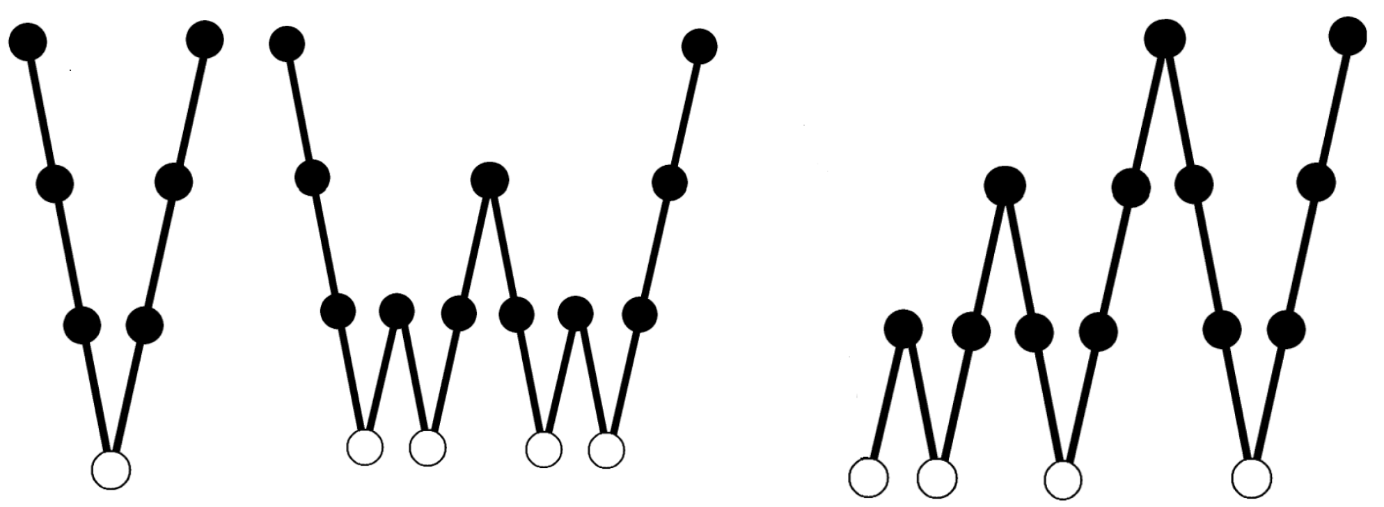
A potential limitation of the two-grid approach is that the coarse grid may still be too fine, rendering Step 3 of Algorithm 1 computationally expensive. This issue can be addressed by recursively applying the same algorithm on increasingly coarser grids, following the classical multigrid paradigm. The resulting recursive structure gives rise to various cycle types, such as V-, W-, and F-cycles, as illustrated in Figure 2. Furthermore, the algorithm can be extended to nonlinear problems using the Full Approximation Scheme (FAS).
The MGRIT algorithm achieves optimal complexity with a runtime of O ( N ) and, unlike traditional time-stepping schemes, is massively parallelizable. In practice, convergence to a sufficiently accurate solution is often attained within a few iterations. The numerical results of strong scaling studies on a linear problem (heat equation) and a nonlinear problem (p-Laplace problem) are presented in [21,23]. These results show that while the sequential one-step method outperforms MGRIT with a small number of processors, significant speedup is achieved when parallel resources are effectively utilized.
The XBraid software package is an implementation of the MGRIT method [30]. It is written in MPI/C with interfaces for C++, Fortran 90, and Python, and is designed to be non-intrusive. This allows users to leverage their existing sequential time-stepping code, while XBraid manages the parallelization. Additionally, XBraid supports time refinement, enabling adaptive time-stepping strategies within the parallel-in-time framework. We used this implementation of the MGRIT method in the experiments presented in the next section.

2.2. Tolerance Proportionality and Computational Stability

If a method and its step size have been chosen properly for a given problem, it typically operates in the asymptotic regime. Thus, if the method order is p, the norm of the local error at time t n is well approximated by
l n = ψ ( t n ) h n p ,
where h n is the current step size and ψ ( t ) is the principal error function. The latter is smooth provided that the regularity of the solution is sufficiently high. When the regularity is low, it is often preferable to use a low-order method, i.e., reduce p to match the regularity of the solution so that we again have a local error of the form (1) with a smooth function ψ ( · ) . In adaptive step-size selection based on local error control, the objective is to keep the local error constant, equal to a prescribed tolerance TOL , i.e.,
l n = ψ ( t n ) h n p = TOL h n = TOL ψ ( t n ) 1 / p .
It follows that the “proper” step-size sequence is smooth, and that
log h n = 1 p log TOL log ψ ( t n ) .
Hence, if the logarithm of the step-size sequence { log h } is plotted vs. time, a change in TOL merely shifts the graph given by { log ψ } vertically. In other words, the proper step-size sequence is a smooth function negatively correlated with the principal error function, with { log h } proportional to log TOL .
For these reasons, any step-size selection scheme should aim to replicate these properties. Thus, the generated step-size sequence should be smooth, and if well implemented, the tolerance proportionality should be readily visible in real computations. If the global error accumulation is regular, this implies that the global error should be proportional to the tolerance. This can, however, only be achieved with careful implementation (see, e.g., [28]). In practice, tolerance proportionality means that the global error u i u ( t i ) is bounded below and above by the expression
c · TOL u i u ( t i ) C · TOL ,
where the two constants satisfy c / C 1 . Note that this is a fairly rigorous requirement; we not only require that the local error is less than TOL but also that it is near TOL . Thus, if TOL is increased or reduced by a small factor, the error must change accordingly, increasing or decreasing in proportion. This is also referred to as computational stability, as the computational algorithm is required to produce accurate approximations in the sense that the error stays near that of previous results. In the present context, we aim to investigate whether it is also possible to retain such properties in parallel integration.

2.3. Classical Recursive Controllers

In sequential computing, the conventional step-size selection scheme is of the form h n + 1 = ρ n · h n , i.e., the step-size sequence is generated recursively along the solution trajectory. Taking logarithms, we obtain a linear recursion,
log h n + 1 = log h n + log ρ n ,
i.e., we have a simple summation process, referred to as an integral (or I) control. The quantity being summed is the control error log ρ n . In the simplest case, one takes
ρ n = e n TOL 1 / p ,
where e n is the local error estimate. This changes (2) into
log h n + 1 = log h n + 1 p log e n log TOL ,
where the deviation log e n log TOL is the control error. The step size keeps changing unless the control error is zero. Note that, in order to generate a smooth step-size sequence, we basically advocate changing the step size every step, no matter how small the change is. Thus, older schemes of step-size halving/doubling typically generate nonsmooth step-size sequences, although it may not be possible to avoid such sequences in connection with multigrid-type step-size refinement.
There are many more advanced alternatives to the elementary controller (3). Some more general recursive controllers have the form
h n + 1 = ρ n β 0 ρ n 1 β 1 ρ n 2 β 2 · h n ,
where the ρ i is given by (3) and the coefficients β 0 , β 1 , β 2 can be chosen to improve both stability and regularity, notably by using techniques from digital filtering (see [6,7]). Depending on the resulting structure, the controllers may be referred to as proportional–integral (PI control) or proportional–integral–derivative (PID) control. An important aspect is being able to reduce the gain of the controller, as the elementary controller (3) is sometimes prone to generating oscillatory (nonsmooth) step-size sequences. There are also further possibilities that account for previous step-size sequences. The design of the controller should be matched to the type of method and the problem class. Thus, stiff integration can benefit from special implicit methods with dedicated time-step adaptivity.
In the present context, experiments are based on variants of (3) due to the special requirements associated with multigrid refinement.

3. Results

The adaptivity strategy described in [24] starts with an equidistant coarse time grid, which is further refined where necessary based on the error estimator during a given step. The refinement factor r is computed as the ratio of the current step size to the one suggested by the error estimator. Assuming that the step size–error relation is in the asymptotic regime, the refinement factor is constructed from the formula
r = h n h n + 1 = e n TOL 1 / p ,
where e n is the error estimate, TOL is the user-provided accuracy requirement, and p is the order of the error estimator of the Runge–Kutta method. The ceiling function is motivated by the fact that the subintervals can only be divided into an integer number of smaller subintervals. A schematic concept of the refinement factor r is shown in Figure 3.
The formula (5) without the ceiling function resembles the classical elementary I–controller (3) (cf. [4], Chapter II.4). Therefore, we would expect tolerance proportionality properties similar to those in sequential integration, reducing the losses at the interfaces of intervals with different refinement factors. The importance of smooth step-size sequences lies in the fact that the local errors can be equidistributed, a principle that is usually conducive to uniform global error behavior as a function of TOL .

3.1. ODE Test Problems

The first test problem is the two-compartment dilution process:
y 1 = 1 5 y 1 y 2 = 2 5 ( y 2 y 1 )
for t [ 0 , 20 ] , with the exact solution
y 1 = 0.3 e 0.2 t y 2 = 0.6 ( e 0.2 t e 0.4 t ) .
The initial values were chosen as the exact solution values at the first step. This linear problem is a standard test case with a known solution, making it ideal for assessing time-discretization accuracy and efficiency.
The second test problem is the classical nonlinear Lotka–Volterra equation:
y 1 = 0.1 y 1 0.3 y 1 y 2 y 2 = 0.5 ( y 1 1 ) y 2
for t [ 0 , 62 ] . The initial values were taken as [ 1 , 1 ] .
The third problem is the classical van der Pol equation:
y 1 = y 2 y 2 = μ ( 1 y 1 2 ) y 2 y 1
with t [ 0 , 20 ] . The initial values were [ 2 , 0 ] . This is also a classical nonlinear test problem because it transitions from nonstiff to stiff behavior as the parameter μ increases. We chose μ = 2 for the nonstiff computation.

3.2. Results for Refinement Factors r, r m o d , and r exp

For the ODE test problems in Section 3.1, smooth step-size sequences produced tolerance proportionality in the sequential case. The MGRIT procedure, together with (5) from the open-source XBraid library [30], was used with the Bogacki–Shampine method to take into account its stability region.
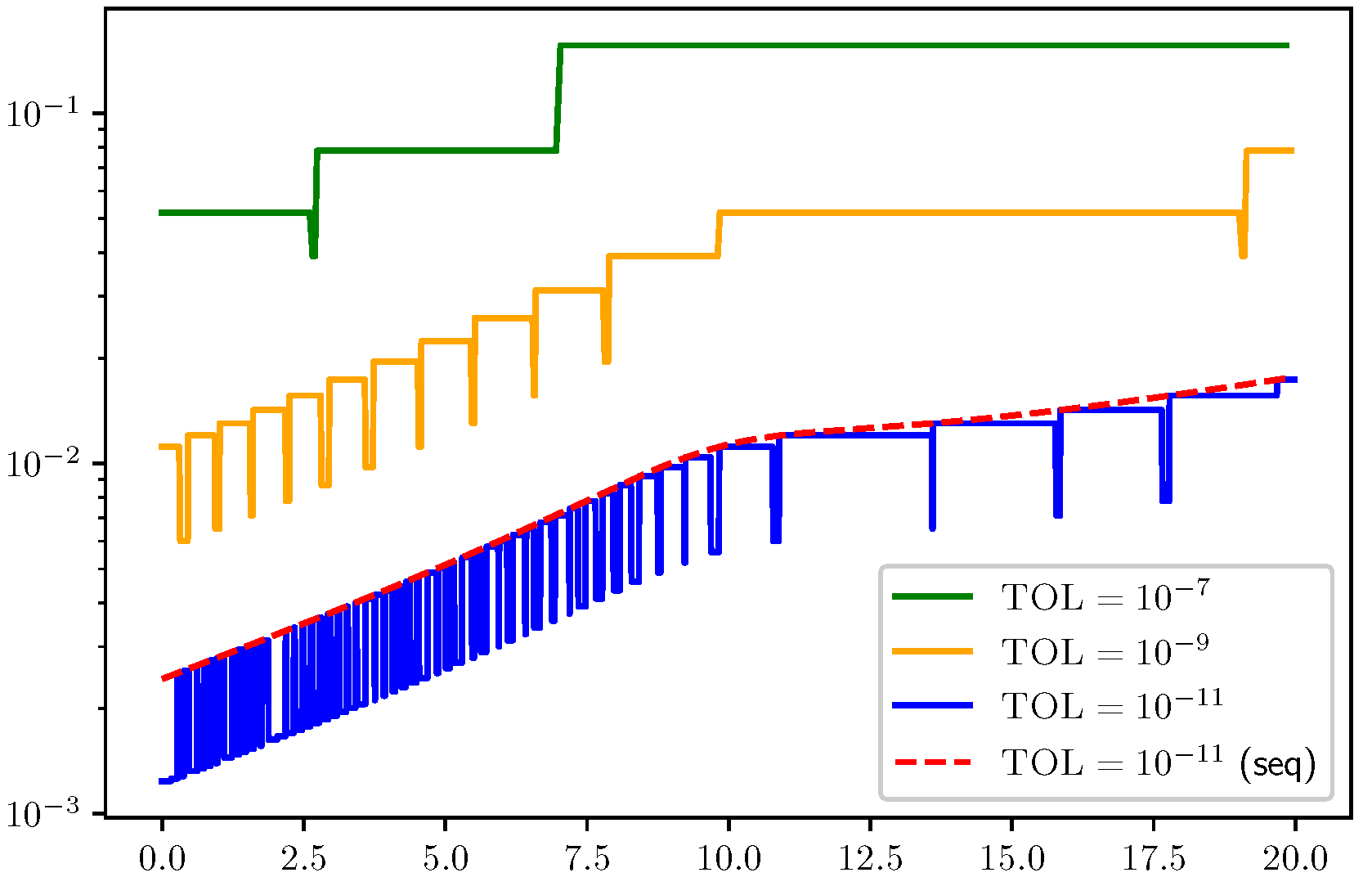
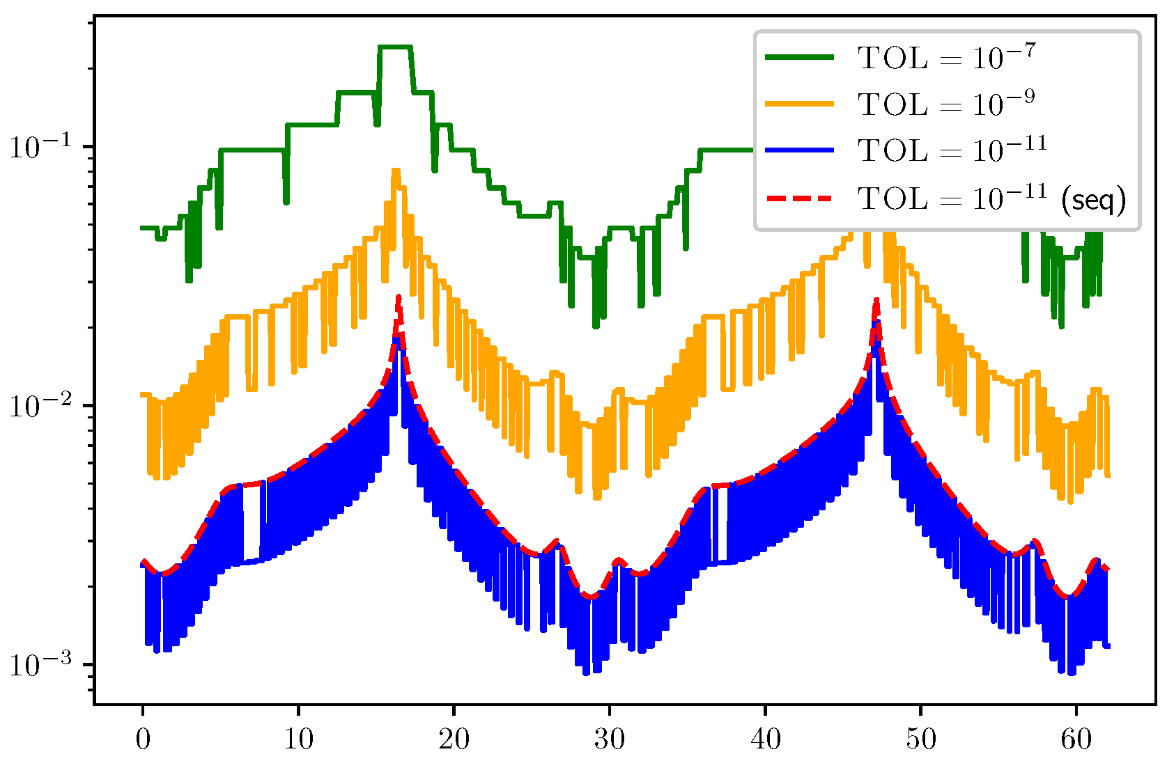
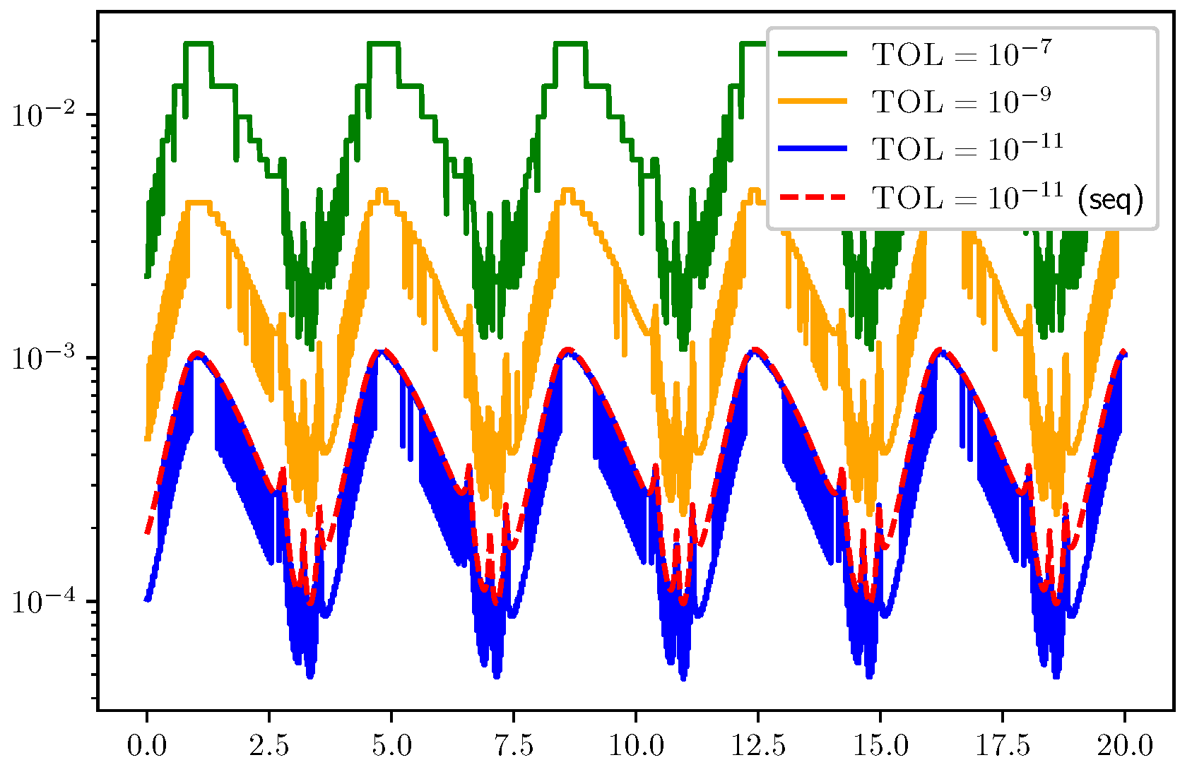
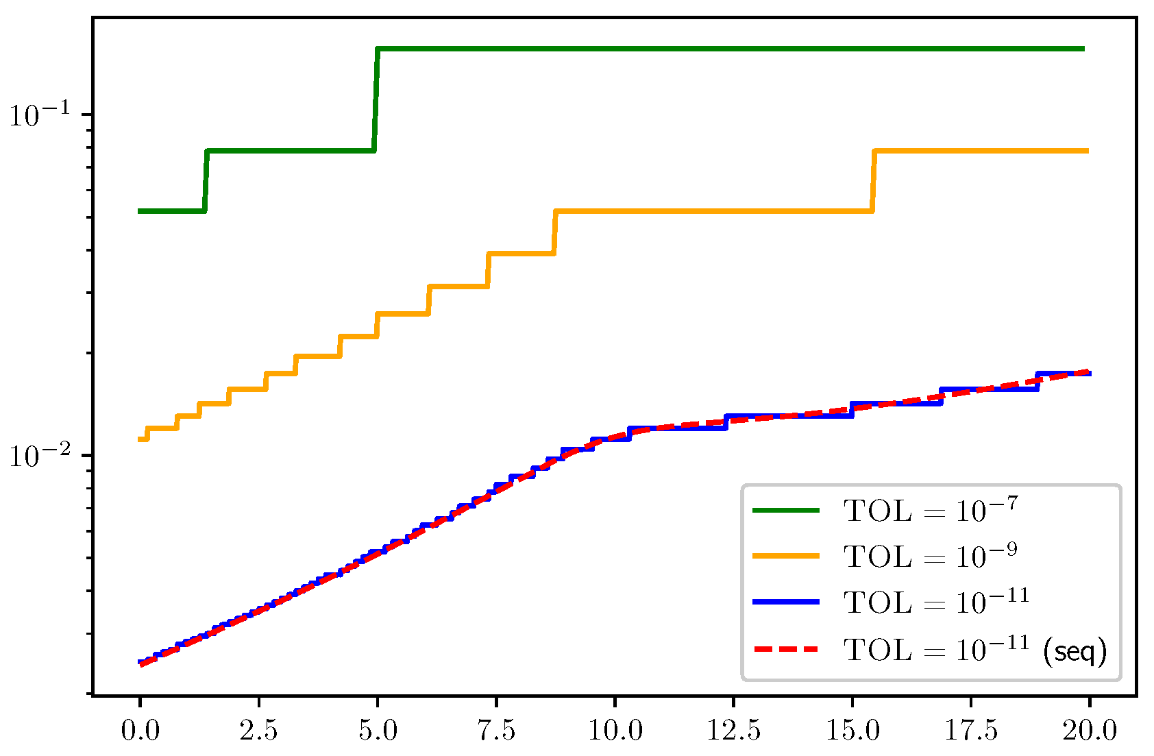
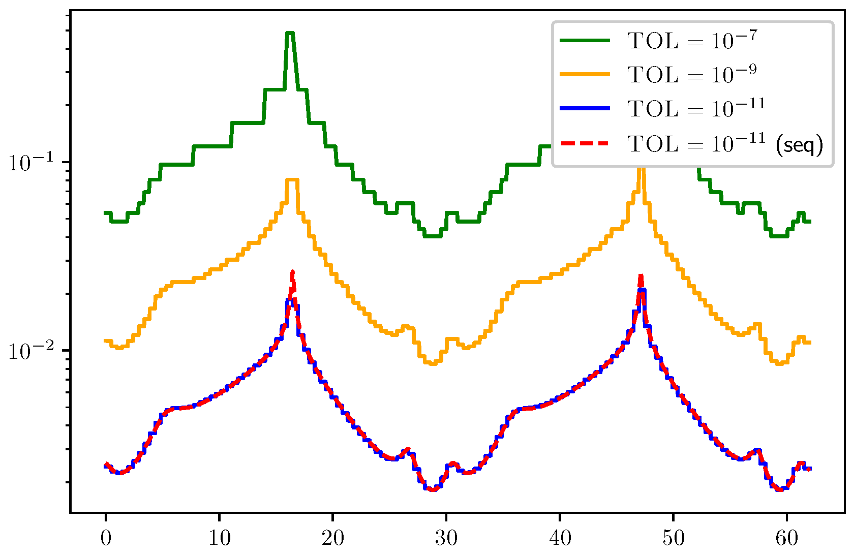
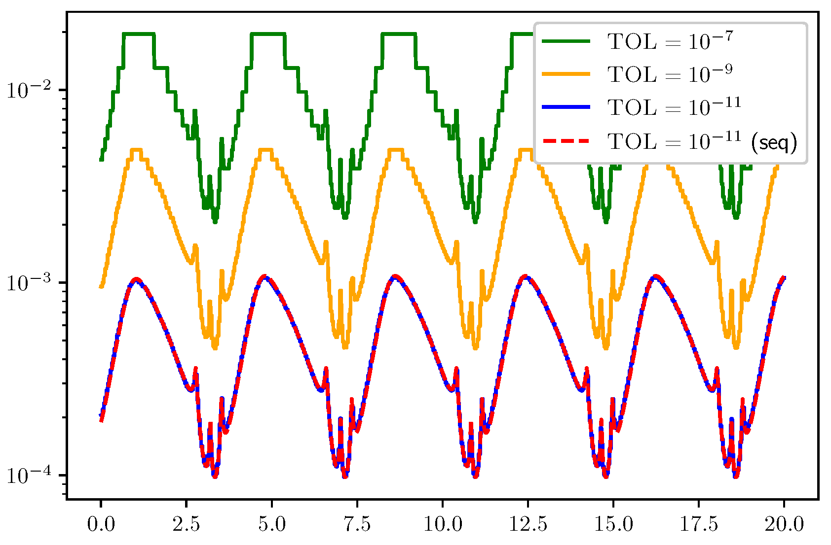
The tolerance proportionality results can be seen in Figure 4, Figure 5 and Figure 6. In Figure 4, Figure 5 and Figure 6, we plot the step-size sequence for each test problem. A reasonable error tolerance proportionality is observed, as the step size on average scales in accordance with the specified error tolerance. At the finest tolerance, TOL = 10 11 , the MGRIT-based step-size sequence is also close to that of the sequential integration for the same tolerance.
However, in every test case, a zigzag pattern appears in the step-size sequence, which contrasts with the smooth step-size sequence expected in classical sequential implementation theory [7]. This effect arises since the refinement factor is highly sensitive to small values due to the ceiling function. Pointwise tolerance proportionality therefore suffers, and it is unlikely that the overall method is as efficient as it could be, since local errors are far from equidistributed.
We therefore conclude that it is worth considering alternatives to (5). Thus, we define a modified refinement factor r m o d as follows:
r m o d = h n h n + 1 = e n TOL 1 / p c .
Here, the compensating constant is taken as c [ 0.2 , 0.4 ] in (9).

3.2.1. The Final Algorithm with r mod

Completing the adaptive MGRIT procedure with this essential modification and summarizing all steps, we apply the following algorithm:
(A1)
Set an initial temporal grid and an initial guess of the solution (see Figure 3).
(A2)
Apply a given Runge–Kutta method in parallel from these initial values, and use multigrid cycles to improve the current approximation of the solution (see Figure 2).
(A3)
Determine the refinement factor for each subinterval on the finest grid based on (9).
(A4)
IF no refinement occurred and the accuracy criterion is satisfied then STOP.
(A5)
ELSE go to Step 2.
For the tests, we used the embedded Runge–Kutta methods (described later) for time stepping and error estimation. We started on a uniform temporal grid and applied three V-cycles between two consecutive refinements. As shown in Figure 7, Figure 8 and Figure 9, the modified refinement largely suppressed the zigzag patterns, resulting in smoother step-size sequences and improved tolerance proportionality.

3.2.2. An Attempt with Exponential-Forgetting Filters

An alternative idea is to reduce the integral gain in (5) from 1 to, say, 2 / 3 , i.e., change the exponent from 1 / p to 2 / ( 3 p ) by constructing another modified refinement factor. As this corresponds to an exponential-forgetting filter, we denote this new refinement factor by r exp . However, this does not result in a smoother step-size sequence, although it is well known to have such an effect in the sequential case. Again, this appears to be due to the ceiling function. The corresponding figures can be found in the GitHub repository [29].

3.2.3. Tolerance Proportionality for the Algorithm (A1)–(A5)

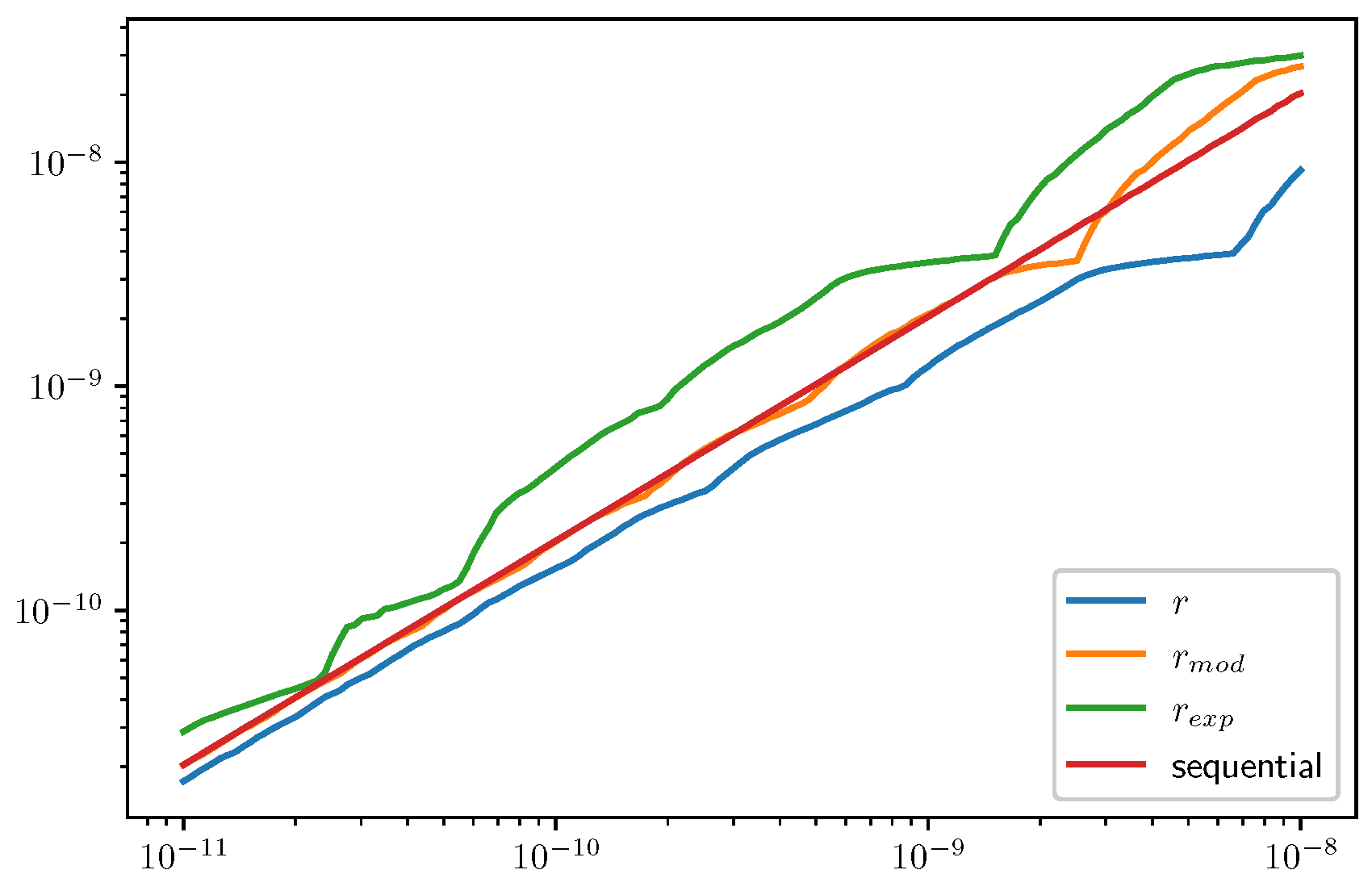
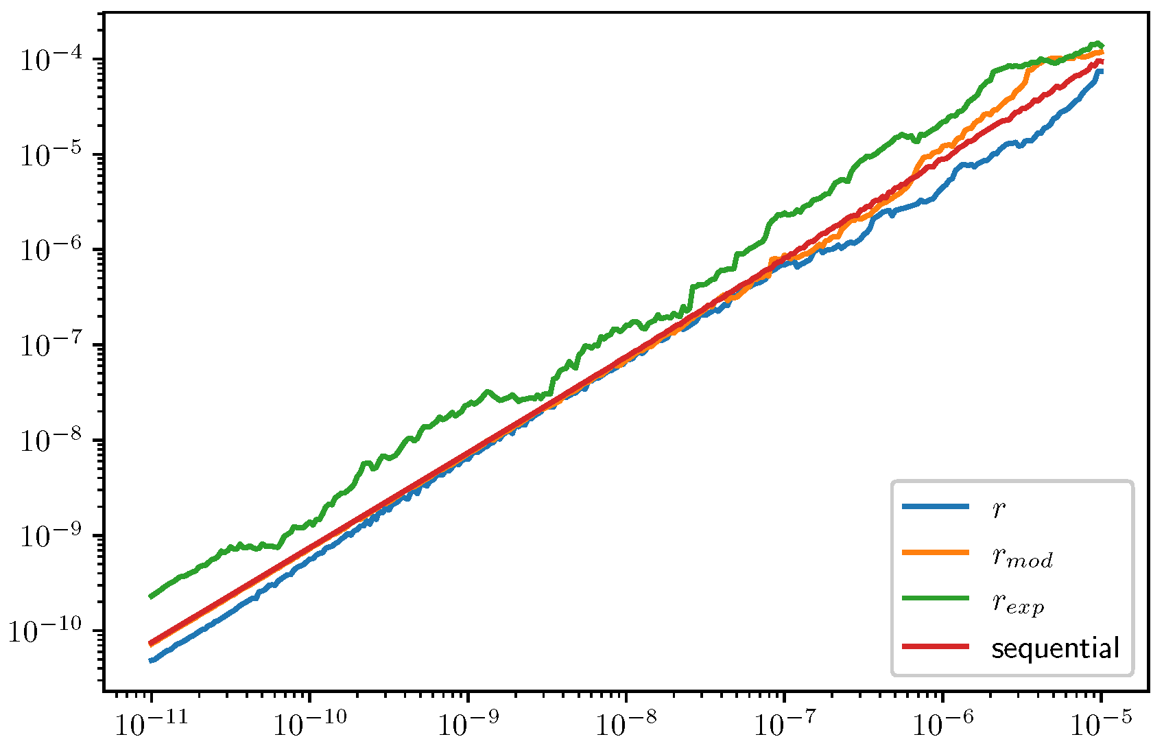
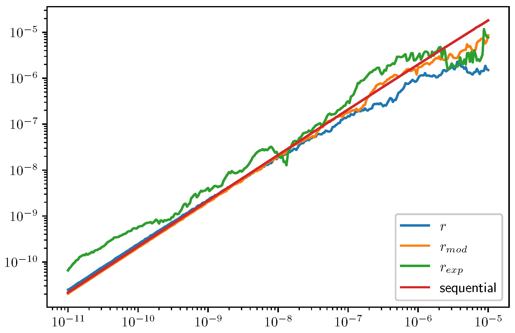
In connection with the concept of computational stability discussed in [28], the achieved accuracy is plotted versus TOL . Ideally, a log–log plot would be expected to show a nearly straight line if the step-size sequence accurately tracks the local errors. This tolerance proportionality ensures that a reduction in TOL leads to a corresponding improvement in the achieved accuracy. This accuracy versus tolerance for the three different approaches is shown in Figure 10, Figure 11 and Figure 12.
Based on Figure 10, Figure 11 and Figure 12, the refinement factor r m o d demonstrates the best computational stability while maintaining performance comparable to sequential computation. For sharp tolerances, the results are effectively identical. In contrast, the exponential-forgetting alternative r exp provides less benefit.
Based on Figure 4, Figure 5, Figure 6, Figure 7, Figure 8, Figure 9, Figure 10, Figure 11 and Figure 12, it is qualitatively clear that r m o d is the best among the three discussed refinement factors. Naturally, one may ask whether the suppression of zigzag patterns is also beneficial in a quantitative sense. To investigate this, we compare the r m o d refinement factor with the less zigzag-prone r refinement factor rather than with the more erratic r exp . As shown in Table 1, r m o d makes the step-size sequences smoother, improves tolerance proportionality, and significantly reduces computational cost.

3.3. PDE Test Problems and Related Results

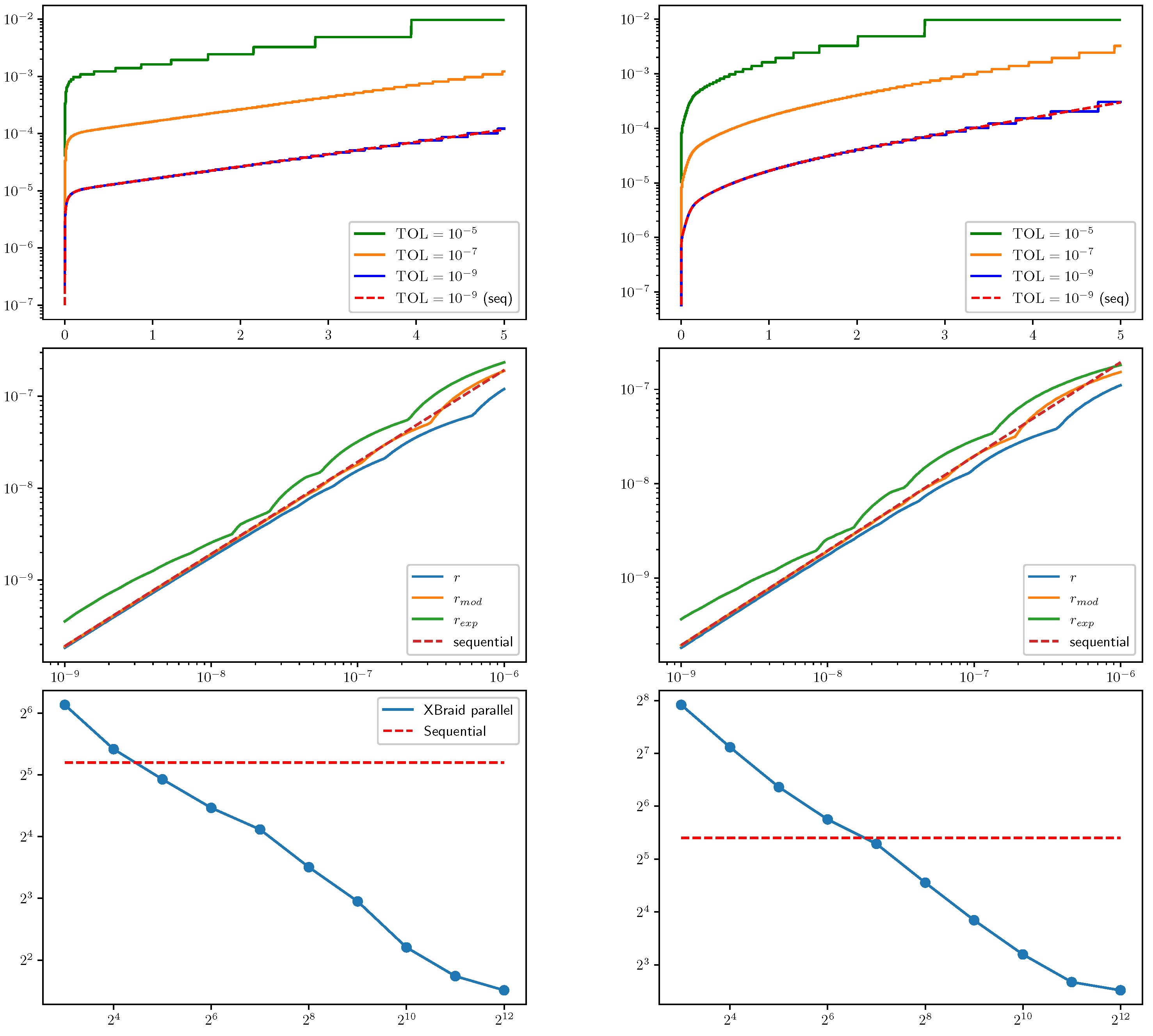
For the three ODE test problems in Section 3.1, there was no significant difference in runtime between the sequential and MGRIT-based parallel-in-time algorithms using eight processors. However, a notable runtime advantage was observed in the case of partial differential equations (PDEs).
Our test problems for PDEs are special cases of one-dimensional, possibly nonlinear diffusion equations with Dirichlet boundary conditions. Specifically, we consider the following formulation:
t u ( t , x ) = 1 10 x x ( u p ( t , x ) ) , x ( 0 , 1 ) , t ( 0 , 5 ) u ( 0 , x ) = g ( x ) , x ( 0 , 1 ) u ( t , 0 ) = g ( 0 ) and u ( t , 1 ) = g ( 1 ) , t [ 0 , 5 ] ,
where g ( x ) = 10 e ( x 0.435576 ) 2 7.27185 . The linear case corresponds to p = 1 , while we take p = 2 in the nonlinear case. Based on the ODE test results in Section 3.2, we only consider the modified refinement factor r m o d using c = 0.4 . In space, we use the classical second-order central difference scheme. For time integration, we use a two-stage, stiffly accurate, L-stable, singly diagonally implicit Runge–Kutta method (see [31], Butcher tableau (221), with the choices γ = ( 2 2 ) / 2 and b ^ 2 = 0 ). When selecting the spatial and temporal step sizes, we make sure that the necessary CFL condition is satisfied, both for p = 1 and p = 2 in (10). The results related to the tolerance proportionality, achieved accuracy, and runtime can be seen in Figure 13.
Figure 13 demonstrates that both the linear and nonlinear diffusion Equation (10) show good tolerance proportionality and computational stability, as well as the expected qualitative behavior of achieved accuracy versus tolerance. In addition, the expected reduction in runtime due to parallelization is also observed.

4. Discussion

We summarize the main advantages of our proposed method and, for the sake of completeness, also highlight the limitations of the framework, which suggest interesting research directions in their own right.

4.1. Advantages

The computational results in Section 3 indicate that for MGRIT-based adaptive parallel-in-time Runge–Kutta methods, the relevant quality indicators necessary for computational stability are satisfied for the refinement factors r m o d and r. As we have seen in the case of the PDE test problems in Section 3.3, these methods significantly outperform sequential methods in terms of computational cost beyond a certain number of processors. Furthermore, based on the qualitative results of the different ODE and PDE test problems, as well as the number of time steps in Table 1, the refinement factor r m o d is the preferred approach both qualitatively and quantitatively. Therefore, the approach involving the refinement factor r m o d provides a robust and reliable framework for users utilizing high-performance computing simulations.

4.2. Limitations

The first limitation is that, for each test problem, the MGRIT algorithm must be run with an appropriate initial subinterval partitioning to achieve computational stability. Figure 14 illustrates this phenomenon. This characteristic can be seen as analogous to the choice of the initial step size in sequential algorithms (see [4], Chapter II.4, and [32], Section 4.2).
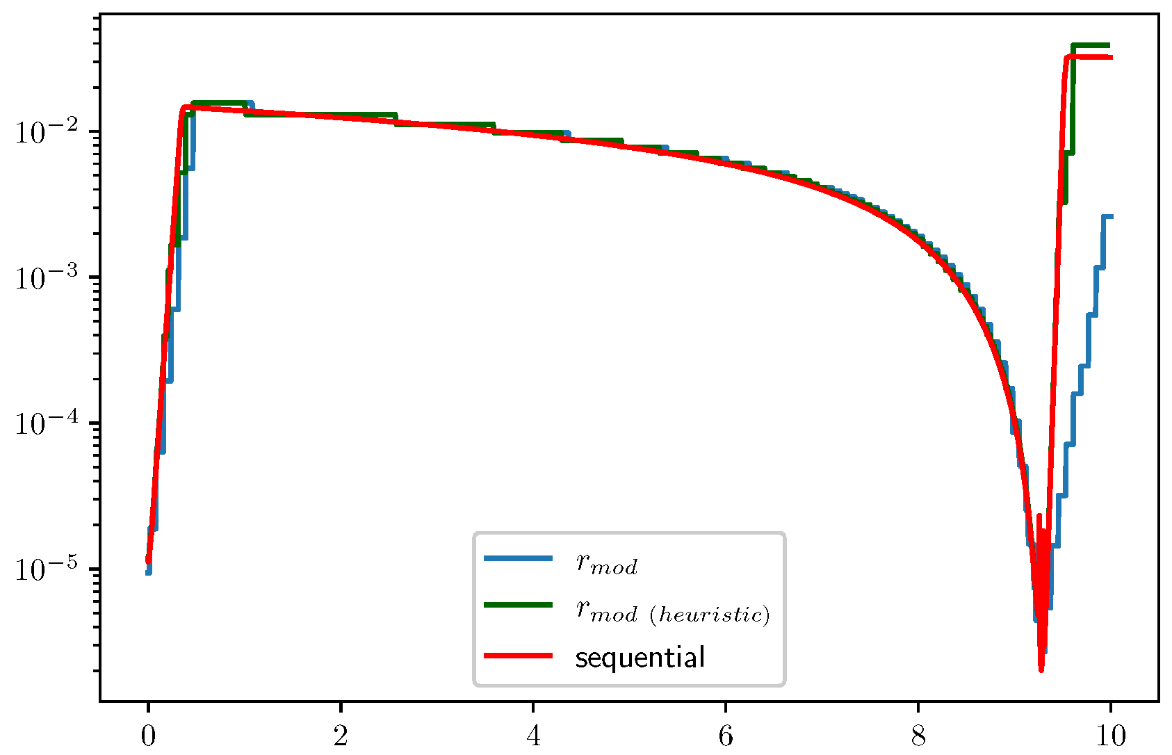
The second limitation may be that our current results have provided satisfactory quality only for nonstiff (or at most mildly stiff) problems. This naturally suggests a research direction focusing on stiff problems. Due to their much larger variation in step sizes, they pose a more significant challenge. Based on the structure of MGRIT methods, it is clear that the analogy of PI- and PID-type controllers (4), which are commonly used in sequential algorithms (for details, see [7]), needs reconsideration in this setting. However, from this theoretical background, we also know that for stiff problems, PI controllers of a different parametrization are needed. An example of this can be seen in Figure 15, which illustrates the case of the stiff van der Pol equation (8) with μ = 30 and initial value [ 1.5 , 3 ] on the time interval [ 0 , 10 ] . Using heuristics, we were able to significantly improve the step-size sequence.

4.3. Future Research

A closer examination of the above-mentioned heuristic is needed to fully understand its role in connection with parallel-in-time methods. Based on our observations, we also conclude that by incorporating a stiffness indicator (for details, see [33] and [34], Chapter 21.3) as a measuring and switching mechanism, we may obtain better results for stiff problems in the current framework. Further research in this direction will lead to dedicated methods specifically designed for stiff problems.
All simulation figures (Figure 4, Figure 5, Figure 6, Figure 7, Figure 8, Figure 9, Figure 10, Figure 11, Figure 12, Figure 13, Figure 14 and Figure 15) in this work are fully reproducible using the files available in the GitHub repository [29].

Author Contributions

Conceptualization, I.F. and G.S.; methodology, I.F.; software, V.P.K.; validation, V.P.K. and I.F.; formal analysis, F.I. and G.S.; investigation, F.I.; resources, I.F.; data curation, I.F. and V.P.K.; writing—original draft preparation, F.I.; writing—review and editing, F.I., I.F., and G.S.; visualization, V.P.K.; supervision, I.F. and F.I.; project administration, I.F.; funding acquisition, I.F. All authors have read and agreed to the published version of the manuscript.

Funding

This research was supported by the Ministry of Innovation and Technology NRDI Office within the framework of the Artificial Intelligence National Laboratory Program RRF-2.3.1-21-2022-00004, and within the framework of the Thematic Excellence Program ELTE TKP 2021-NKTA-62. The authors thank Sidafa Conde (former Senior Member of Technical Staff at Sandia National Laboratories, USA) for his assistance with the initial XBraid runs. We acknowledge the Digital Government Development and Project Management Ltd. for awarding us access to the Komondor HPC facility based in Hungary.

Data Availability Statement

Data are contained within the article.

Conflicts of Interest

The authors declare no conflicts of interest.

Abbreviations

The following abbreviations are used in this manuscript:
MGRITMultigrid reduction in time
ODEOrdinary differential equation
PDEPartial differential equation
TOL Tolerance parameter

References

  1. Houston, P.L. Chemical Kinetics and Reaction Dynamics; Dover Publications: Mineola, NY, USA, 2006. [Google Scholar]
  2. Jacobson, M.Z. Fundamentals of Atmospheric Modeling, 2nd ed.; Cambridge University Press: Cambridge, UK, 2005. [Google Scholar] [CrossRef]
  3. Brenan, K.E.; Campbell, S.L.; Petzold, L.R. Numerical Solution of Initial-Value Problems in Differential-Algebraic Equations; Society for Industrial and Applied Mathematics: Philadelphia, PA, USA, 1995. [Google Scholar] [CrossRef]
  4. Hairer, E.; Norsett, S.P.; Wanner, G. Solving Ordinary Differential Equations I, Nonstiff Problems, 2nd ed.; Springer: Berlin/Heidelberg, Germany, 1993. [Google Scholar] [CrossRef]
  5. Gustafsson, K.; Lundh, M.; Söderlind, G. A PI stepsize control for the numerical solution of ordinary differential equations. BIT Numer. Math. 1988, 28, 270–287. [Google Scholar] [CrossRef]
  6. Söderlind, G. Automatic control and adaptive time-stepping. Numer. Algorithms 2002, 31, 281–310. [Google Scholar] [CrossRef]
  7. Söderlind, G. Digital filters in adaptive time-stepping. ACM Trans. Math. Softw. 2003, 29, 1–26. [Google Scholar] [CrossRef]
  8. Margenov, S.; Slavchev, D. Performance Analysis and Parallel Scalability of Numerical Methods for Fractional-in-Space Diffusion Problems with Adaptive Time Stepping. Algorithms 2024, 17, 453. [Google Scholar] [CrossRef]
  9. Frei, S.; Heinlein, A. Towards parallel time-stepping for the numerical simulation of atherosclerotic plaque growth. J. Comput. Phys. 2023, 491, 112347. [Google Scholar] [CrossRef]
  10. Steinstraesser, J.G.C.; Peixoto, P.S.; Schreiber, M. Parallel-in-time integration of the shallow water equations on the rotating sphere using Parareal and MGRIT. J. Comput. Phys. 2024, 496, 112591. [Google Scholar] [CrossRef]
  11. Janssens, N.; Meyers, J. Parallel-in-time multiple shooting for optimal control problems governed by the Navier-Stokes equations. Comput. Phys. Commun. 2024, 296, 109019. [Google Scholar] [CrossRef]
  12. Zhen, M.; Ding, X.; Qu, K.; Cai, J.; Pan, S. Enhancing the Convergence of the Multigrid-Reduction-in-Time Method for the Euler and Navier-Stokes Equations. J. Sci. Comput. 2024, 100, 40. [Google Scholar] [CrossRef]
  13. Chen, R.T.Q.; Rubanova, Y.; Bettencourt, J.; Duvenaud, D.K. Neural Ordinary Differential Equations. Adv. Neural Inf. Process. Syst. 2018, 31, 6571–6583. Available online: https://proceedings.neurips.cc/paper_files/paper/2018/file/69386f6bb1dfed68692a24c8686939b9-Paper.pdf (accessed on 3 August 2025).
  14. Raissi, M.; Perdikaris, P.; Karniadakis, G.E. Physics-informed neural networks: A deep learning framework for solving forward and inverse problems involving nonlinear partial differential equations. J. Comput. Phys. 2019, 378, 686–707. [Google Scholar] [CrossRef]
  15. Nguyen, H.; Tsai, R. Numerical wave propagation aided by deep learning. J. Comput. Phys. 2023, 475, 111828. [Google Scholar] [CrossRef]
  16. Ibrahim, A.Q.; Götschel, S.; Ruprecht, D. Parareal with a Physics-Informed Neural Network as Coarse Propagator. In Euro-Par 2023: Parallel Processing; Springer Nature: Cham, Switzerland, 2023; pp. 649–663. [Google Scholar] [CrossRef]
  17. Parpas, P.; Muir, C. Predict globally, correct locally: Parallel-in-time optimization of neural networks. Automatica 2025, 171, 111976. [Google Scholar] [CrossRef]
  18. Pamela, S.J.P.; Carey, N.; Brandstetter, J.; Akers, R.; Zanisi, L.; Buchanan, J.; Gopakumar, V.; Hoelzl, M.; Huijsmans, G.; Pentland, K.; et al. Neural-Parareal: Self-improving acceleration of fusion MHD simulations using time-parallelisation and neural operators. Comput. Phys. Commun. 2025, 307, 109391. [Google Scholar] [CrossRef]
  19. Gander, M.J. 50 years of time parallel time integration. In Multiple Shooting and Time Domain Decomposition Methods. Contributions in Mathematical and Computational Sciences; Carraro, T., Geiger, M., Körkel, S., Rannacher, R., Eds.; Springer: Cham, Switzerland, 2015; Volume 9, pp. 69–114. [Google Scholar] [CrossRef]
  20. Gander, M.J.; Lunet, T. Time Parallel Time Integration; Society for Industrial and Applied Mathematics: Philadelphia, PA, USA, 2024. [Google Scholar] [CrossRef]
  21. Falgout, R.D.; Friedhoff, S.; Kolev, T.V.; MacLachlan, S.P.; Schroder, J.B. Parallel Time Integration with Multigrid. SIAM J. Sci. Comput. 2014, 36, C635–C661. [Google Scholar] [CrossRef]
  22. Lions, J.-L.; Maday, Y.; Turinici, G. A parareal in time discretization of PDEs. C.R. Acad. Sci. Paris, Ser. I 2001, 332, 661–668. [Google Scholar] [CrossRef]
  23. Falgout, R.D.; Manteuffel, T.A.; O’Neill, B.; Schroder, J.B. Multigrid reduction in time for nonlinear parabolic problems: A Case Study. SIAM J. Sci. Comput. 2017, 39, S298–S322. [Google Scholar] [CrossRef]
  24. Falgout, R.D.; Lecouvez, M.; Woodward, C.S. A Parallel-in-Time Algorithm for Variable Step Multistep Methods. J. Comput. Sci. 2019, 37, 101029. [Google Scholar] [CrossRef]
  25. Günther, S.; Ruthotto, L.; Schroder, J.B.; Cyr, E.C.; Gauger, N.R. Layer-Parallel Training of Deep Residual Neural Network. SIAM J. Math. Data Sci. 2020, 2, 1–23. [Google Scholar] [CrossRef]
  26. Falgout, R.D.; Manteuffel, T.A.; O’Neill, B.; Schroder, J.B. Multigrid Reduction in Time with Richardson Extrapolation. Electron. Trans. Numer. Anal. 2021, 54, 210–233. [Google Scholar] [CrossRef]
  27. Sterck, H.D.; Falgout, R.D.; Krzysik, O.A.; Schroder, J.B. Efficient multigrid reduction-in-time for method-of-lines discretizations of linear advection. J. Sci. Comput. 2023, 96, 1. [Google Scholar] [CrossRef]
  28. Söderlind, G.; Wang, L. Adaptive time-stepping and computational stability. J. Comput. Appl. Math. 2006, 185, 225–243. [Google Scholar] [CrossRef]
  29. Fekete, I.; Izsák, F.; Kupás, V.P.; Söderlind, G. GitHub Repository. Available online: https://github.com/kvendel/Computational-stability-in-adaptive-parallel-in-time-Runge-Kutta-methods (accessed on 28 March 2025).
  30. McInnes, L.F.; Schroder, J.B.; Thompson, J.B.; Widener, S.F. XBraid: Parallel Multigrid-in-Time Software. SIAM J. Sci. Comput. 2023, 45, C443–C466. [Google Scholar]
  31. Kennedy, C.A.; Carpenter, M.H. Diagonally Implicit Runge-Kutta Methods for Ordinary Differential Equations. A Review; NASA Langley Research Center: Hampton, VA, USA, 2016; NASA/TM–2016-2191. Available online: https://ntrs.nasa.gov/citations/20160010150 (accessed on 3 August 2025).
  32. Arévalo, C.; Söderlind, G. Grid-independent construction of multistep methods. J. Comput. Math. 2017, 35, 672–692. [Google Scholar] [CrossRef]
  33. Söderlind, G.; Jay, L.; Calvo, M. Stiffness 1952-2012: Sixty years in search of a definition. BIT Numer. Math. 2015, 55, 531–558. [Google Scholar] [CrossRef]
  34. Söderlind, G. Logarithmic Norms; Springer: Cham, Switzerland, 2024. [Google Scholar] [CrossRef]
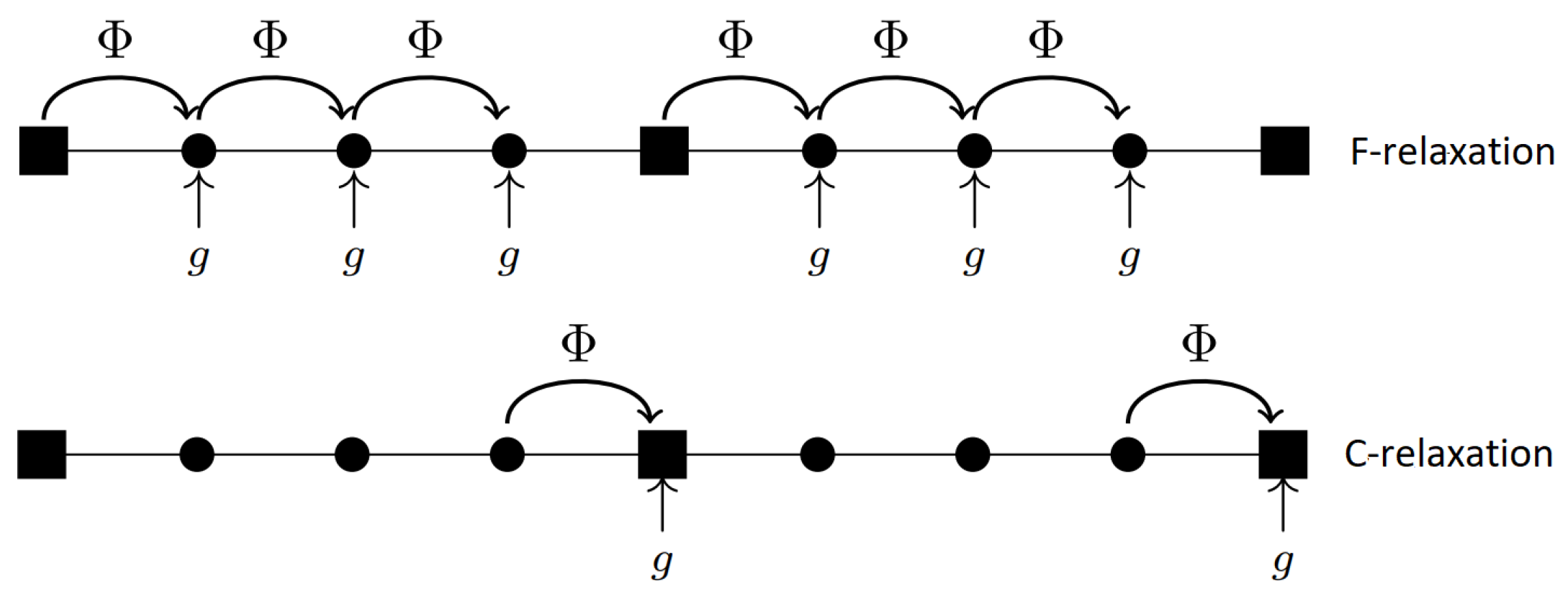
Figure 1. Illustration of F- and C-relaxation schemes.
Algorithms 18 00484 g001
Figure 2. Multigrid cycle types: V-cycle, W-cycle, and F-cycle.
Algorithms 18 00484 g002
Figure 3. Schematic concept of the refinement factor r.
Algorithms 18 00484 g003
Figure 4. Step-size sequences (y-axis) for different TOL values in the sequential and MGRIT-based adaptive methods over the given time intervals (x-axis) for the linear two-compartment dilution process problem (6).
Algorithms 18 00484 g004
Figure 5. Step-size sequences (y-axis) for different TOL values in the sequential and MGRIT-based adaptive methods over the given time intervals (x-axis) for the Lotka–Volterra problem (7).
Algorithms 18 00484 g005
Figure 6. Step-size sequences (y-axis) for different TOL values in the sequential and MGRIT-based adaptive methods over the given time intervals (x-axis) for the van der Pol problem (8).
Algorithms 18 00484 g006
Figure 7. The experiment shown in Figure 4 was re-simulated using the modified r m o d refinement factor with a compensating constant c = 0.4 .
Algorithms 18 00484 g007
Figure 8. The experiment shown in Figure 5 was re-simulated using the modified r m o d refinement factor with a compensating constant c = 0.4 .
Algorithms 18 00484 g008
Figure 9. The experiment shown in Figure 6 was re-simulated using the modified r m o d refinement factor with a compensating constant c = 0.4 .
Algorithms 18 00484 g009
Figure 10. Achieved accuracy (y-axis) versus tolerance (x-axis) for the linear two-compartment dilution process problem (6), using the three refinement-factor strategies.
Algorithms 18 00484 g010
Figure 11. Achieved accuracy (y-axis) versus tolerance (x-axis) for the Lotka–Volterra problem (7), using the three refinement-factor strategies.
Algorithms 18 00484 g011
Figure 12. Achieved accuracy (y-axis) versus tolerance (x-axis) for the van der Pol problem (8), using the three refinement-factor strategies.
Algorithms 18 00484 g012
Figure 13. Results for the linear (left column) and nonlinear (right column) diffusion Equation (10). Upper panel: step-size sequences (y-axis) over the given time interval (x-axis). Center panel: achieved accuracy (y-axis) versus tolerance (x-axis). Lower panel: runtime in seconds (y-axis) versus number of processors (x-axis).
Algorithms 18 00484 g013
Figure 14. Effect of the initial subinterval choice on the step-size sequence (y-axis) over the time interval (x-axis) for the Lotka–Volterra Equation (7).
Algorithms 18 00484 g014
Figure 15. Step-size sequences (y-axis) for the stiff van der Pol Equation (8) over the given time interval (x-axis). r m o d ( h e u r i s t i c s ) denotes our heuristic approach for a stiff problem.
Algorithms 18 00484 g015
Table 1. Number of time steps after the final refinement for different TOL values, using refinement factors r and r m o d , for the ODE test problems (6)–(8).
ProblemTOL 10 5 10 7 10 9 10 11 10 13
(6)r1281917183997 22 , 562
r m o d 1281696202828 13 , 076
(7)r2188554237 22 , 371 107 , 982
r m o d 1847543449 15 , 963 74 , 047
(8)r9313777 20 , 432 100 , 043 475 , 284
r m o d 7733070 14 , 090 65 , 258 302 , 692
Disclaimer/Publisher’s Note: The statements, opinions and data contained in all publications are solely those of the individual author(s) and contributor(s) and not of MDPI and/or the editor(s). MDPI and/or the editor(s) disclaim responsibility for any injury to people or property resulting from any ideas, methods, instructions or products referred to in the content.