Prediction of the Maximum and Minimum Prices of Stocks in the Stock Market Using a Hybrid Model Based on Stacking

Abstract

Predicting stock prices on stock markets is challenging due to the nonlinear and nonstationary nature of financial markets. This study presents a hybrid model based on integrated machine learning (ML) techniques—neural networks, support vector regression (SVR), and decision trees—that uses the stacking method to estimate the next day’s maximum and minimum stock prices. The model’s performance was evaluated using three data sets: Brazil’s São Paulo Stock Exchange (iBovespa)—Companhia Energética do Rio Grande do Norte (CSRN) and CPFL Energia (CPFE)—and one from the New York Stock Exchange (NYSE), the Dow Jones Industrial Average (DJI). The datasets covered the following time periods: CSRN and CPFE from 1 January 2008 to 30 September 2013, and DJI from 3 December 2018 to 31 August 2024. For the CSRN ensemble, the hybrid model achieved a mean absolute percentage error (MAPE) of 0.197% for maximum price and 0.224% for minimum price, outperforming results from the literature. For the CPFE set, the model showed a MAPE of 0.834% for the maximum price and 0.937% for the minimum price, demonstrating comparable accuracy. The model obtained a MAPE of 0.439% for the DJI set for maximum price and 0.474% for minimum price, evidencing its applicability across different market contexts. These results suggest that the proposed hybrid approach offers a robust alternative for stock price prediction by overcoming the limitations of using a single ML technique.

1. Introduction

Predicting stock prices on stock exchanges is a complex problem due to the highly nonlinear and non-stationary behavior of financial markets. Accurate predictions require extensive expertise and deep knowledge from professionals [1]. Accurate predictions can yield substantial economic benefits. For example, in 2024, 20% of the world’s 200 richest individuals will accumulate their wealth through finance and investments [2]. This financial potential motivates investors to seek methods for estimating future stock prices to maximize profits and reduce losses.

To date, research on daily stock-exchange price prediction can be grouped into five main lines of inquiry. First, studies that focus on stock indices—indicators of the aggregated value of the whole market or of specific sectors [3]—have sought to anticipate whether an index will rise or fall [4,5,6], its closing level [7,8,9], and even its intraday peak [10]. Second, a substantial body of work targets individual stock prices, forecasting their closing quotations [7,10,11,12,13,14] as well as their daily minima and maxima [15]. Third, researchers address stock price trends, classifying whether a given share is likely to appreciate or depreciate in the following session [12,16,17,18]. Fourth, a set of decision-support models for investors has emerged: some aggregate return, profit, and risk into a weighted score [19], while others generate buy/hold/sell signals over horizons of one to six days [20]. Finally, attention has turned to cryptocurrencies, with Bitcoin in particular inspiring models that predict its future USD exchange rate and trend direction [21]. While most existing studies focus on predicting closing prices or general market direction, [15] is one of the few that targets both maximum and minimum daily prices, which aligns closely with the objective of this study.

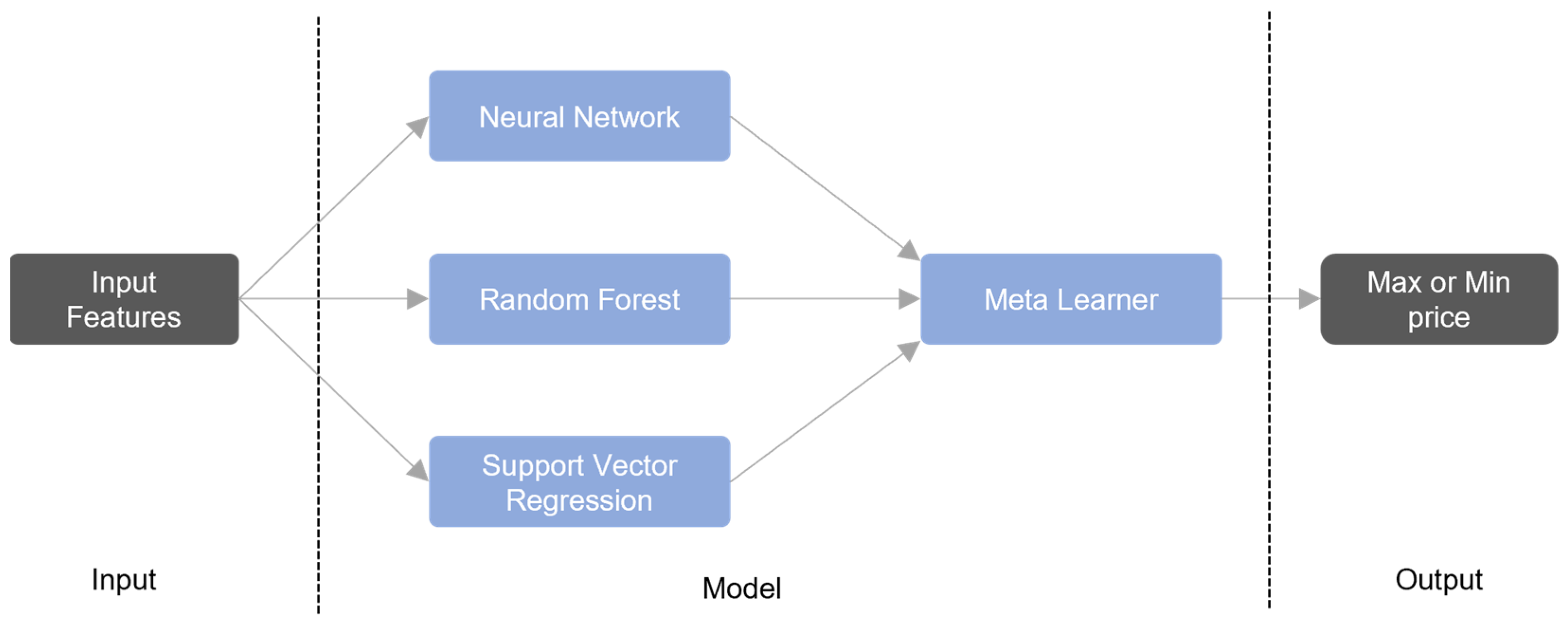
Traditional ML and deep-learning (DL) approaches often perform inconsistently across data sets. To mitigate this limitation, recent studies employ stacking ensembles instead of a single ML or DL model [22,23,24,25]. In stacking, several base (“weak”) learners are trained in parallel, and their predictions, together with the true labels, feed a meta-learner that learns how to combine them optimally, thereby improving overall accuracy [26,27]. Although stacking has been used in financial forecasting, most studies focus on predicting closing prices or binary movement direction. In contrast, this study focuses on predicting both the maximum and minimum daily stock prices using a structured hybrid ensemble. Furthermore, we combine neural networks, SVR, and decision trees in a specific configuration optimized for performance consistency across multiple datasets. This design, combined with the cross-market application to both Brazilian stocks and a U.S. index, represents a novel empirical contribution.

This research builds upon the results presented in the bachelor’s thesis of Sebastian Tuesta, defended at the Universidad Nacional Mayor de San Marcos (UNMSM) in 2025. The current study extends his preliminary work by incorporating additional financial indicators, refining the hybrid model architecture based on stacking techniques, and evaluating its predictive performance across different stock markets, including both national and international indices.

2. Materials and Methods

We propose a method for predicting the next day’s maximum and minimum stock price using a stacking-based hybrid model of ML models. The approach consists of four main stages: Data Collection, Preprocessing, Feature Selection, and the Hybrid Predictive Model (Figure 1).

2.1. Dataset Recopilation

In this stage, historical data were collected for each stock to be predicted, including opening, closing, maximum, and minimum prices. We used datasets from the literature, detailed in

Table 1. Datasets found in the literature.

Company	Ticker	Period	Stock Exchange
Companhia Energética do Rio Grande do Norte—COSERN	CSRN3.SA	1 January 2008–30 September 2013	Sao Paulo—iBovespa
Companhia Energética CPFL ENERGIAON	CPFE3.SA	1 January 2008–30 September 2013
Dow Jones Index	DJI	3 December 2018–31 August 2024	New York—NYSE

, which include two specific stocks, CSRN3.SA [15] and CPFE3.SA [15], and the DJI index [28] for benchmarking purposes. The same dates as in previous studies were used for the stock data to enable direct comparisons. The DJI index was included to assess the versatility of the proposed model.

Although only two individual stocks (CSRN3.SA and CPFE3.SA) were used, their selection was based on their frequent appearance in benchmark studies such as [15], allowing direct methodological comparison. We acknowledge, however, that the use of only two stocks limits the generalizability of our findings. To partially mitigate this, the DJI index was included to provide a broader market perspective.

2.2. Preprocessing

Data preprocessing included several key substages to ensure data quality and consistency:

• Non-Trading Days: Records corresponding to non-trading days were removed (i.e., there are no records for opening, closing, maximum, or minimum prices on these days).
• Feature Engineering: The following features were calculated: The opening price on the day to be predicted and the opening, closing, maximum, and minimum prices for the previous five days. Additionally, weighted moving averages (WMA) over a 30-calendar-day range (w-30) [15] were generated for opening, closing, maximum, and minimum prices. Only the five most recent daily prices and a weighted moving average (WMA) were used as input features. This minimalist configuration was chosen to avoid overfitting given the dataset size and to isolate the contribution of model architecture from additional feature engineering.
• Normalization: Data were normalized using the min–max normalization technique [29] to reduce the impact of different scales and improve the model accuracy.

2.3. Feature Selection

We used Pearson’s correlation coefficient [15] to select the most relevant features to identify the variables with the highest correlation to the next day’s maximum and minimum prices. This correlation analysis helps reduce the feature set, focusing on the model on the attributes that have the greatest influence on the predictions.

2.4. Prediction Model

The predictive model uses a hybrid approach based on the stacking technique. To date, only three peer-reviewed studies explicitly address the prediction of maximum or minimum stock prices as the target variable [10,15,21]. Other recent works—such as those by Priyatno et al. [30], Li et al. [31], and Dhyani et al. [32]—use modern algorithms (e.g., Random Forest, HFD-CNN-LSTM, Google Trend + ML) but focus on closing prices; high and low values are only used as input features.

Hybrid models are more accurate for price prediction compared with individual models [20,33,34,35,36]. According to [37], combining multiple learners within an ensemble improves predictive accuracy through effective aggregation mechanisms, reduces uncertainty when the optimal standalone model is unknown, and decreases forecast errors by leveraging the complementary strengths of diverse algorithms.

However, hybrid models also present disadvantages, such as the complexity involved in hyperparameter tuning and the increased computational cost [38,39]. These limitations remain relevant today, as confirmed by recent studies. Khan et al. [40] emphasize that stacking schemes “require extensive hyper-parameter tuning” and are “computationally expensive,” while Li and Wang [41] propose Bayesian optimization specifically to reduce tuning overhead in multi-stage stacking ensembles.

In the proposed model, neural networks, random forest, and SVR are used as base models or “weak learners,” while an additional neural network acts as a meta-model or “meta-learner” to combine their predictions (see Figure 2). Unlike other approaches, such as [21], which select the best-performing individual model, our method uses a meta-model that weighs and optimizes the outputs from each base technique.

3. Model Evaluation and Implementation

3.1. Walk-Forward Validation

Cross-validation is the most commonly used ML method for comparing algorithms [42]. Nonetheless, in scenarios where the order of data is essential, like time series, this approach is inappropriate [43]. In this instance, the walk-forward validation approach, noted in [44], is implemented, which is especially beneficial for time-series models.

In this approach, the training set size is fixed but shifts one observation forward in each iteration, thus preserving the temporal sequence. This method enables the evaluation of the model’s capacity to forecast outcomes using data that adhere to a natural time sequence. In this study, 75% of the data were used for training and 15% for validation. Further details are provided in Section 4. Figure 3 displays the data split utilized in this validation process.

3.2. Mean Absolute Percentage Error

The MAPE, a commonly used error metric for time series models, was used to evaluate the accuracy of the proposed model’s predictions. The formula for MAPE is as follows:

$$MAPE={\displaystyle \frac{100}{n}}\sum _{i=1}^n{\displaystyle \frac{{{Actual}_i-Forecast}_i}{{Actual}_i}}$$

(1)

where n is the total number of predictions, ${Actual}_i$ represents the actual value at time $i$, and ${Forecast}_i$ represents the forecasted value at time $i$.

3.3. Training and Implementation

To optimize the model’s performance, the parameters for each ML technique were calibrated based on values from previous studies—neural network parameters were adapted from [15] and those for random forest and SVR were adapted from [21]. The best result obtained from each weak model was then used in the hybrid model, in which the meta-learner (another neural network) was calibrated.

Table 2. Evaluated hyperparameters for each model.

Model	Parameter	Value
Support Vector Regression	Gamma	0.1, 0.2, 0.3, 0.4, 0.5
	Epsilon	0.1, 0.2, 0.3, 0.4, 0.5
	C	1, 2, 3, 4, 5, 6, 7, 8, 9, 10
	Kernel	Polynomial Degree 1, Polynomial Degree 2, Polynomial Degree 3, Linear, Sigmoid, RBF
Neural Network	Epochs	250
	Hidden Layers	1
	Hidden Layer Neurons	5, 10, 15, 20
	Regularization	Early Stopping
Random Forest	Trees	10, 20, 30, 40, 50, 100

shows the evaluated hyperparameter values for each model.

The key hyperparameters for SVR include the following: Gamma (γ), which defines the influence of a single training example; Epsilon (ε), which specifies the margin of tolerance where no penalty is given to errors; C, a regularization parameter that controls the trade-off between training error and model complexity; and the Kernel, which determines the function used to map data into higher-dimensional space (e.g., linear, polynomial, radial basis function). These parameters were tuned to optimize performance on each dataset.

Early stopping with a patience of 10 epochs was applied during training, allowing the process to stop if no improvement was observed after 10 consecutive epochs. Each epoch corresponds to one complete pass through the training dataset, with a default batch size of 32 samples per iteration. Note that the length of each dataset may vary, which affects the exact duration of an epoch. This helps prevent overfitting. In the case of the random forest, different numbers of trees were tried to achieve a balance between accuracy and computational efficiency. Finally, the SVR parameters were adjusted by exploring different values for gamma, epsilon, C, and various kernel types to adapt the model to the complexities of other datasets.

4. Results

This section presents the prediction results obtained for the CSRN and CPFE datasets, following the approach presented in [15]. In addition, the results are compared with those obtained from the DJI dataset to evaluate the model’s applicability across different contexts. For the experiments, the following aspects were considered:

• Data Split: 75% of the data were used for training and 25% for testing.
• MAPE Calculation: Actual and predicted values were denormalized during the MAPE calculation to avoid issues associated with normalized values of 0, which can occur when the actual value is the minimum in the dataset. Denormalization converts the values back to their original scales, ensuring that the error metric reflects meaningful differences and avoids division-by-zero errors.
• Feature Selection: The five features with the highest Pearson coefficients were selected, including the opening price, the previous day’s maximum price, the previous day’s minimum price, the previous day’s closing price, and the previous day’s opening price.

The results shown in

Table 3. Prediction results for the minimum price of the CSRN3 stock (five selected features).

Model	Parameters	MAPE (%)	RMSE	MAE	Directional Accuracy
Support Vector Regression	Kernel = Polynomial degree 1, C = 9, Epsilon = 0.1, Gamma = 0.3	0.971	0.108	0.098	0.929
Neural Networks	Epochs = 250, Hidden Layer Neurons = 5	0.248	0.038	0.03	0.049
Random Forest	Trees = 30	0.041	0.025	0.004	0.887
Hybrid Model	Epochs = 250, Hidden Layer Neurons = 3	0.224	0.04	0.025	0.057

,

Table 4. Prediction results for the maximum price of the CSRN3 stock (five selected features).

Model	Parameters	MAPE (%)	RMSE	MAE	Directional Accuracy
Support Vector Regression	Kernel = RBF, C = 5, Epsilon = 0.1, Gamma = 0.2	0.674	0.083	0.068	0.943
Neural Networks	Epochs = 250, Hidden Layer Neurons = 5	0.337	0.003	0.064	0.039
Random Forest	Trees = 90	0.049	0.028	0.005	0.865
Hybrid Model	Epochs = 250, Hidden Layer Neurons = 3	0.197	0.034	0.021	0.057

,

Table 5. Prediction results for the minimum price of the CPFE3 stock (five selected features).

Model	Parameters	MAPE (%)	RMSE	MAE	Directional Accuracy
Support Vector Regression	Kernel = Sigmoid, C = 5, Epsilon = 0.1, Gamma = 0.1	1.421	0.206	0.1697	0.596
Neural Networks	Epochs = 250, Hidden Layer Neurons = 5	0.746	0.121	0.089	0.652
Random Forest	Trees = 100	0.864	0.131	0.102	0.582
Hybrid Model	Epochs = 250, Hidden Layer Neurons = 3	0.937	0.145	0.113	0.574

,

Table 6. Prediction results for the maximum price of the CPFE3 stock (five selected features).

Model	Parameters	MAPE (%)	RMSE	MAE	Directional Accuracy
Support Vector Regression	Kernel = RBF, C = 2, Epsilon = 0.1, Gamma = 0.1	1.011	0.159	0.125	0.617
Neural Networks	Epochs = 250, Hidden Layer Neurons = 5	0.749	0.747	0.121	0.09
Random Forest	Trees = 100	0.754	0.118	0.094	0.666
Hybrid Model	Epochs = 250, Hidden Layer Neurons = 3	0.834	0.131	0.104	0.666

,

Table 7. Prediction results for the minimum price of the Dow Jones index (five selected features).

Model	Parameters	MAPE (%)	RMSE	MAE	Directional Accuracy
Support Vector Regression	Kernel = Polynomial degree 2, C = 8, Epsilon = 0.1, Gamma = 0.1	4.332	1796.5	1697.89	0.636
Neural Networks	Epochs = 250, Hidden Layer Neurons = 15	0.3695	187.12	147.89	0.727
Random Forest	Trees = 80	0.437	234.36	171.37	0.58
Hybrid Model	Epochs = 250, Hidden Layer Neurons = 3	0.474	246.93	186.08	0.57

and

Table 8. Prediction results for the maximum price of the Dow Jones index (five selected features).

Model	Parameters	MAPE (%)	RMSE	MAE	Directional Accuracy
Support Vector Regression	Kernel = Polynomial degree 2, C = 8, Epsilon = 0.1, Gamma = 0.1	2.738	1208.79	1087.49	0.678
Neural Networks	Epochs = 250, Hidden Layer Neurons = 20	0.328	175.35	133.75	0.68
Random Forest	Trees = 80	0.4001	212.69	158.72	0.643
Hybrid Model	Epochs = 250, Hidden Layer Neurons = 3	0.439	231.26	174.06	0.59

reflect the model’s optimal performance after parameter calibration.

5. Discussion and Conclusions

This paper introduces a stacking-based hybrid model to forecast a stock’s highest and lowest prices by employing three ML models as base learners and a meta-model for the final prediction. This method typically produces more consistent and precise outcomes than single ML models. While the current approach avoids sector-specific influences to simplify analysis, future research should explore the impact of industry-specific volatility on model performance. Including sectoral classification or volatility measures may provide deeper insights into how models generalize across heterogeneous financial environments.

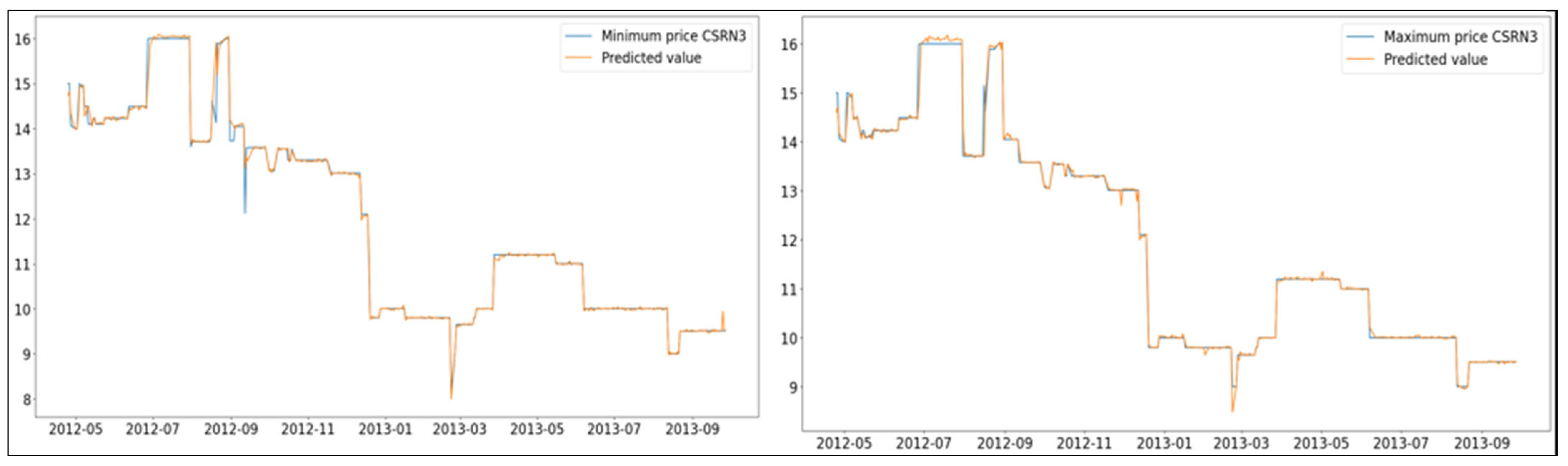
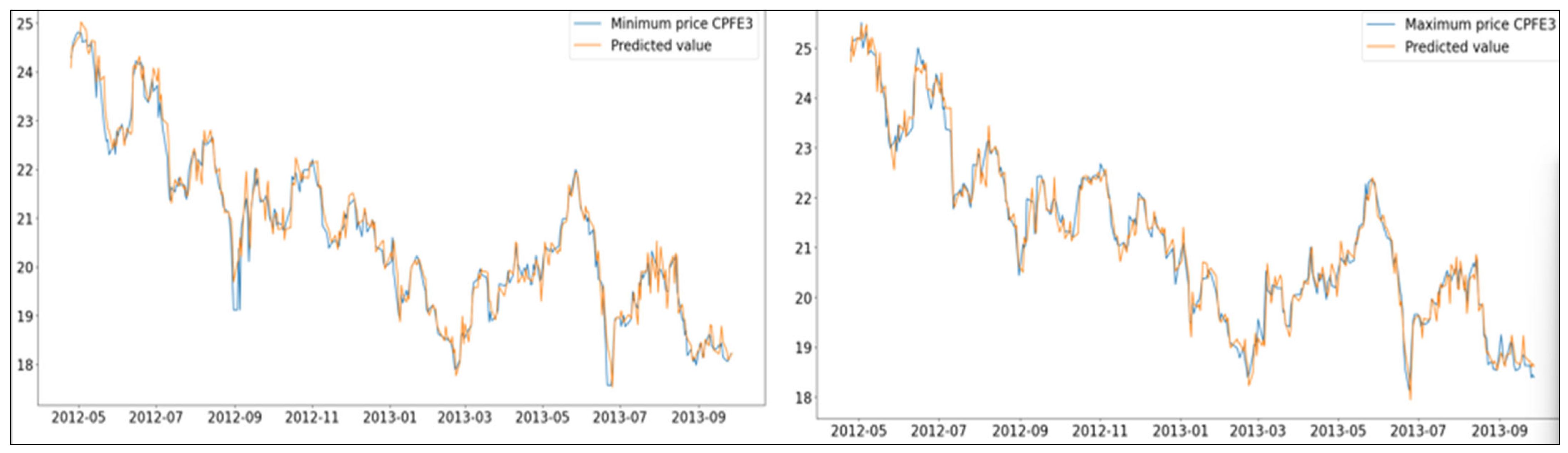
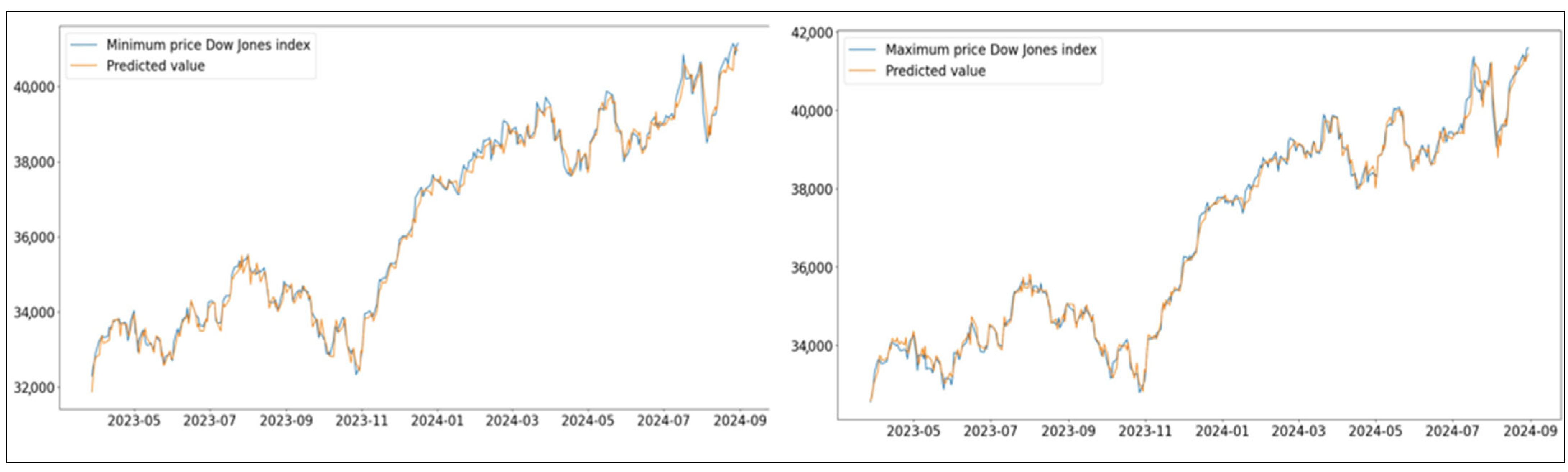
In three out of four instances, the results from the proposed model exceed those found in the reference study [15]. In the other case [15], its performance is similar to those of the state-of-the-art methods. Additionally, a further experiment validated the model’s competitiveness, attaining MAPEs < 1 for every stock and index examined (Figure 4, Figure 5 and Figure 6).In addition to MAPE, the model’s performance was also evaluated using RMSE, MAE, and directional accuracy, as reported in Table 3, Table 4, Table 5, Table 6, Table 7 and Table 8. These metrics provide complementary perspectives on prediction quality. RMSE and MAE assess the magnitudes of the prediction errors, while directional accuracy evaluates whether the predicted price movement direction (up or down) matches the actual movement. These results suggest that the hybrid model is capable of effectively adapting to the specific characteristics of the analyzed stock data and market index; however, due to the limited number of datasets, further validation is required to confirm its general applicability across a broader range of financial assets.

It is also important to note that this study did not include a direct comparison with recent deep-learning-based forecasting models such as long short-term memory (LSTM) networks or the Temporal Fusion Transformer (TFT). These methods have demonstrated strong predictive capabilities in time series tasks but were excluded here due to their considerably higher computational requirements. Future research should consider benchmarking the proposed hybrid model against such architectures to assess relative performance in terms of both accuracy and resource efficiency.

A key limitation of this study lies in the relatively narrow scope of the datasets used. Only two individual stocks (CSRN3.SA and CPFE3.SA) and one market index (DJI) were analyzed. Although these were selected based on their uses in prior benchmark studies to ensure methodological comparability, the limited dataset reduces the generalizability of the findings. Additionally, the time spans of the datasets are inconsistent: CSRN and CPFE cover the period from 2008 to 2013, while DJI spans 2018 to 2024. This temporal gap introduces macroeconomic and structural differences that may affect comparability and the interpretation of model performance across datasets. To partially address this, the DJI index was included to represent a broader international market context. Nevertheless, future research should incorporate a more diverse set of stocks from various sectors and global markets to further evaluate the robustness and scalability of the proposed hybrid model.

Another important consideration relates to the assumptions inherent in the proposed approach. The model assumes that short-term price dynamics can be effectively captured using only historical price data (five previous days) and weighted moving averages without incorporating technical indicators or external features. While this choice simplifies implementation and helps prevent overfitting, it also limits the model’s ability to capture sudden structural changes or external shocks. Future versions could benefit from integrating additional features, such as trading volume, volatility indices, or sectoral risk indicators.

This limited feature set is another notable constraint. By relying solely on historical prices and weighted moving averages (WMA), the model excludes potentially informative features such as trading volume, momentum-based indicators (e.g., RSI, MACD), and macroeconomic data. While this decision was made intentionally to control model complexity and focus on the stacking architecture, future studies should explore the effect of incorporating these variables on model accuracy and robustness.

While the proposed stacking model demonstrated strong predictive performance, its interpretability remains limited. As with many ensemble learning approaches, the internal decision logic of the model functions as a black box. This lack of transparency may hinder adoption in practical financial settings in which understanding the rationale behind predictions is essential. In future work, we recommend the use of SHAP (SHapley Additive exPlanations) values or permutation importance to identify the most influential input features and provide more interpretable insights into the model’s decision-making process.

Key factors affecting stock prices consist of news regarding company activities, mergers, and investments, as well as the macroeconomic variables of the nation where the company functions. In upcoming research, we suggest adding these variables to the model after assessing their correlations with stock prices and the trustworthiness of the information sources. Incorporating these variables might enhance prediction accuracy and account for the influence of external factors on stock prices.

In summary, although the proposed hybrid model has shown promising results, its evaluation remains limited to a narrow dataset and simplified input features. More extensive testing and enhancement are required before the model can be broadly applied. There remains considerable work to be accomplished in this field, particularly in improving generalization, interpretability, and real-time applicability across diverse market conditions.

References

1. Cheng, C.-H.; Yang, J.-H. Fuzzy time-series model based on rough set rule induction for forecasting stock price. Neurocomputing 2018, 302, 33–45. [Google Scholar] [CrossRef]
2. Forbes. The World’s Billonaries [Internet]. Forbes.com. 2025. Available online: https://www.forbes.com/real-time-billionaires/#39a8ac213d78 (accessed on 26 June 2025).
3. Lee, C.-F.; Lee, A.C. Encyclopedia of Finance; Springer: Boston, MA, USA, 2006; Available online: https://link.springer.com/referencework/10.1007/978-0-387-26336-6 (accessed on 26 June 2025).
4. Malagrino, L.S.; Roman, N.T.; Monteiro, A.M. Forecasting stock market index daily direction: A Bayesian Network approach. Expert Syst. Appl. 2018, 105, 11–22. [Google Scholar] [CrossRef]
5. Moews, B.; Herrmann, J.M.; Ibikunle, G. Lagged correlation-based deep learning for directional trend change prediction in financial time series. Expert Syst. Appl. 2019, 120, 197–206. [Google Scholar] [CrossRef]
6. Milke, V.; Luca, C.; Wilson, G.B. Reduction of financial tick big data for intraday trading. Expert Syst. 2024, 41, e13537. [Google Scholar] [CrossRef]
7. Xiao, J.; Zhu, X.; Huang, C.; Yang, X.; Wen, F.; Zhong, M. A New Approach for Stock Price Analysis and Prediction Based on SSA and SVM. Int. J. Inf. Technol. Decis. Mak. 2019, 18, 287–310. [Google Scholar] [CrossRef]
8. Yang, H.-L.; Lin, H.-C. An Integrated Model Combined ARIMA, EMD with SVR for Stock Indices Forecasting. Int. J. Artif. Intell. Tools 2016, 25, 1650005. [Google Scholar] [CrossRef]
9. Zheng, J.; Tian, Y.; Luo, J.; Hong, T. A novel hybrid method based on kernel-free support vector regression for stock indices and price forecasting. J. Oper. Res. Soc. 2023, 74, 690–702. [Google Scholar] [CrossRef]
10. Zhang, N.; Lin, A.; Shang, P. Multidimensional k -nearest neighbor model based on EEMD for financial time series forecasting. Phys. A Stat. Mech. Its Appl. 2017, 477, 161–173. [Google Scholar] [CrossRef]
11. Göçken, M.; Özçalıcı, M.; Boru, A.; Dosdoğru, A.T. Stock price prediction using hybrid soft computing models incorporating parameter tuning and input variable selection. Neural Comput. Appl. 2019, 31, 577–592. [Google Scholar] [CrossRef]
12. Hu, H.; Tang, L.; Zhang, S.; Wang, H. Predicting the direction of stock markets using optimized neural networks with Google Trends. Neurocomputing 2018, 285, 188–195. [Google Scholar] [CrossRef]
13. Pan, Y.; Xiao, Z.; Wang, X.; Yang, D. A multiple support vector machine approach to stock index forecasting with mixed frequency sampling. Knowl. Based Syst. 2017, 122, 90–102. [Google Scholar] [CrossRef]
14. Prasanna, S.; Ezhilmaran, D. Association rule mining using enhanced apriori with modified GA for stock prediction. Int. J. Data Min. Model. Manag. 2016, 8, 195. [Google Scholar] [CrossRef]
15. Laboissiere, L.A.; Fernandes, R.A.S.; Lage, G.G. Maximum and minimum stock price forecasting of Brazilian power distribution companies based on artificial neural networks. Appl. Soft Comput. 2015, 35, 66–74. [Google Scholar] [CrossRef]
16. Lei, L. Wavelet Neural Network Prediction Method of Stock Price Trend Based on Rough Set Attribute Reduction. Appl. Soft Comput. 2018, 62, 923–932. [Google Scholar] [CrossRef]
17. Li, X.; Xie, H.; Wang, R.; Cai, Y.; Cao, J.; Wang, F.; Min, H.; Deng, X. Empirical analysis: Stock market prediction via extreme learning machine. Neural Comput. Appl. 2016, 27, 67–78. [Google Scholar] [CrossRef]
18. Sadaei, H.J.; Enayatifar, R.; Lee, M.H.; Mahmud, M. A hybrid model based on differential fuzzy logic relationships and imperialist competitive algorithm for stock market forecasting. Appl. Soft Comput. 2016, 40, 132–149. [Google Scholar] [CrossRef]
19. Liu, Y.-C.; Yeh, I.-C. Using mixture design and neural networks to build stock selection decision support systems. Neural Comput. Appl. 2017, 28, 521–535. [Google Scholar] [CrossRef]
20. Ahmadi, E.; Jasemi, M.; Monplaisir, L.; Nabavi, M.A.; Mahmoodi, A.; Amini Jam, P. New efficient hybrid candlestick technical analysis model for stock market timing on the basis of the Support Vector Machine and Heuristic Algorithms of Imperialist Competition and Genetic. Expert Syst. Appl. 2018, 94, 21–31. [Google Scholar] [CrossRef]
21. Mallqui, D.C.A.; Fernandes, R.A.S. Predicting the direction, maximum, minimum and closing prices of daily Bitcoin exchange rate using machine learning techniques. Appl. Soft Comput. 2019, 75, 596–606. [Google Scholar] [CrossRef]
22. Zhang, Y.; Liu, J.; Shen, W. A Review of Ensemble Learning Algorithms Used in Remote Sensing Applications. Appl. Sci. 2022, 12, 8654. [Google Scholar] [CrossRef]
23. Wang, G.; Hao, J.; Ma, J.; Jiang, H. A comparative assessment of ensemble learning for credit scoring. Expert Syst. Appl. 2011, 38, 223–230. [Google Scholar] [CrossRef]
24. Liu, C.; Li, S.; Shi, L. A stock price manipulation detecting model with ensemble learning. Expert Syst. Appl. 2024, 248, 123479. [Google Scholar] [CrossRef]
25. Su, I.; Lin, P.L.; Chung, Y.; Lee, C. Forecasting of Taiwan’s weighted stock Price index based on machine learning. Expert Syst. 2023, 40, e13408. [Google Scholar] [CrossRef]
26. Yang, Y.; Lv, H.; Chen, N. A Survey on ensemble learning under the era of deep learning. Artif. Intell. Rev. 2023, 56, 5545–5589. [Google Scholar] [CrossRef]
27. Cao, Y.; Geddes, T.A.; Yang, J.Y.H.; Yang, P. Ensemble deep learning in bioinformatics. Nat. Mach. Intell. 2020, 2, 500–508. [Google Scholar] [CrossRef]
28. Golovachev, S. Forecasting the U.S. Stock Market via Levenberg-Marquardt and Haken Artificial Neural Networks Using ICA&PCA Pre-processing Techniques; Springer: Berlin/Heidelberg, Germany, 2011; pp. 351–357. [Google Scholar]
29. Akanbi, O.A.; Amiri, I.S.; Fazeldehkordi, E. Feature Extraction. In A Machine-Learning Approach to Phishing Detection and Defense; Elsevier: Amsterdam, The Netherlands, 2015; pp. 45–54. [Google Scholar]
30. Priyatno, A.M.; Ningsih, L.; Noor, M. Harnessing Machine Learning for Stock Price Prediction with Random Forest and Simple Moving Average Techniques. J. Eng. Sci. Appl. 2024, 1, 1–8. [Google Scholar] [CrossRef]
31. Li, Y.; Chen, L.; Sun, C.; Liu, G.; Chen, C.; Zhang, Y. Accurate Stock Price Forecasting Based on Deep Learning and Hierarchical Frequency Decomposition. IEEE Access 2024, 12, 49878–49894. [Google Scholar] [CrossRef]
32. Dhyani, B.; Bisht, S.; Sharma, A.; Prakash, C.; Tiwari, R. Stock Price Forecasting Using NASDAQ and Google Trend. In Proceedings of the 2024 Second International Conference on Advanced Computing & Communication Technologies (ICACCTech), Sonipat, India, 16–17 November 2024; IEEE: Piscataway Township, NJ, USA, 2024; pp. 244–249. [Google Scholar]
33. Mahmoodi, A.; Hashemi, L.; Mahmoodi, A.; Mahmoodi, B.; Jasemi, M. Novel comparative methodology of hybrid support vector machine with meta-heuristic algorithms to develop an integrated candlestick technical analysis model. J. Cap. Mark. Stud. 2024, 8, 67–94. [Google Scholar] [CrossRef]
34. Ebadati, E.O.M.; Mortazavi, T.M. An efficient hybrid machine learning method for time series stock market forecasting. Neural Netw. World 2018, 28, 41–55. [Google Scholar] [CrossRef]
35. Jia, Y.; Anaissi, A.; Suleiman, B. ResNLS: An improved model for stock price forecasting. Comput. Intell. 2024, 40, e12608. [Google Scholar] [CrossRef]
36. Zolfagharinia, H.; Najafi, M.; Rizvi, S.; Haghighi, A. Unleashing the Power of Tweets and News in Stock-Price Prediction Using Machine-Learning Techniques. Algorithms 2024, 17, 234. [Google Scholar] [CrossRef]
37. Allende, H.; Valle, C. Ensemble Methods for Time Series Forecasting. Stud. Fuzziness Soft Comput. 2017, 349, 217–232. [Google Scholar]
38. Anifowose, F.; Labadin, J.; Abdulraheem, A. Improving the prediction of petroleum reservoir characterization with a stacked generalization ensemble model of support vector machines. Appl. Soft Comput. 2015, 26, 483–496. [Google Scholar] [CrossRef]
39. Qureshi, A.S.; Khan, A.; Zameer, A.; Usman, A. Wind power prediction using deep neural network based meta regression and transfer learning. Appl. Soft Comput. 2017, 58, 742–755. [Google Scholar] [CrossRef]
40. Khan, A.A.; Chaudhari, O.; Chandra, R. A review of ensemble learning and data augmentation models for class imbalanced problems: Combination, implementation and evaluation. Expert Syst. Appl. 2024, 244, 122778. [Google Scholar] [CrossRef]
41. Li, Q.; Wang, X. Bayesian optimization of stacking ensemble learning model for HPC compressive strength prediction. Expert Syst. Appl. 2025, 288, 128281. [Google Scholar] [CrossRef]
42. Refaeilzadeh, P.; Tang, L.; Liu, H. Cross-Validation. In Encyclopedia of Database Systems; Springer: Boston, MA, USA, 2009; pp. 532–538. [Google Scholar]
43. Petropoulos, F.; Apiletti, D.; Assimakopoulos, V.; Babai, M.Z.; Barrow, D.K.; Ben Taieb, S.; Bergmeir, C.; Bessa, R.J.; Bijak, J.; Boylan, J.E.; et al. Forecasting: Theory and practice. Int. J. Forecast. 2022, 38, 705–871. [Google Scholar] [CrossRef]
44. Wang, S.; Li, K.; Liu, Y.; Chen, Y.; Tang, X. VIX constant maturity futures trading strategy: A walk-forward machine learning study. PLoS ONE 2024, 19, e0302289. [Google Scholar] [CrossRef] [PubMed]
Figure 1. Components proposed for this work.
Algorithms 18 00471 g001
Figure 2. The same stacking architecture is trained separately to predict the maximum and minimum prices, resulting in two distinct models.
Algorithms 18 00471 g002
Figure 3. Walk-forward validation schema.
Algorithms 18 00471 g003
Figure 4. Prediction of CSRN3 stock prices: left: minimum and right: maximum.
Algorithms 18 00471 g004
Figure 5. Prediction of CPFE3 stock prices: left: minimum and right: maximum.
Algorithms 18 00471 g005
Figure 6. Prediction of Dow Jones Index prices: left: minimum and right: maximum.
Algorithms 18 00471 g006