Abstract
Ferroptosis, an iron-dependent form of regulated cell death, plays a critical role in various diseases. Accurate identification of ferroptosis-related proteins (FRPs) is essential for understanding their underlying mechanisms and developing targeted therapeutic strategies. Existing computational methods for FRP prediction often exhibit limited accuracy and suboptimal performance. In this study, we harnessed the power of pre-trained protein language models (PLMs) to develop a novel machine learning framework, termed PLM-FRP, which utilizes deep learning-derived features for FRP identification. By integrating ESM2 embeddings with traditional sequence-based features, PLM-FRP effectively captures complex evolutionary relationships and structural patterns within protein sequences, achieving a remarkable accuracy of 96.09% on the benchmark dataset and significantly outperforming previous state-of-the-art methods. We anticipate that PLM-FRP will serve as a powerful computational tool for FRP annotation and facilitate deeper insights into ferroptosis mechanisms, ultimately advancing the development of ferroptosis-targeted therapeutics.
1. Introduction
Ferroptosis, a recently discovered form of regulated cell death characterized by iron-dependent lipid peroxidation [1], is implicated in a range of pathologies, including cancer [2], neurodegenerative disorders [3], and ischemia–reperfusion injury [4]. First defined by Dixon et al. [5], this process is driven by the accumulation of lipid peroxides, which is executed or inhibited by a class of proteins known as ferroptosis-related proteins (FRPs). Key examples include the suppressor GPX4 (UniProtKB P36969) [6], the driver ACSL4 (UniProtKB O60488) [7], and various iron-regulating proteins [8]. Consequently, the accurate identification of FRPs is a critical step for advancing therapeutic strategies, such as targeting ferroptosis suppressor protein 1 (FSP1, UniProtKB Q96NN9) to overcome treatment resistance [9].
However, traditional experimental methods for identifying and characterizing FRPs, such as gene knockout or overexpression studies, are often time-consuming, laborious, and resource-intensive. Computational methods, particularly those based on machine learning, offer a promising alternative for large-scale and efficient FRP prediction. To our knowledge, only one computational tool, FRP-XGBoost [10], has been specifically developed for this purpose. The authors of that study employed four types of sequence-based features and evaluated six traditional machine learning classifiers. Although FRP-XGBoost achieved satisfactory accuracy in 10-fold cross-validation, its performance on the independent test set was notably lower, indicating a need for more robust predictive models. This performance gap suggests that there is significant room for improvement through the design of more advanced feature descriptors and more powerful classification algorithms.
Recent years have witnessed remarkable advancements in protein bioinformatics, largely driven by the development of deep learning models, particularly pre-trained protein language models (PLMs). Models like ESM2 [11] have revolutionized various protein prediction tasks, including the identification of disease-related proteins [12]. Trained on vast datasets of protein sequences, these powerful models excel at learning intricate patterns and long-range dependencies, leading to significant improvements in prediction accuracy over traditional computational methods. Despite their immense promise, the application of PLMs to FRP prediction remains largely unexplored. The prior work, FRP-XGBoost, relied on conventional machine learning and did not leverage the rich, contextual embeddings offered by PLMs. This represents a significant opportunity to enhance the accuracy and efficiency of FRP identification.
In this study, we introduce PLM-FRP, a novel machine learning framework designed for the accurate identification of FRPs by harnessing the power of PLMs. Our framework integrates traditional sequence-based features (dipeptide composition and DDE) with advanced contextual embeddings from the ESM2 model. These comprehensive features are then supplied to an optimized XGBoost classifier for robust prediction. The overall workflow of PLM-FRP is illustrated in Figure 1. By combining these diverse feature sets, PLM-FRP captures a holistic view of protein properties, from local sequence composition to global evolutionary and structural information. We demonstrate that our model significantly outperforms existing methods on a benchmark dataset, achieving state-of-the-art accuracy and representing a 4% improvement over the previous best-performing method [10]. This advance holds immense potential to accelerate ferroptosis research by enabling the rapid annotation of novel FRPs, thereby facilitating a deeper understanding of their signaling pathways and paving the way for new targeted therapies.
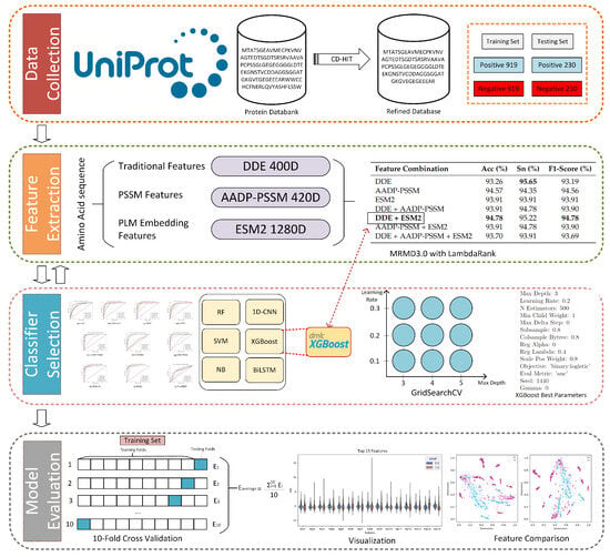
Figure 1.
Workflow of the proposed PLM-FRP model.
2. Materials and Methods
2.1. Benchmark Dataset
The performance of our proposed model was evaluated using the benchmark dataset curated by Lin et al. [10]. This dataset was meticulously constructed by sourcing known FRPs—including drivers, suppressors, and markers—from the Ferroptosis Database (FerrDb V2) [13]. For the negative set, non-FRPs were carefully selected from the Universal Protein Knowledgebase (UniProtKB) [14] under stringent criteria, ensuring a balanced and representative dataset by excluding any proteins with known links to ferroptosis.
To mitigate potential bias from sequence homology, the CD-HIT tool was employed to remove redundant entries with a similarity threshold of 90%. The final, non-redundant dataset consists of 1149 positive (FRPs) and 1149 negative (non-FRPs) sequences. For robust model validation, this dataset was partitioned into a training set of 1840 proteins (80%) and an independent test set of 460 proteins (20%), maintaining a balanced class distribution in both subsets. This rigorous preparation process yields a high-quality benchmark for developing and evaluating FRP prediction models.
2.2. Traditional Feature Extraction
In this study, we employed four widely used traditional feature extraction methods to represent protein sequences:
(i) Amino acid composition (AAC) [15] calculates the frequency of each amino acid in a protein sequence, resulting in a 20-dimensional feature vector.
where is the number of occurrences of amino acid i and N is the total number of amino acids in the sequence.
(ii) Composition of k-Spaced Amino Acid Pairs (CKSAAP) [16] captures the composition of amino acid pairs separated by k residues, providing information regarding short-range interactions.
where is the number of occurrences of pair separated by k residues and is the total number of possible pairs in the sequence.
(iii) Dipeptide Deviation from Expected Mean (DDE) [17] measures the deviation of observed dipeptide frequencies from expected mean frequencies, reflecting preferences in local amino acid order.
where is the observed frequency of dipeptide , is the expected frequency of dipeptide , and is the standard deviation of dipeptide .
(iv) Grouped Tripeptide Composition (GTPC) [18] groups amino acids based on physicochemical properties and calculates the frequency of tripeptides formed by these groups.
where is the number of occurrences of tripeptides formed by groups , , and , and is the total number of tripeptides in the sequence.
2.3. PSSM Feature Extraction
Evolutionary information plays a vital role in deciphering protein function and structure. To leverage this evolutionary information, the PSI-BLAST tool [19] was used to generate a Position-Specific Scoring Matrix (PSSM) for each protein sequence. Following standard bioinformatics practice, PSI-BLAST was run against the comprehensive NCBI non-redundant (NR) protein database. The search parameters were set to three iterations (iter = 3) with an E-value threshold of 0.001 (E = 0.001), which are commonly used settings for generating robust PSSMs. The PSSM captures the evolutionary conservation of amino acids at each position, offering a more informative representation compared to the raw amino acid sequence. In this study, three PSSM-based features were employed to comprehensively capture evolutionary information from protein sequences and enhance classifier performance.
2.3.1. AADP-PSSM
The AADP-PSSM [20] method combines AAC and dipeptide composition (DPC) features derived from the normalized PSSMs.
AAC-PSSM: For each protein sequence, AAC-PSSM is calculated by averaging the normalized PSSM values across all positions for each of the 20 standard amino acids, resulting in a 20-dimensional feature vector.
where L is the length of the protein sequence, and is the normalized PSSM value at position j for amino acid type i.
DPC-PSSM: DPC-PSSM captures the frequency of dipeptide combinations within the evolutionary context. It is calculated by averaging the product of normalized PSSM values for adjacent amino acid pairs across all positions, resulting in a 400-dimensional feature vector.
where L is the length of the protein sequence and and are the normalized PSSM values at positions k and for amino acid types i and j, respectively.
The final AADP-PSSM feature vector is a concatenation of the AAC-PSSM and DPC-PSSM features, resulting in a 420-dimensional feature vector.
2.3.2. S-FPSSM
The S-FPSSM [21] (Sum-Frequency PSSM) method generates a 400-dimensional feature vector derived from the FPSSM matrix by row transformation. In this method, the FPSSM is a matrix where the negative values from the original PSSM have been filtered out (set to zero).
The S-FPSSM vector is constructed by considering each of the 20 amino acids (rows in a PSSM) across the length of the protein sequence. Each element of the vector is calculated based on the FPSSM and an indicator function that considers amino acid matches. This vector represents a 400-dimensional feature.
The value of is calculated as follows:
where
- L is the length of the protein sequence.
- represents the element in the ith row and jth column of the FPSSM matrix. This means it is the positive part of the PSSM for the ith amino acid type at position j.
- is an indicator function defined as follows:
- represents the amino acid at position j in the original protein sequence.
- represents the ith amino acid type in the standard amino acid order. This indicates whether the amino acid at position j in the protein sequence corresponds to the ith amino acid type.
2.3.3. k-Separated Bigram-PSSM (KSB-PSSM)
This method extends the DPC-PSSM concept by considering amino acid pairs separated by k residues (k-spaced pairs or k-separated bigrams) within the PSSM profile [22]. It calculates the transfer probability of k-spaced amino acid pairs across all positions, resulting in a 400-dimensional feature vector.
The KSB-PSSM feature vector is a 400-dimensional vector, where each element is denoted as and corresponds to the transfer probability of a pair of amino acids, i and j, separated by k residues. This is represented as follows:
The calculation of a single element is as follows:
where L represents the protein sequence length and and represent the normalized PSSM values at positions t and for amino acid types i and j, respectively.
By employing these three PSSM-based feature extraction methods, we aimed to capture a diverse range of evolutionary information embedded in the PSSM profiles, including overall amino acid composition, short-range dipeptide interactions, and long-range evolutionary dependencies, providing a comprehensive representation of protein sequences for FRP prediction.
2.4. PLM Feature Embedding
To capture rich contextual information and evolutionary relationships inherent in protein sequences, we utilized pre-trained PLMs such as ESM-1b, ESM2, and ProtBert. These models are all based on the Transformer architecture [23]. PLMs, trained on extensive protein sequence datasets, have shown significant success in capturing complex patterns and evolutionary dependencies essential for understanding protein function [24].
ESM-1b and ESM2 are large-scale models, each comprising 33 Transformer layers and approximately 650 million parameters [11,25]. ProtBert, another prominent PLM, is derived from Google’s BERT model and pre-trained on a massive dataset of 100 million protein sequences [26]. This pre-training allows ProtBert to learn general representations of protein sequences, effectively capturing the "language" of proteins. The depth and capacity of these models (ESM-1b, ESM2, and ProtBert) enable them to effectively learn intricate patterns in protein sequences [27], capturing both local and long-range interactions vital for accurate protein function prediction.
Figure 2 schematically illustrates the process of extracting and aggregating protein features from these pre-trained language models. Specifically, as the sequence propagates through the Transformer layers, the model generates contextualized embeddings for each amino acid at each layer, capturing both the identity and the contextual information of each amino acid within the sequence [28]. This enables the model to discern the influence of neighboring amino acids on protein function. Hidden states from the last (33rd) layer of both ESM-1b and ESM2-650M models, and the output of the final layer for ProtBert, were extracted as feature representations for each protein sequence. Specifically, for each protein sequence, the embeddings of all amino acids from the last layer were averaged to produce a single, fixed-length feature vector. Both ESM-1b and ESM2 models yield 1280-dimensional feature vectors (embeddings) for each amino acid, and thus the mean embedding for an entire protein sequence also results in a 1280-dimensional vector. ProtBert, similarly, produces 1024-dimensional feature vectors for each amino acid, resulting in a 1024-dimensional mean embedding for the entire sequence.
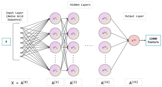
Figure 2.
Schematic illustration of feature extraction by aggregating layer-wise embeddings from PLMs (ESM-1b/ESM2/ProtBert) for protein representation.
Using these pre-trained PLMs, we extracted highly informative and contextualized representations of protein sequences, capturing intricate patterns and evolutionary dependencies essential for FRP prediction. The substantial parameter size and depth of ESM-1b, ESM2, and ProtBert enable them to directly learn complex representations from the data, outperforming traditional methods reliant on handcrafted features. This approach improves prediction accuracy by leveraging deep learning and large-scale pre-training to model the complex biological properties of protein sequences.
2.5. Feature Selection
MRMD3.0 [29], a robust dimensionality reduction tool employing an ensemble link analysis strategy, was used to identify the optimal feature subset. MRMD3.0 integrates multiple feature ranking algorithms, incorporating the PageRank algorithm, a well-established method for ranking nodes in a network based on their importance [30]. In the context of MRMD3.0, the PageRank algorithm is adapted to model features as nodes in a graph. The “importance” or “rank” of a feature node is then iteratively calculated based on its relevance to the target variable and its redundancy with other features. Features that are highly relevant to the target and less redundant with other high-ranking features receive higher PageRank scores, thereby contributing to a more effective feature ranking. The feature ranking algorithms included Information Gain, Gain Ratio, Gini Index, Chi-squared, ReliefF, minimum Redundancy Maximum Relevance (mRMR), and Mutual Information. By combining these algorithms, each with distinct strengths, MRMD3.0 generates a robust and comprehensive feature ranking.
The feature selection process in MRMD3.0 comprises two key steps. Initially, raw hybrid features are ranked based on importance scores calculated by the ensemble of ranking algorithms. Subsequently, a forward feature selection strategy, combined with 10-fold cross-validation, is used to iteratively add features to the model and assess its performance, measured by classification accuracy. The feature subset achieving the highest accuracy is selected as the optimal set [31]. This two-step strategy leverages the strengths of ensemble learning and PageRank, facilitating the identification of a robust and informative feature set for accurate FRP prediction.
Furthermore, an XGBoost classifier combined with LambdaRank, a ranking algorithm specifically designed for optimizing ranking tasks [32], was incorporated to complement MRMD3.0. While MRMD3.0 provides an initial robust feature subset, LambdaRank, integrated with XGBoost, serves as a secondary refinement step. It optimizes the feature ranking specifically for the classification task by leveraging gradient boosting to assign importance scores that directly improve the classifier’s performance. This enhanced feature selection process results in improved prediction accuracy and model robustness. This integrated approach ensures that the selected features are both informative and optimally ranked for the classification task [33].
2.6. Model Training
We employed a diverse set of machine learning algorithms, encompassing both traditional classifiers and deep learning models, to train our prediction models. This approach facilitated a thorough exploration of the strengths and limitations of each algorithm in capturing the intricate characteristics of FRPs.
2.6.1. Traditional Machine Learning Classifiers
We employed four widely adopted traditional machine learning classifiers to evaluate their effectiveness in predicting FRPs:
Support Vector Machine (SVM): A robust supervised learning algorithm that seeks to find the optimal hyperplane that best separates data into distinct classes [34]. By maximizing the margin between classes, SVM is effective in high-dimensional spaces. We employed the radial basis function (RBF) kernel, renowned for its ability to model non-linear relationships within the data.
Random Forest (RF): Random Forest (RF) is a popular ensemble learning method for classification and regression tasks in machine learning. It extends the decision trees by combining multiple trees to make predictions [35]. For classification, RF predicts the class label via majority voting among individual trees, where each tree’s prediction contributes to the final class with the most votes.
Naive Bayes (NB): A probabilistic classifier based on Bayes’ theorem, which operates under the assumption of conditional independence between features given the class label [36]. Despite its simplicity, Naive Bayes classifiers have demonstrated strong performance in various classification tasks, particularly with high-dimensional data.
eXtreme Gradient Boosting (XGBoost): A scalable and efficient implementation of gradient boosting machines, celebrated for its high accuracy and efficiency in handling structured data [37,38]. XGBoost builds an ensemble of weak predictive models, typically decision trees, in a stage-wise manner and optimizes a differentiable loss function.
These classifiers were implemented using the scikit-learn library (v0.24.2) in Python 3.10 [39]. Hyperparameters were optimized through grid search and cross-validation to ensure optimal performance for each classifier.
2.6.2. Deep Learning Models
To further explore the potential of deep learning in FRP prediction, we employed two advanced architectures: 1D Convolutional Neural Networks (1D-CNNs) and Bidirectional Long Short-Term Memory networks (BiLSTMs). These architectures were chosen due to their proven capabilities in handling sequential data, which is characteristic of protein sequences, and their ability to capture complex hierarchical and temporal dependencies, respectively. While simpler models like Multilayer Perceptrons (MLPs) or Artificial Neural Networks (ANNs) can also process sequential data, they typically lack the specialized architectural inductive biases that make 1D-CNNs and BiLSTMs particularly effective at extracting meaningful features from long and intricate sequences like proteins. Therefore, we focused on these more advanced deep learning models to maximize the predictive power for FRPs.
1D-CNNs are powerful architectures adept at processing sequential data such as protein sequences [40]. Our 1D-CNN architecture (Figure 3a) comprises convolutional layers, max-pooling layers, and fully connected layers, incorporating ReLU activation functions and dropout regularization to prevent overfitting. This design facilitates the extraction of hierarchical feature representations, capturing both local and global patterns within the sequences.
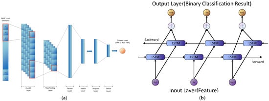
Figure 3.
Architectures of the proposed deep learning models for FRP prediction. (a) Architecture of the proposed 1D Convolutional Neural Network (1D-CNN) for FRP prediction. The model includes multiple convolutional and pooling layers to improve feature extraction, followed by fully connected layers and a sigmoid output layer for binary classification. (b) Architecture of the proposed Bidirectional Long Short-Term Memory (BiLSTM) network for FRP prediction. The model comprises multiple BiLSTM layers that process the input sequences bidirectionally, capturing long-range dependencies within protein sequences. These recurrent layers are followed by fully connected layers, and a sigmoid activation function is employed in the output layer for binary classification.
BiLSTM networks, a specialized variant of Recurrent Neural Networks (RNNs), are designed to capture long-range dependencies within sequential data [41]. BiLSTM processes sequences in both forward and backward directions, enabling it to learn comprehensive representations of the input sequences. Our BiLSTM architecture (Figure 3b) consists of two bidirectional LSTM layers followed by a fully connected layer, effectively capturing temporal dependencies and contextual information critical for accurate prediction [42].
For both 1D-CNN and BiLSTM models, we extensively utilized dropout layers (with a rate of 0.5) within the network architectures and implemented Early Stopping during training. Early Stopping monitored the validation loss, halting training when no further improvement was observed, thereby ensuring that the models generalized well to unseen data.
2.6.3. Hyperparameter Optimization and Cross-Validation
To ensure optimal performance for each classifier and deep learning model, we employed grid search to systematically explore a range of hyperparameter values and identify the best configuration [43]. Grid search involves exhaustively searching through a specified subset of hyperparameters, allowing us to fine-tune the models for optimal performance [44]. We utilized 10-fold cross-validation, a robust technique that partitions the training data into ten folds [45]. In each iteration, nine folds were used for training the model, and the remaining fold was used for validation, rotating the folds to guarantee that each data point was used for validation exactly once. This approach mitigates the risk of overfitting and provides a reliable estimate of the model’s generalization ability.
Table 1 details the final set of hyperparameters chosen for each model following grid search and 10-fold cross-validation. By employing a diverse array of machine learning algorithms, optimizing their hyperparameters through systematic grid search, and utilizing robust cross-validation techniques, we aimed to develop highly accurate and generalizable prediction models for FRPs.

Table 1.
Hyperparameter search grid and optimal values for selected classifiers.
2.7. Model Evaluation
An objective assessment of the predictive performance of our classifiers was conducted using a 10-fold cross-validation approach. The dataset was divided into ten partitions, with nine partitions used for training and one for testing. This process was iterated ten times, and the average accuracy across these iterations was used as the final estimate of model performance.
To comprehensively evaluate the models, five commonly used metrics were employed: sensitivity (Sn), specificity (Sp), Matthews correlation coefficient (MCC), accuracy (Acc), and area under the receiver operating characteristic (ROC) curve (AUC). The formulas for these metrics are as follows:
Acc measures the proportion of correctly predicted samples over the total samples. Sn measures the proportion of actual positives correctly identified, also known as Recall. Sp measures the proportion of actual negatives correctly identified. MCC considers true and false positives and negatives to provide a balanced evaluation, while AUC indicates the model’s ability to distinguish between classes.
3. Results and Discussion
3.1. Classifier Selection
To evaluate the efficacy of various feature extraction methods in capturing the characteristics of FRPs, we assessed the performance of each feature representation using six distinct classifiers: SVM, XGBoost, RF, NB, 1D-CNN, and BiLSTM. Figure 4 presents the ROC curves for each feature set, with the corresponding AUC values provided in the legend.
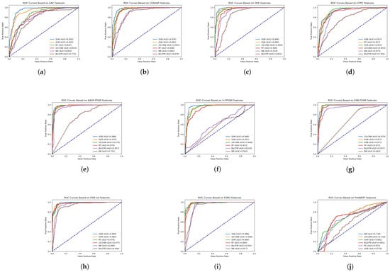
Figure 4.
ROC curves for various single-feature methods using six classifiers, with AUC values indicated in the legend. (a) AAC; (b) CKSAAP; (c) DDE; (d) GTPC; (e) AADP-PSSM; (f) S-FPSSM; (g) KSB-PSSM; (h) ESM-1b; (i) ESM2; (j) ProtBERT.
Analysis of the ROC curves and AUC values (Figure 4) revealed that SVM and XGBoost consistently delivered the highest performance across the various single-feature representations. This suggests their superior capability in discerning the complex patterns associated with FRPs. Furthermore, the DDE and ESM2 features consistently yielded high AUC values across multiple classifiers, demonstrating their strong discriminative power for distinguishing between FRPs and non-FRPs.
Based on these findings, we selected SVM and XGBoost for subsequent comparative analysis. Figure 5 provides a detailed performance comparison, based on classification accuracy, between the SVM and XGBoost classifiers across the different single-feature sets.
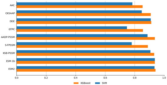
Figure 5.
Performance comparison between XGBoost and SVM.
As illustrated in Figure 5, the XGBoost classifier consistently outperformed SVM across most individual feature representations, achieving higher accuracy in 8 out of 10 cases. This superior performance indicates XGBoost’s enhanced capacity to effectively capture complex patterns and interactions within the feature spaces derived from these methods. The gradient boosting framework of XGBoost constructs an ensemble of weak predictive models—typically decision trees—in a stage-wise fashion while optimizing a differentiable loss function. This process enhances its ability to model non-linear relationships and feature interactions, making it particularly well-suited for the high-dimensional and complex nature of FRP prediction. Moreover, XGBoost’s built-in regularization techniques help prevent overfitting, further contributing to its robust performance. These findings validate our selection of XGBoost as the primary classifier for subsequent analyses and model development.
3.2. Performance Comparison with Hybrid Features
To explore the potential of integrating complementary features for enhancing prediction accuracy, a series of ablation experiments were conducted to evaluate the performance of different feature combinations. Initially, combinations of traditional features, PSSM-based features, and embeddings from large models like ESM-1b and ESM2 were tested. While these combinations improved prediction accuracy, strategic feature selection emphasizing evolutionary information and structural properties further enhanced performance. To systematically evaluate the contribution of each feature type, ablation experiments were performed using optimal traditional features, PSSM features, and large model embeddings. Specific combinations tested included traditional features alone, PSSM features alone, large model embeddings alone, and their pairwise combinations. It is noteworthy that among the tested large model embeddings, ProtBERT features (Figure 4j) showed comparatively lower performance than ESM2 for this task, leading us to prioritize ESM2 for further feature combinations. Results indicated that while each feature type individually contributed to prediction accuracy, their combinations offered complementary perspectives on protein sequence characteristics, leading to further enhancements.
As detailed in Table 2, the combination of DDE and ESM2 features achieved the highest performance across most evaluation metrics, with an accuracy of 94.78% and an MCC of 0.896. This result highlights the powerful synergy between traditional, sequence-derived statistics and modern, deep learning-based representations. The DDE feature effectively captures local compositional biases, while the ESM2 embeddings provide rich, context-aware information about global evolutionary and structural properties. This fusion of complementary information proved to be the most effective strategy, outperforming other combinations, including those incorporating PSSM-based features.

Table 2.
Performance of different feature combinations on the independent test set.
The DDE + ESM2 combination demonstrated the highest prediction accuracy, underscoring the importance of integrating features that provide complementary insights into protein sequences. The DDE feature encapsulates both amino acid composition and dipeptide composition within an evolutionary context, while the ESM2 embeddings capture detailed structural and functional information. This synergy between evolutionary and structural properties proved to be the most effective in our experiments.
In conclusion, our ablation study confirms that integrating DDE features with ESM2 embeddings creates a highly discriminative feature set for FRP prediction. This finding underscores the value of a hybrid approach, which leverages diverse feature types to capture a multifaceted view of protein sequences, ultimately leading to more accurate and robust predictive models.
3.3. Classification Results and Model Performance
Building upon the optimal DDE + ESM2 feature combination, we employed a LambdaRank-based feature selection strategy to further refine the feature set and enhance model performance. This advanced selection process identified a highly informative subset of features, effectively reducing dimensionality, mitigating the risk of overfitting, and improving model generalizability. Subsequently, we trained our final XGBoost classifier, previously identified as the top-performing algorithm, on this optimized feature subset. Figure 6 illustrates the relationship between the number of selected features and the corresponding classification accuracy.
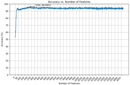
Figure 6.
The accuracy of selected features using the XGBoost classifier.
The final optimized feature set, derived from the DDE and ESM2 embeddings, resulted in a 216-dimensional input vector for the XGBoost classifier. To rigorously assess the model’s robustness and generalizability, we performed 10-fold cross-validation on the training set. The model achieved an impressive average accuracy of 96.52% across the 10 folds, with a peak accuracy of 97.26% in 1 fold. This consistently high performance across different data partitions underscores the model’s strong ability to generalize to unseen data, indicating its robustness and reliability.
The performance of our final model, named PLM-FRP, was validated on the independent test set. As shown in Table 3, PLM-FRP achieved a remarkable accuracy of 96.09%, significantly surpassing the performance of existing FRP prediction methods.

Table 3.
Comparison of various methods using traditional features and feature selection strategies.
These exceptional results, corroborated by the high accuracy in 10-fold cross-validation, highlight the power of combining PLM embeddings with a robust feature selection strategy to achieve state-of-the-art performance in FRP prediction. This approach not only improves prediction accuracy but also yields a more focused and interpretable model, enabling a deeper understanding of the features driving the prediction.
3.4. Model Interpretation
To elucidate the decision-making process of our final model, PLM-FRP, we employed SHapley Additive exPlanations (SHAP) [46]. The SHAP framework provides a robust method for interpreting machine learning models by quantifying the contribution of each feature to an individual prediction. By leveraging principles from cooperative game theory, SHAP fairly allocates the impact of each feature on the model’s output, thereby offering a comprehensive understanding of feature importance.
To visualize the feature space and the effectiveness of our selection strategy, we first employed t-Distributed Stochastic Neighbor Embedding (t-SNE) [47]. As shown in Figure 7, the t-SNE plots reveal a markedly improved separation between positive (FRPs) and negative (non-FRPs) samples after feature selection. This observation underscores the efficacy of our feature selection pipeline in identifying a highly discriminative feature subset that enhances the model’s ability to distinguish between the two classes. To further examine the relationships between the most predictive features, a correlation heatmap was also generated (Figure 8).
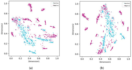
Figure 7.
Comparison before and after feature selection. (a) Before feature selection. (b) After feature selection.
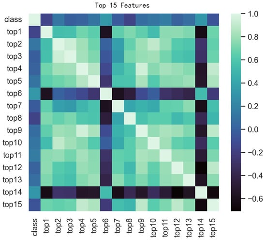
Figure 8.
Correlation heatmap of top 15 features and target variable.
To further analyze the impact of individual features, we generated a SHAP summary plot for the top 20 features from the optimized DDE + ESM2 combination (Figure 9). This plot illustrates both the magnitude and direction of each feature’s influence on the model’s output. Features with positive SHAP values push the prediction towards the FRP class, while negative values push it towards the non-FRP class. The color intensity indicates the feature’s value, providing deeper insight into its behavior.
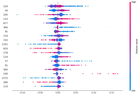
Figure 9.
SHAP summary plot for top 20 features from DDE + ESM2.
To further elucidate the impact of individual features on the model’s predictions, we analyzed the SHAP values for the top 20 features derived from the DDE + ESM2 feature combination, as depicted in Figure 9. This visualization provides insights into the direction and magnitude of each feature’s influence on the model’s output. Features with positive SHAP values contribute to a higher prediction score (FRPs), while features with negative SHAP values contribute to a lower prediction score (non-FRPs). The color intensity reflects the magnitude of the feature’s impact.
To gain further insights into the interactions between features, we generated a SHAP decision plot for the 216-dimensional feature set extracted from the combined DDE + ESM2 features. This plot illustrates the cumulative contribution of each feature to the model’s decision-making process, highlighting the most influential features and their interactions (Figure 10).
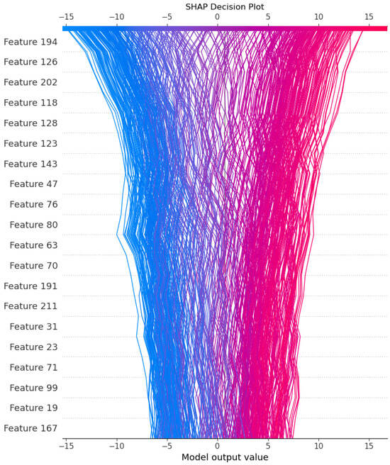
Figure 10.
SHAP decision plot for 216-dimensional feature set.
While SHAP analysis effectively quantifies individual feature contributions, directly mapping high-importance features from the combined DDE and ESM2 set to specific biological motifs presents inherent challenges. This difficulty arises from the abstract, high-dimensional nature of ESM2 embeddings, which capture complex, non-linear dependencies, and the statistical derivation of DDE features. Nevertheless, the significant contributions of these features strongly suggest that our model leverages underlying biological signals. For instance, the importance of DDE features indicates the model’s sensitivity to local amino acid environments, while the prominent role of ESM2 embeddings highlights the capture of global protein characteristics crucial for FRP prediction. This demonstrates that PLM-FRP effectively learns sophisticated biological patterns, even if they are not immediately interpretable as discrete biological units.
Through this comprehensive analysis, we have gained a deeper understanding of the model’s decision-making process, revealing the interplay among key features and their influence on FRP prediction. These insights not only enhance confidence in the model’s reliability but also contribute to a better understanding of the underlying biological factors associated with ferroptosis.
3.5. Web Server
To facilitate the widespread use of our model, we have developed a user-friendly web server, PLM-FRP, which is publicly accessible at https://www.frppredict.site (accessed on 6 July 2025). The server provides a convenient platform for researchers to submit protein sequences in FASTA format and obtain rapid predictions of their potential as FRPs.
The web server is built on the Flask framework, chosen for its lightweight nature and seamless integration with our Python-based machine learning pipeline. It is hosted on a cloud platform to ensure high availability, scalability, and efficient processing of user requests. Upon submission, the server processes the input sequences using our optimized PLM-FRP model. The results are promptly displayed, including a probability score indicating the likelihood of each sequence being an FRP. To enhance transparency and provide deeper insights, the server also presents the key underlying features (DDE and ESM2 embeddings) that contributed to the prediction.
Furthermore, to ensure the reproducibility and extensibility of our research, the complete source code for the training and prediction models, along with the datasets, is publicly available at our GitHub repository: https://github.com/Moeary/PLM_FRP (accessed on 2 June 2025). This repository includes all necessary scripts and detailed instructions, enabling other researchers to replicate our findings and build upon our work.
3.6. Discussion
3.6.1. Summary of Findings
The accurate identification of FRPs is crucial for advancing our understanding of ferroptosis and its role in various diseases. Our proposed method, PLM-FRP, leverages a multimodal approach by integrating traditional sequence-based features (DDE) with contextualized embeddings from the pre-trained protein language model ESM2. This hybrid feature set, refined through a robust LambdaRank-based feature selection strategy, enables PLM-FRP to capture a comprehensive range of biologically relevant information. Our results demonstrate that PLM-FRP achieves state-of-the-art performance, with a final accuracy of 96.09% on the independent test set, representing a significant improvement of approximately 4% over previous methods. This underscores the power of integrating diverse feature types, particularly the rich representations from PLMs, for complex biological prediction tasks.
3.6.2. Comparison with Deep Learning Models
Contrary to the common expectation that deep learning models like CNNs and BiLSTMs would yield superior performance, our XGBoost-based method consistently outperformed these architectures. Several factors may explain this observation. First, deep learning models typically require extensive datasets to learn complex patterns effectively, and our benchmark dataset, though well-curated, is of limited size. In such data-scarce scenarios, ensemble methods like XGBoost are often more robust and less prone to overfitting. Second, the strong performance of PLM-FRP is heavily reliant on its highly discriminative, engineered feature set (DDE + ESM2). While deep learning models can learn features end-to-end, the explicit provision of these potent, pre-extracted features to XGBoost proved more effective for this specific task. Finally, despite systematic hyperparameter optimization via grid search for the CNN and BiLSTM models, the inherent stability and powerful gradient boosting framework of XGBoost demonstrated superior performance with our optimized multimodal features.
3.6.3. Limitations and Future Directions
Despite its promising performance, PLM-FRP has several limitations that present opportunities for future research. The primary limitation is the relatively small size of the current benchmark dataset; expanding it with more diverse, experimentally validated FRPs would likely enhance the model’s generalizability. Additionally, while our negative dataset was carefully constructed, the evolving nature of biological discovery means some proteins currently labeled as non-FRPs might later be identified as having a role in ferroptosis, introducing potential label noise. Furthermore, the interpretability of the hybrid features, particularly the abstract embeddings from ESM2, remains a challenge. Future work should focus on developing advanced interpretation techniques to map these predictive features to concrete biological properties. Addressing these limitations by curating larger datasets and improving model interpretability will be crucial for developing the next generation of predictive tools for ferroptosis research.
4. Conclusions
In this study, we have introduced PLM-FRP, a novel machine learning framework designed for the accurate and efficient prediction of ferroptosis-related proteins (FRPs). Our approach successfully integrates traditional sequence-based features (DDE) with advanced contextual embeddings from the pre-trained protein language model ESM2. By employing a sophisticated feature selection strategy, we identified an optimal hybrid feature set that captures a comprehensive spectrum of biological information, from local amino acid composition to global evolutionary and structural properties.
The resulting model, PLM-FRP, achieves state-of-the-art performance, significantly outperforming existing methods on the independent test set. To enhance model transparency, we utilized SHAP analysis to interpret the contributions of individual features, providing valuable insights into the model’s decision-making process. Furthermore, we have developed a user-friendly web server to ensure broad accessibility, enabling researchers to leverage our powerful predictive tool with ease. PLM-FRP promises to be a valuable resource for accelerating the discovery of novel FRPs, deepening our understanding of ferroptosis mechanisms, and guiding the development of future therapeutic interventions. Future work will focus on expanding the training dataset and exploring more advanced deep learning architectures to further enhance predictive accuracy and interpretability.
Author Contributions
Conceptualization, J.Z. and C.W.; methodology, J.Z.; software, J.Z.; validation, J.Z.; formal analysis, J.Z.; investigation, J.Z.; resources, C.W.; data curation, J.Z.; writing—original draft preparation, J.Z.; writing—review and editing, C.W.; visualization, J.Z.; supervision, C.W.; project administration, C.W.; funding acquisition, C.W. All authors have read and agreed to the published version of the manuscript.
Funding
This research received no external funding.
Institutional Review Board Statement
Not applicable.
Informed Consent Statement
Not applicable.
Data Availability Statement
The source code and datasets generated for this study are publicly available in the GitHub repository: https://github.com/Moeary/PLM_FRP (accessed on 2 June 2025). Additional raw data or details can be obtained from the corresponding author upon reasonable request.
Acknowledgments
We thank the authors of the ESM-1b and ESM2 models for their pioneering work in protein language modeling, which has significantly advanced our understanding of protein sequences and their functional implications. And we also thank the authors of the MRMD3.0 tool for their valuable contributions to feature selection in protein prediction tasks.
Conflicts of Interest
The authors declare no conflicts of interest. The funders had no role in the design of the study; in the collection, analyses, or interpretation of data; in the writing of the manuscript; or in the decision to publish the results.
References
- Xie, Y.; Hou, W.; Song, X.; Yu, Y.; Huang, J.; Sun, X.; Kang, R.; Tang, D. Ferroptosis: Process and function. Cell Death Differ. 2016, 23, 369–379. [Google Scholar] [CrossRef] [PubMed]
- Bebber, C.M.; Müller, A. Ferroptosis in cancer cell biology. Cancers 2020, 12, 164. [Google Scholar] [CrossRef] [PubMed]
- David, S.; Jhelum, P.; Ryan, F.; Jeong, S.Y.; Kroner, A. Dysregulation of iron homeostasis in the central nervous system and the role of ferroptosis in neurodegenerative disorders. Antioxid. Redox Signal. 2022, 37, 150–170. [Google Scholar] [CrossRef] [PubMed]
- Li, X.; Ma, N.; Xu, J.; Zhang, Y.; Yang, P.; Su, X.; Xing, Y.; An, N.; Yang, F.; Zhang, G.; et al. Targeting ferroptosis: Pathological mechanism and treatment of ischemia-reperfusion injury. Oxidative Med. Cell. Longev. 2021, 2021, 1587922. [Google Scholar] [CrossRef] [PubMed]
- Dixon, S.J.; Lemberg, K.M.; Lamprecht, M.R.; Skouta, R.; Zaitsev, E.M.; Gleason, C.E.; Patel, D.N.; Bauer, A.J.; Cantley, A.M.; Yang, W.S.; et al. Ferroptosis: An iron-dependent form of nonapoptotic cell death. Cell 2012, 149, 1060–1072. [Google Scholar] [CrossRef] [PubMed]
- Hangauer, M.J.; Viswanathan, V.S.; Ryan, M.J.; Bole, D.; Eaton, J.K.; Matov, A.; Galeas, J.; Dhruv, H.D.; Berens, M.E.; Schreiber, S.L.; et al. Drug-tolerant persister cancer cells are vulnerable to GPX4 inhibition. Nature 2017, 551, 247–250. [Google Scholar] [CrossRef] [PubMed]
- Doll, S.; Proneth, B.; Tyurina, Y.Y.; Panzilius, E.; Kobayashi, S.; Ingold, I.; Irmler, M.; Beckers, J.; Aichler, M.; Walch, A.; et al. ACSL4 dictates ferroptosis sensitivity by shaping cellular lipid composition. Nat. Chem. Biol. 2017, 13, 91–98. [Google Scholar] [CrossRef] [PubMed]
- Park, E.; Chung, S.W. ROS-mediated autophagy increases intracellular iron levels and ferroptosis by ferritin and transferrin receptor regulation. Cell Death Dis. 2019, 10, 822. [Google Scholar] [CrossRef] [PubMed]
- Doll, S.; Freitas, F.P.; Shah, R.; Aldrovandi, M.; da Silva, M.C.; Ingold, I.; Goya Grocin, A.; Xavier da Silva, T.N.; Panzilius, E.; Scheel, C.H.; et al. FSP1 is a glutathione-independent ferroptosis suppressor. Nature 2019, 575, 693–698. [Google Scholar] [CrossRef] [PubMed]
- Lin, L.; Long, Y.; Liu, J.; Deng, D.; Yuan, Y.; Liu, L.; Tan, B.; Qi, H. FRP-XGBoost: Identification of ferroptosis-related proteins based on multi-view features. Int. J. Biol. Macromol. 2024, 262, 130180. [Google Scholar] [CrossRef] [PubMed]
- Lin, Z.; Akin, H.; Rao, R.; Hie, B.; Zhu, Z.; Lu, W.; Smetanin, N.; Verkuil, R.; Kabeli, O.; Shmueli, Y.; et al. Evolutionary-scale prediction of atomic-level protein structure with a language model. Science 2023, 379, 1123–1130. [Google Scholar] [CrossRef] [PubMed]
- Zagirova, D.; Pushkov, S.; Leung, G.H.D.; Liu, B.H.M.; Urban, A.; Sidorenko, D.; Kalashnikov, A.; Kozlova, E.; Naumov, V.; Pun, F.W.; et al. Biomedical generative pre-trained based transformer language model for age-related disease target discovery. Aging 2023, 15, 9293. [Google Scholar] [CrossRef] [PubMed]
- Zhou, N.; Yuan, X.; Du, Q.; Zhang, Z.; Shi, X.; Bao, J.; Ning, Y.; Peng, L. FerrDb V2: Update of the manually curated database of ferroptosis regulators and ferroptosis-disease associations. Nucleic Acids Res. 2022, 51, D571–D582. [Google Scholar] [CrossRef] [PubMed]
- Consortium, U. UniProt: The universal protein knowledgebase in 2023. Nucleic Acids Res. 2023, 51, D523–D531. [Google Scholar] [CrossRef] [PubMed]
- Roy, S.; Martinez, D.; Platero, H.; Lane, T.; Werner-Washburne, M. Exploiting amino acid composition for predicting protein-protein interactions. PLoS ONE 2009, 4, e7813. [Google Scholar] [CrossRef] [PubMed]
- Chen, Z.; Chen, Y.Z.; Wang, X.F.; Wang, C.; Yan, R.X.; Zhang, Z. Prediction of ubiquitination sites by using the composition of k-spaced amino acid pairs. PLoS ONE 2011, 6, e22930. [Google Scholar] [CrossRef] [PubMed]
- Nesmelova, I.V.; Hackett, P.B. DDE transposases: Structural similarity and diversity. Adv. Drug Deliv. Rev. 2010, 62, 1187–1195. [Google Scholar] [CrossRef] [PubMed]
- Liu, B.; Gao, X.; Zhang, H. BioSeq-Analysis2.0: An updated platform for analyzing DNA, RNA and protein sequences at sequence level and residue level based on machine learning approaches. Nucleic Acids Res. 2019, 47, e127. [Google Scholar] [CrossRef] [PubMed]
- Altschul, S.F.; Madden, T.L.; Schäffer, A.A. Gapped BLAST and PSI-BLAST: A new generation of protein database search programs. Nucleic Acids Res. 1997, 25, 3389–3402. [Google Scholar] [CrossRef] [PubMed]
- Wang, J.; Yang, B.; Revote, J.; Leier, A.; Marquez-Lago, T.T.; Webb, G.; Song, J.; Chou, K.C.; Lithgow, T. POSSUM: A bioinformatics toolkit for generating numerical sequence feature descriptors based on PSSM profiles. Bioinformatics 2017, 33, 2756–2758. [Google Scholar] [CrossRef] [PubMed]
- Su, C.T.; Chen, C.Y.; Ou, Y.Y. Protein disorder prediction by condensed PSSM considering propensity for order or disorder. BMC Bioinform. 2006, 7, 319. [Google Scholar] [CrossRef] [PubMed]
- Saini, H.; Raicar, G.; Lal, S.; Dehzangi, A.; Lyons, J.; Paliwal, K.K.; Imoto, S.; Miyano, S.; Sharma, A. Genetic algorithm for an optimized weighted voting scheme incorporating k-separated bigram transition probabilities to improve protein fold recognition. In Proceedings of the Asia-Pacific World Congress on Computer Science and Engineering, Nadi, Fiji, 4–5 November 2014; pp. 1–7. [Google Scholar]
- Vaswani, A.; Shazeer, N.; Parmar, N.; Uszkoreit, J.; Jones, L.; Gomez, A.N.; Kaiser, Ł.; Polosukhin, I. Attention is all you need. In Proceedings of the Advances in Neural Information Processing Systems 30 (NIPS 2017), Long Beach, CA, USA, 4–9 December 2017. [Google Scholar]
- Ferruz, N.; Schmidt, S.; Höcker, B. ProtGPT2 is a deep unsupervised language model for protein design. Nat. Commun. 2022, 13, 4348. [Google Scholar] [CrossRef] [PubMed]
- Rao, R.M.; Liu, J.; Verkuil, R.; Meier, J.; Canny, J.; Abbeel, P.; Sercu, T.; Rives, A. MSA Transformer; Cold Spring Harbor Laboratory: Cold Spring Harbor, NY, USA, 2021; pp. 8844–8856. [Google Scholar]
- Elnaggar, A.; Heinzinger, M.; Dallago, C.; Rehawi, G.; Wang, Y.; Jones, L.; Gibbs, T.; Feher, T.; Angerer, C.; Steinegger, M.; et al. ProtTrans: Towards Cracking the Language of Life’s Code Through Self-Supervised Deep Learning and High Performance Computing. bioRxiv 2020, 2020.07.12.199554. [Google Scholar] [CrossRef]
- Ofer, D.; Brandes, N.; Linial, M. The language of proteins: NLP, machine learning & protein sequences. Comput. Struct. Biotechnol. J. 2021, 19, 1750–1758. [Google Scholar] [CrossRef] [PubMed]
- Cui, F.; Zhang, Z.; Zou, Q. Sequence representation approaches for sequence-based protein prediction tasks that use deep learning. Briefings Funct. Genom. 2021, 20, 61–73. [Google Scholar] [CrossRef] [PubMed]
- He, S.; Ye, X.; Sakurai, T.; Zou, Q. MRMD3.0: A Python Tool and Webserver for Dimensionality Reduction and Data Visualization via an Ensemble Strategy. J. Mol. Biol. 2023, 435, 168116. [Google Scholar] [CrossRef] [PubMed]
- Liao, H.; Mariani, M.S.; Medo, M. Ranking in evolving complex networks. Phys. Rep. 2017, 689, 1–54. [Google Scholar] [CrossRef]
- Kohavi, R.; John, G.H. Wrappers for feature subset selection. Artif. Intell. 1997, 97, 273–324. [Google Scholar] [CrossRef]
- Burges, C.J. From ranknet to lambdarank to lambdamart: An overview. Learning 2010, 11, 81. [Google Scholar]
- Liu, H.; Yu, L. Toward integrating feature selection algorithms for classification and clustering. IEEE Trans. Knowl. Data Eng. 2005, 17, 491–502. [Google Scholar] [CrossRef]
- Drucker, H.; Wu, D.; Vapnik, V.N. Support vector machines for spam categorization. IEEE Trans. Neural Netw. 1999, 10, 1048–1054. [Google Scholar] [CrossRef] [PubMed]
- Breiman, L. Random forests. Mach. Learn. 2001, 45, 5–32. [Google Scholar] [CrossRef]
- Friedman, N.; Geiger, D.; Goldszmidt, M. Bayesian network classifiers. Mach. Learn. 1997, 29, 131–163. [Google Scholar] [CrossRef]
- LeCun, Y.; Bottou, L.; Bengio, Y.; Haffner, P. Gradient-based learning applied to document recognition. Proc. IEEE 1998, 86, 2278–2324. [Google Scholar] [CrossRef]
- Chen, T.; Guestrin, C. Xgboost: A scalable tree boosting system. In Proceedings of the 22nd Acm Sigkdd International Conference on Knowledge Discovery and Data Mining, San Francisco, CA, USA, 13–17 August 2016; pp. 785–794. [Google Scholar]
- Pedregosa, F.; Varoquaux, G.; Gramfort, A.; Michel, V.; Thirion, B.; Grisel, O.; Blondel, M.; Prettenhofer, P.; Weiss, R.; Dubourg, V.; et al. Scikit-learn: Machine learning in Python. J. Mach. Learn. Res. 2011, 12, 2825–2830. [Google Scholar]
- Wang, L.; Wang, H.F.; Liu, S.R.; Yan, X.; Song, K.J. Predicting protein-protein interactions from matrix-based protein sequence using convolution neural network and feature-selective rotation forest. Sci. Rep. 2019, 9, 9848. [Google Scholar] [CrossRef] [PubMed]
- Siami-Namini, S.; Tavakoli, N.; Namin, A.S. The performance of LSTM and BiLSTM in forecasting time series. In Proceedings of the International Conference on Intelligent Systems Design and Applications, Auburn, WA, USA, 3–5 December 2019; pp. 3285–3292. [Google Scholar]
- Zhao, R.; Yan, R.; Wang, J.; Mao, K. Learning to monitor machine health with convolutional bi-directional LSTM networks. Sensors 2017, 17, 273. [Google Scholar] [CrossRef] [PubMed]
- Syarif, I.; Prugel-Bennett, A.; Wills, G. SVM parameter optimization using grid search and genetic algorithm to improve classification performance. Telkomnika Telecommun. Comput. Electron. Control. 2016, 14, 1502–1509. [Google Scholar] [CrossRef]
- Elgeldawi, E.; Sayed, A.; Galal, A.R.; Zaki, A.M. Hyperparameter tuning for machine learning algorithms used for arabic sentiment analysis. Informatics 2021, 8, 79. [Google Scholar] [CrossRef]
- Wong, T.T.; Yeh, P.Y. Reliable accuracy estimates from k-fold cross validation. IEEE Trans. Knowl. Data Eng. 2019, 32, 1586–1594. [Google Scholar] [CrossRef]
- Lundberg, S. A unified approach to interpreting model predictions. arXiv 2017, arXiv:1705.07874. [Google Scholar] [CrossRef]
- Van der Maaten, L.; Hinton, G. Visualizing data using t-SNE. J. Mach. Learn. Res. 2008, 9, 2579–2605. [Google Scholar]
Disclaimer/Publisher’s Note: The statements, opinions and data contained in all publications are solely those of the individual author(s) and contributor(s) and not of MDPI and/or the editor(s). MDPI and/or the editor(s) disclaim responsibility for any injury to people or property resulting from any ideas, methods, instructions or products referred to in the content. |
© 2025 by the authors. Licensee MDPI, Basel, Switzerland. This article is an open access article distributed under the terms and conditions of the Creative Commons Attribution (CC BY) license (https://creativecommons.org/licenses/by/4.0/).