Article

Adaptive Nonlinear Proportional–Integral–Derivative Control of a Continuous Stirred Tank Reactor Process Using a Radial Basis Function Neural Network

by
Joo-Yeon Lee
1,
Gang-Gyoo Jin
2 and
Gun-Baek So
3,*
1
Ocean Space Development & Energy Research Department, Korea Institute of Ocean Science and Technology, Busan 49111, Republic of Korea
2
Department of Electrical Power and Control Engineering, Adama Science and Technology University, Adama 1888, Ethiopia
3
Department of Maritime Industry Convergence, Mokpo National Maritime University, Mokpo 58628, Republic of Korea
*
Author to whom correspondence should be addressed.
Algorithms 2025, 18(7), 442; https://doi.org/10.3390/a18070442
Submission received: 12 June 2025 / Revised: 6 July 2025 / Accepted: 14 July 2025 / Published: 18 July 2025

Abstract

Temperature control in a continuous stirred tank reactor (CSTR) poses significant challenges due to the process’s inherent nonlinearities and uncertain parameters. This study proposes an innovative solution by developing an adaptive nonlinear proportional–integral–derivative (NPID) controller. The nonlinear gain that dynamically scales the error fed to the integrator is enhanced for optimized performance. The network’s ability to approximate nonlinear functions and its online learning capabilities are leveraged by effectively integrating an NPID control scheme with a radial basis function neural network (RBFNN). This synergistic approach provides a more robust and reliable control strategy for CSTRs. To assess the proposed method’s feasibility, a set of simulations was conducted for tracking, disturbance rejection, and parameter variations. These results were compared with those of an adaptive RBFNN-based PID (APID) controller under identical conditions. The simulations indicated that the proposed method achieved reductions in maximum overshoot of 33.7% and settling time of 54.2% for upward and downward setpoint changes and 27.2% and 5.3% for downward and upward setpoint changes compared to the APID controller. For disturbance changes, the proposed method reduced the peak magnitude (Mpeak) by 4.9%, recovery time (trcy) by 23.6%, and integral absolute error by 16.2%. Similarly, for parameter changes, the reductions were 3.0% (Mpeak), 26.4% (trcy), and 24.4% (IAE).

1. Introduction

Continuous stirred tank reactors (CSTRs) are widely used in industrial chemical processes. These reactors maintain constant mixing, ensuring uniform reactant distribution and product removal. However, exothermic reactions within CSTRs can generate substantial heat, potentially leading to uncontrolled reactions and safety hazards. To prevent thermal runaway and overheating, effective temperature control through cooling mechanisms is essential for stabilizing the reaction process.
Extensive research has been conducted on temperature control in CSTR processes, exploring various controller structures and tuning methods [1,2]. While traditional fixed-gain proportional–integral–derivative (PID) controllers offer simplicity and cost-effectiveness [3,4], their performance can deteriorate when operating conditions deviate from the design point or when applied to highly nonlinear systems like CSTRs. This limitation has driven the development of advanced PID controller variants [5]. Several approaches aim to address the nonlinearities inherent in control systems. These include gain scheduling, fractional-order techniques, and nonlinear PID control structures. Gain scheduling techniques enhance control performance by adjusting controller gains according to the system’s current operating conditions, effectively linearizing the system around various operating points. Ranjan and Chakraborty [6] presented a gain-scheduled composite nonlinear feedback controller for CSTRs, combining linear and nonlinear control laws. Bingi et al. [7] conducted a comparative study of 2-DOF (2-degree-of-freedom) PID and 2DOF fractional-order PID (FOPID) controllers, reviewing their different forms. Poovarasan et al. [8] successfully applied a fractional-order PID controller to regulate CSTR process parameters within desired limits. The FOPID controller parameters were optimized using genetic algorithms and particle swarm optimization. Building upon these advancements, Wase et al. [9] integrated the strengths of both fractional-order PID control and fuzzy logic. This hybrid approach utilizes fractional-order PID controllers as local controllers within distinct operating regions, enhancing control performance. A Takagi-Sugeno fuzzy gain scheduling mechanism then seamlessly transitions between the outputs of these local controllers, ensuring smooth and adaptive control across the entire operating range.
Nonlinear proportional–integral–derivative (NPID) control strategies have been extensively investigated for systems exhibiting complex and time-varying dynamics, building upon Seraji’s pioneering research [10,11]. NPID controllers offer significant advantages by allowing for customization through the adjustment of their nonlinear functions and parameters. This flexibility enables precise tuning of the control system to achieve optimal performance. Contributing to the several notable advancements in NPID control, Seraji [10,11] pioneered a novel approach to nonlinear PID control. He introduced a class of controllers that incorporate a nonlinear gain element in cascade with a conventional linear fixed-gain PID controller. This framework explored three distinct nonlinear gain functions: the sigmoidal function, the hyperbolic function, and the piecewise-linear function. The stability of the closed-loop systems resulting from these configurations was rigorously analyzed using the Popov stability criterion. To improve the control performance, Aydogdu and Korkmaz [12] developed a dynamic NPID controller that adapts its parameters in real time based on the system’s error. Li et al. [13] proposed an NPID controller that effectively combines linear and nonlinear elements, particularly by adjusting the integral gain using a Gaussian function. So and Jin [14] introduced a design method for a nonlinear variable-gain PID controller, where the gains are determined by a set of fuzzy rules. The optimal parameter values for this controller were determined using a genetic algorithm. While offering enhanced performance, designing and tuning NPID controllers can often be more complex than their linear counterparts. A novel NPID controller that addresses this challenge was presented in [15,16]. By scaling the error input to the integrator within the standard PID controller framework, the number of tuning parameters is maintained at three, simplifying the design and tuning process.
To further improve control precision and stability, researchers have increasingly incorporated advanced control strategies including adaptive control and intelligent techniques like evolutionary algorithms, neural networks, and fuzzy logic. In [17], the authors investigated the design and performance of internal model control and model reference adaptive control (MRAC) for the linearized second-order model of a CSTR process. In [18], the authors explored an improved method for controlling the temperature of a continuous reactor; an improved Sparrow Algorithm was used to find the best settings of a PID controller. In [19], the authors proposed the use of a neuro-fuzzy control system, optimized by a metaheuristic technique, for precise temperature control in a chemical reactor during biodiesel production. In [20], the authors developed a type of adaptive controller for systems in which a linear part is followed by a nonlinear part. This controller uses both linear and nonlinear control methods to achieve better performance. This paper presents a fuzzy adaptive control scheme for continuous stirred tank reactors (CSTRs) subject to full-state constraints and actuator faults. Employing backstepping design in conjunction with an Integral Barrier Lyapunov Function (IBLF), the control strategy effectively addresses the limitations imposed by the full-state constraints. Anbu and Jaya [21] presented the design of a Model Reference Adaptive System (MRAS) utilizing the MIT rule. The MIT rule, employing a gradient-based method, adjusts the controller gain to minimize the discrepancy between the actual plant’s behavior and the desired behavior defined by a reference model. In [22], the authors studied an adaptive neural network (NN) control strategy for CSTRs operating under the influence of time-varying delays and subject to full time-varying state constraints. The time-delayed terms are decomposed into a sum of positive continuous functions using a separation technique. Subsequently, Lyapunov–Krasovskii functionals are employed to effectively address the stability concerns arising from these positive continuous functions containing delayed states. In [23], the authors proposed two neural network (NN)-based adaptive control strategies for continuous stirred tank reactors (CSTRs) subject to input nonlinearities and unknown disturbances. The first approach incorporates a robust control term to mitigate the impact of input dead zones. The second approach utilizes an anti-windup compensator to alleviate the effects of actuator saturation. Shi et al. [24] proposed an RBF-NPID control algorithm to improve the adaptive capability of the NPID controller for CSTRs. The RBF neural network is used to adjust nonlinear gains online to improve the control performance of the system. A characteristic of this approach is the adaptation of three nonlinear PID gains, which necessitates defining nine constants. Li et al. [25] presented a novel adaptive fuzzy control scheme for CSTRs that effectively addresses full-state constraints and actuator faults. The proposed controller utilizes IBLF to ensure that all state variables remain within their specified bounds. The adaptive fuzzy control mechanism is designed to compensate for uncertainties in the system dynamics. In [26], the authors proposed an approach that combined sliding mode control with an event-triggering mechanism to ensure stability and disturbance rejection under limited network resources. Chaturvedi et al. [27] introduced a neural network-based PID controller for CSTR temperature regulation. The neural network’s output layer weights—corresponding to proportional, integral, and derivative gains—were tuned using Particle Swarm Optimization (PSO). In [28], the authors developed a computational intelligence-based controller for CSTR concentration control, employing a radial basis function neural network (RBFNN) optimized via hybrid PSO variants. These advanced control schemes have offered distinct advantages but also have limitations, leaving room for improvement [29,30].
Building on the existing literature, this study introduces an adaptive NPID control scheme that enhances the robustness and reliability of CSTR control. The strengths of NPID control (customizable nonlinear functions and parameters) are synergistically combined with the function approximation and online learning capabilities of RBFNNs, retaining the benefits of the conventional PID controller, including its simple structure and three tuning parameters. To prevent excessive integral action, the error input to the integral action of the NPID controller is scaled by a nonlinear function—specifically, the product of the error and a nonlinear gain. The proposed method’s effectiveness is rigorously evaluated through simulations encompassing tracking performance, disturbance rejection, and parameter variations. The key contributions of this study are as follows:
  • To propose a nonlinear adaptive PID control technique combining the existing nonlinear PID controller and an RBFNN;
  • To refine the NPID controller’s gain function to enhance its performance.
This paper is organized as follows: Section 1 contains the introduction. Section 2 presents the modeling of a CSTR and its identification using the RBFNN. In Section 3, an adaptive control strategy is provided based on the identified model and an NPID controller. In Section 4, a set of simulations are conducted to observe the performance of the proposed method. Finally, the conclusion is presented in Section 5.

2. Problem Statement

2.1. CSTR Process Modeling

A continuous stirred tank reactor (CSTR) serves as a well-mixed vessel in industrial processes, with reactants continuously entering and products continuously exiting. Continuous stirring ensures uniform mixing and a consistent reaction rate. Figure 1 depicts a schematic diagram of the CSTR.
In Figure 1, CAf and Tf represent the reactant concentration and reactor temperature at the inlet of the reactant, respectively. CA and T denote the corresponding values at the outlet. F is the reactant flow rate. Similarly, Tcf and Tc represent the coolant temperature at the inlet and outlet, respectively. Fc is the coolant flow rate.
CSTRs are known for their challenging control due to highly nonlinear and complex behavior. This study investigates a CSTR where an exothermic, first-order reaction (A→B) takes place. Maintaining a constant internal temperature is critical for achieving optimal reaction conditions within the reactor. Assuming thorough stirring, a constant volume, identical input and output flow rates, and constant physical parameters, the following equations can be derived by applying the principles of mass and energy conservation in the reactor and jacket [31,32,33]:
Reactant   material   balance :   d C A d τ = F V ( C A f C A ) k 0 exp ( E R T ) C A ,
Energy   balance   in   the   reactor :   d T d τ = F V ( T f T ) Δ H k 0 C A ρ C p exp ( E R T ) + U A ρ C p V ( T c T ) ,
Energy   balance   in   the   jacket :   d T c d τ = F c V j ( T c f T c ) U A ρ j C p j V j ( T c T ) ,
The parameters are listed in Table 1.
In general, the jacket temperature dynamics respond swiftly to changes in the reactor’s state. This implies that the time constant of the jacket temperature dynamics is much shorter than that of the reactor. Given this fact, the jacket’s dynamics can be neglected. Then, a simple steady-state equation can easily be obtained between the coolant flow rate Fc and the coolant temperature Tc:
T c = ρ j C p j F c T c f + U A T ρ j C p j F c + U A .
The primary control objective for the CSTR process is to maintain a stable reactor temperature (T) at a desired setpoint. To achieve this, the coolant flow rate is manipulated. However, due to the inherent relationship between Fc and Tc as defined in (2), utilizing Tc as the control input can simplify controller synthesis. Following the approach of previous studies [1,31,32,33], the coolant jacket temperature Tc is employed as the control input in this work. Then, Equation (1) becomes a dynamic equation governed by two variables CA and T exclusively. To express them more succinctly, the dimensionless variables and parameters are introduced as
γ = E R T f ,   H = Δ H C A f γ C p T f ,   β = U A F C p   and   D a = V k 0 e γ F ,
x 1 = C f C A C f ,   x 2 = T T f T f γ ,   u = T c T f T f γ   a n d   t = τ F V ,
where γ is the dimensionless activation energy, H is the dimensionless heat of the reaction, β is the dimensionless cooling rate, and Da is the Damköhler number. x1, x2, u, and t are the dimensionless reactant concentration, reactor temperature, jacket coolant temperature, and time, respectively. Then, the state space form considering external disturbances becomes as follows [30,31]:
x ˙ 1 ( t ) = x 1 ( t ) + D a [ 1 x 1 ( t ) ] exp [ x 2 ( t ) 1 + x 2 ( t ) / γ ] + d 1 ( t ) ,
x ˙ 2 ( t ) = ( 1 + β ) x 2 ( t ) + H D a [ 1 x 1 ( t ) ] exp [ x 2 ( t ) 1 + x 2 ( t ) / γ ] + β u ( t ) + d 2 ( t ) ,
y ( t ) = x 2 ( t ) .
where u represents the control input, y denotes the output temperature, and d1 and d2 denote disturbances in the reactant concentration and feed temperature, respectively.

2.2. Process Analysis

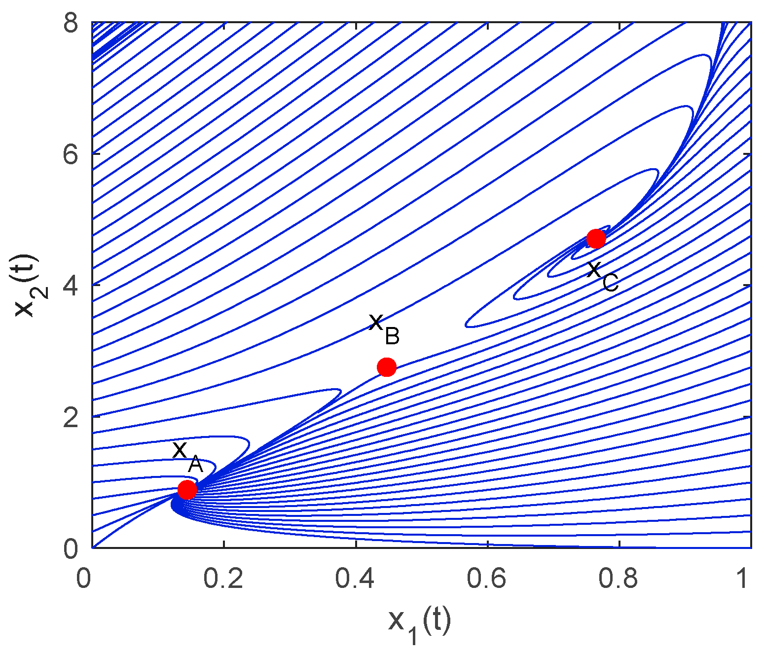
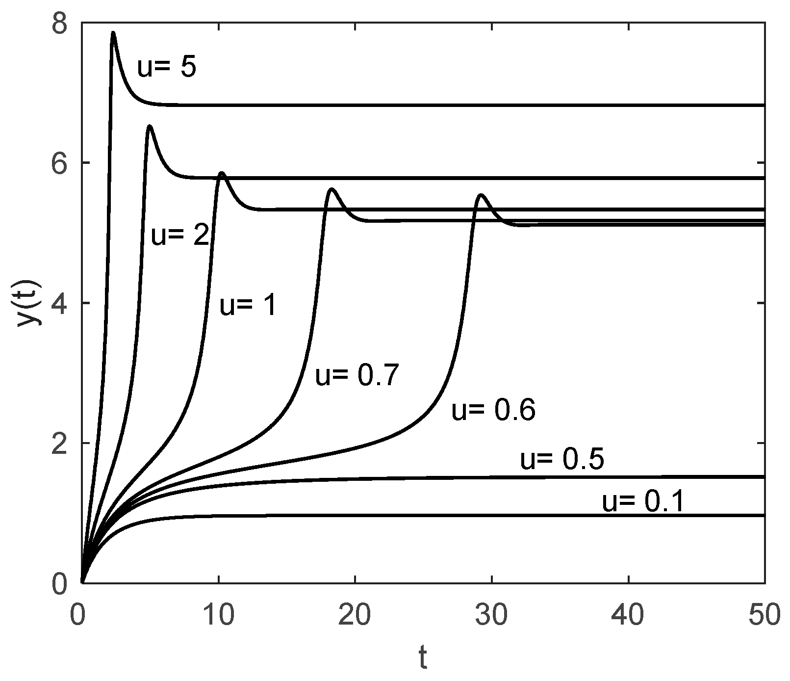
Two types of process analyses are considered here: equilibrium and dynamic. Equilibrium state analysis examines the steady-state conditions where all system variables remain constant over time. For this analysis, the input (u) is assumed to be zero, and all-time derivatives within the set of ordinary differential equations (ODEs) (4) are considered to be zero. This simplification transforms the ODEs into a set of nonlinear static equations which can then be solved analytically. Given the nominal parameter values Da = 0.072, γ = 20, H = 8, and β = 0.3, the process exhibits three equilibrium states (or points): xA = [0.144, 0.886]T, xB = [0.447, 2.752]T, and xC = [0.765, 4.705]T. These equilibria are characterized by complex dynamic behavior. While xA and xC are stable equilibria, xB is unstable. Figure 2 illustrates these equilibria on a phase diagram. Dynamic analysis investigates the process’s behavior in response to an abrupt input change. Figure 3 depicts the output response of the CSTR to step changes in the control input (u), demonstrating a clear dependence of response speed and steady-state gain on the magnitude of u. These nonlinear characteristics of the CSTR may hinder the effectiveness of a conventional PID controller with fixed gains across its entire operating range.

2.3. RBFNN-Based Process Identification

To overcome the drawbacks of conventional PID controllers in controlling CSTRs, an adaptive nonlinear PID (NPID) control strategy is proposed. This approach utilizes a more accurate CSTR model, implemented through a radial basis function neural network (RBFNN). The RBFNN provides online estimates of the output’s sensitivity to control inputs, allowing for dynamic adjustments of the NPID controller’s gains. System identification using an RBFNN involves developing a network model that accurately reflects the behavior of the CSTR based on observed I/O data. The following series-parallel model is adopted for identification:
y ( k + 1 ) = f ( y ( k ) , , y ( k n y ) , u ( k ) , u ( k n u ) ) ,
where f: ℜn → ℜ is a nonlinear function, y and u are the output and input of the process, respectively, nu and ny are the number of past input and past output samples required for model prediction, and k is the discrete time instance.
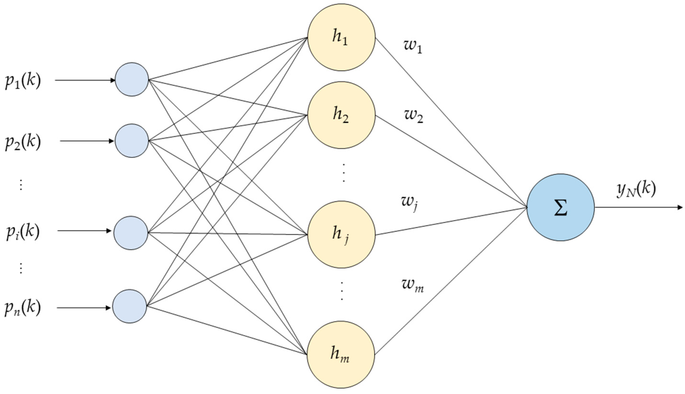
RBFNNs are well known for their robustness to nonlinearities, making them suitable for this application. RBFNNs with a two-layer architecture, a specialized type of neural networks (NN), are well suited for tasks like function approximation and time-series forecasting, offering fast training and universal approximation capabilities [34,35]. The input layer receives data and passes it to the hidden layer, which employs radial basis functions (RBFs) as activation functions. Each RBF neuron is characterized by a center and a width. The output layer generates the final output. RBFNNs are trained efficiently in two stages, outperforming traditional backpropagation networks in terms of speed. They possess the ability to approximate any continuous function to any desired level of accuracy and are adept at interpolating data points effectively. The theoretical foundation of RBFNNs supports their capacity to approximate any continuous function with arbitrary precision. Figure 4 shows the structure of an RBFNN, which comprises three layers.
When an input vector p = [p1, p2, …, pn]T ∈ ℜn is applied at the input side, each RBF in the hidden layer is activated. Let the RBF vector be h = [h1, h2, …, hj, …, hm]T ∈ ℜm, where hj is a Gaussian function given by
h j = exp [ ( p c j ) T ( p c j ) 2 b j 2 ]   ( j = 1 , 2 , , m ) ,
where n is the number of inputs and m is the number of neurons. The center vector at node j is cj = [cj1, cj2, …, cjn]T ∈ ℜn and the width bj (> 0) is the radial parameter of node j. Assuming that the weight vector of the network is W = [w1, w2, …, wm]T ∈ ℜm, the network output is calculated by
y N ( k ) = W T h = j = 1 m w j exp [ ( p c j ) T ( p c j ) 2 b j 2 ] .
A performance index criterion is defined for the given RBFNN during a training epoch as
E ( k ) = 1 2 [ y ( k ) y N ( k ) ] 2 ,
where y(k) is the desired output of the process and yN(k) is the network output. The input is fed into the RBFNN model. The network’s output is then compared to the actual system’s output, and the difference between the two is calculated. Then, the weight, center, and width of the RBFNN are updated as follows:

2.3.1. Weight Update

Employing gradient descent as the learning rule, the weight parameters of the RBFNN defined by (7) are iteratively updated to minimize the network’s error as
w j ( k ) = w j ( k 1 ) η w E w j ,
where ηw denotes the learning rate. By applying the chain rule, the gradient in (9) can be further expanded as
E w j = E y N × y N w j = [ y ( k ) y N ( k ) ] h j .
Substituting (10) into (9) and then including the momentum term, the update of the weights is given by
w j ( k ) = w j ( k 1 ) + Δ w j ( k ) + α [ w j ( k 1 ) w j ( k 2 ) ] ,
Δ w j ( k ) = η w E w j = η w [ y ( k ) y N ( k ) ] h j ,
where α is the momentum factor.

2.3.2. Center Update

By applying gradient descent, the online update of the centers is given by
c j i ( k ) = c j i ( k 1 ) η c E c j i ,
where ηc denotes the learning rate. The gradient in (13) can be further expanded as
E c j i = E y N × y N c j i = [ y ( k ) y N ( k ) ] y N c j i .
The gradient in (14) can be further expanded as
y N c j i = y N h j × h j c j i = w j h j ( x i c j i ) b j 2 .
Substituting (13) and (14) into (12) and incorporating the momentum term, the following is obtained:
c j i ( k ) = c j i ( k 1 ) + Δ c j i ( k ) + α [ c j i ( k 1 ) c j i ( k 2 ) ]
Δ c j i ( k ) = η c E c j i = η c [ y ( k ) y N ( k ) ] w j h j x i c j i b j 2

2.3.3. Width Update

Similar to the previous method, the update equation for the widths can be obtained as
b j ( k ) = b j ( k 1 ) η h E b j ,
where ηh is the learning rate. Applying the chain rule to the gradient in (16) yields the following equations:
b j ( k ) = b j ( k 1 ) + Δ b j ( k ) + α [ b j ( k 1 ) b j ( k 2 ) ]
Δ b j ( k ) = η h E b j = η h [ y ( k ) y N ( k ) ] w j h j | | x c j | | 2 b j 3
Following online system identification, the gains of the proposed controller are updated using the Jacobian matrix.

3. Design of Adaptive Nonlinear PID Controller

While fixed-parameter PID controllers generally exhibit good response characteristics within their designed operating range, their effectiveness may degrade and even lead to instability when the operating range deviates from the expected range. To address these limitations, various nonlinear PID (NPID) control strategies have been developed [10,11,12,13,14,15].

3.1. Existing PID Controllers

In this section, the standard linear controller and the nonlinear PID controller are considered and applied to adaptive control studies.

3.1.1. Linear PID Controller

Linear PID controllers are commonly employed in industrial control loops. They are a versatile tool that finds applications in various fields. The time domain equation is given by
u ( t ) = K p e ( t ) + K i e ( t ) d t + K d d e ( t ) d t ,
where e(t) is the error between a desired temperature and the process output temperature, and Kp, Ki, and Kd are the proportional, integral, and derivative gains, respectively. The PID controller functions by continuously assessing the difference between the desired output (setpoint) and the actual output. This error signal is then used to adjust the control input, aiming to minimize the error and stabilize the system around the setpoint.

3.1.2. Nonlinear PID Controller

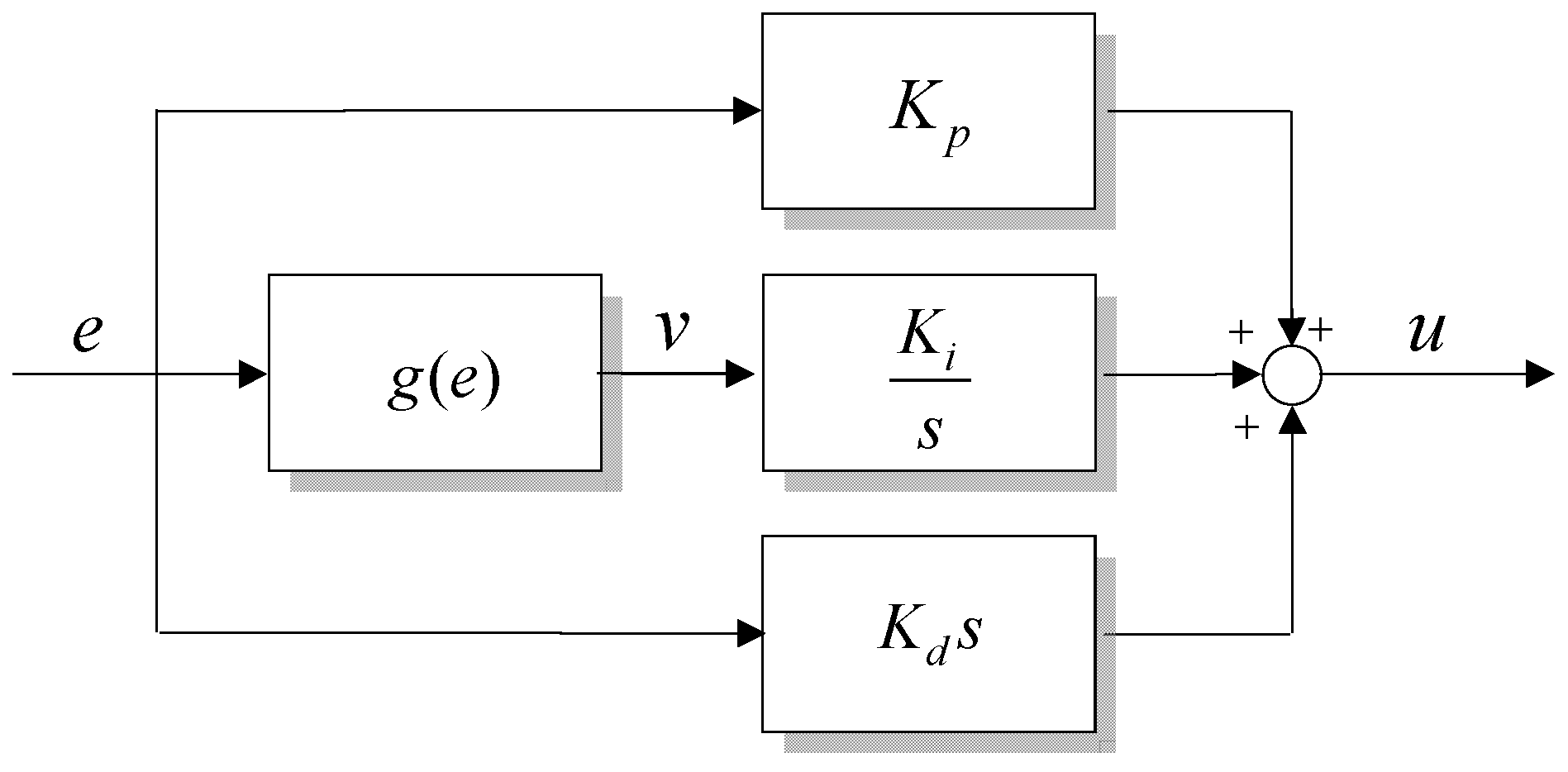
For nonlinear processes, NPID controllers offer advantages, such as smoother operation and improved resilience to unforeseen disturbances. NPID controllers are more complex to design and implement than linear PID controllers due to their increased number of tuning parameters. To address this, the author proposed a novel NPID controller, an enhancement over the conventional PID framework. This NPID controller requires only three tuning parameters [15]. To mitigate the limitations of traditional PID controllers, specifically the integral action’s susceptibility to overshoot, oscillations, and integral windup during dynamic conditions, the NPID controller incorporates a nonlinear gain. This nonlinear gain dynamically adjusts the error signal fed to the integrator, resulting in improved controller performance during sudden setpoint changes and disturbances. The time domain equation of this controller is described by
u t = K p e t + K i v t d t + K d d e ( t ) d t ,
where the error e(t) and gains Kp, Ki, and Kd are consistent with those of the previous PID controller. Meanwhile, v(t) is the scaled error given by
v ( t ) = g ( e ) e ( t ) ,
where g(e) is a nonlinear gain function of e represented by
g ( e ) = exp ( e 2 2 Δ r 2 ) .
Δr, a constant, represents the upper bound of the magnitude of setpoint changes between steps. Figure 5 depicts the structure of the NPID controller.

3.2. Enhanced Nonlinear PID Controller

The integral action of the above NPID controller nonlinearly scales down the error signal. This minimizes the offset for small errors and prevents excessive accumulation and overshoot for large errors. In this work, the integral action uses an enhanced nonlinear function as follows:
g ( e ) = a exp ( e 2 2 Δ r 2 ) ,
where a is a constant that determines the shape of g(e). This nonlinear gain slightly increases the error to reduce the offset by increasing the accumulated error when the error is small. Substituting (22) into (20) yields
v ( t ) = a e ( t ) exp ( e 2 2 Δ r 2 ) .
The constant a is chosen such that the function ν(t) converges to the value of e when e equals Δr. Applying this condition to (23), the following relationship is obtained:
a = exp ( 1 2 ) .
Substituting (24) into (23) gives the nonlinear gain function as
g ( e ) = exp ( 1 2 e 2 2 Δ r 2 ) .
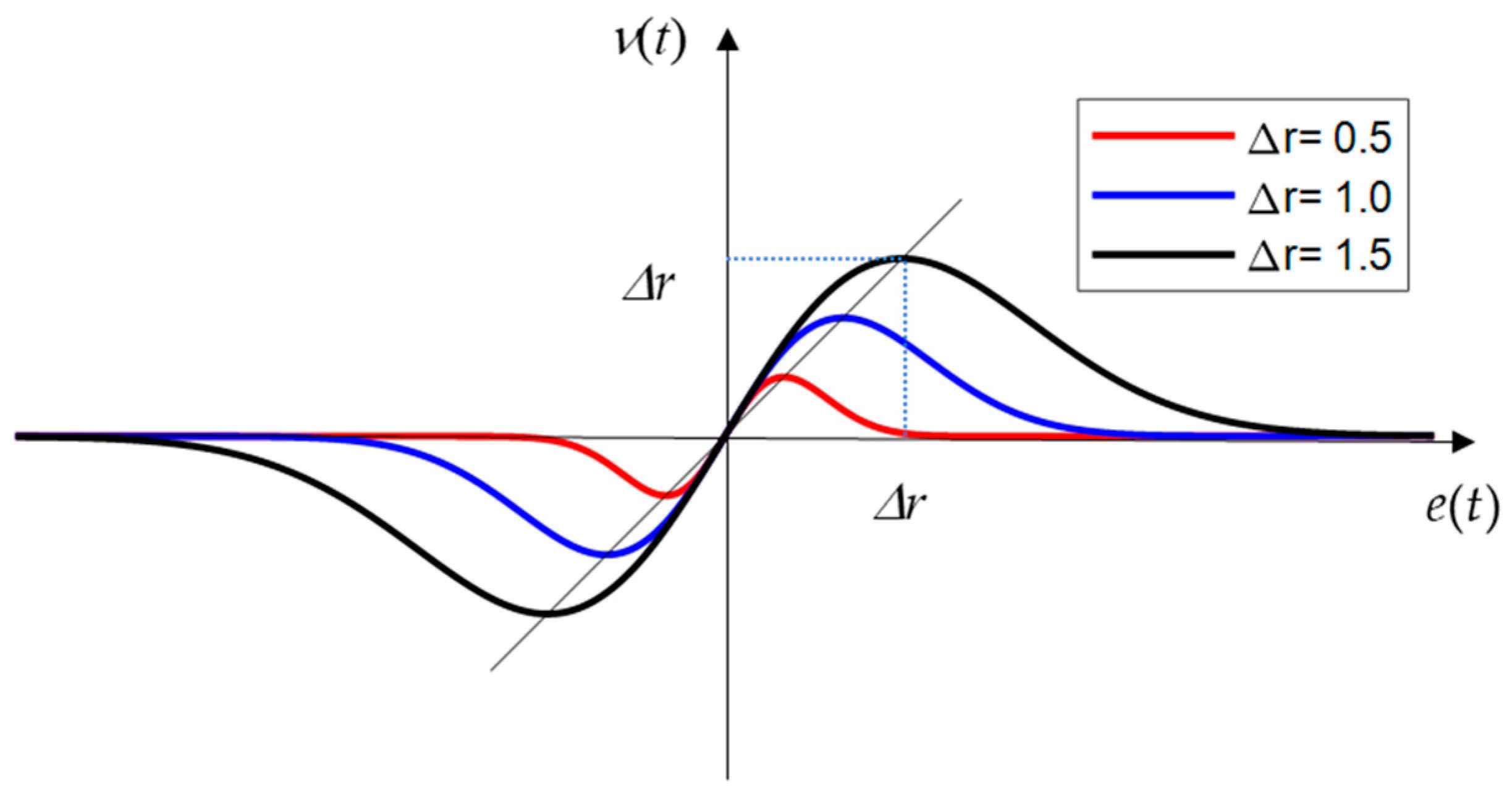
Figure 6 shows the scaled error ν(t) for different Δr values.
The integral action of the standard PID controller uses e(t) as is, but as seen in Figure 6, the new g(e) allows minor errors to be slightly amplified, thereby diminishing the steady-state error, and conversely, significant errors are abruptly scaled down to prevent excessive overshoot caused by the accumulated error.
To evaluate the tracking and disturbance rejection capabilities of the standard PID and NPID controllers, their performance is analyzed on a first-order plus time delay (FOPTD) system as
T d y ( t ) d t + y ( t ) = K u ( t L ) ,
where T is the time constant, K is the steady-state gain, and L is the time delay. Adjusting a controller’s settings impacts both its responsiveness to the desired setpoint and its ability to manage disturbances. These two settings often conflict. This trade-off is explored by simulating an FOPTD system with K = 1 and a dimensionless ratio (L/T).
To evaluate a controller’s performance, the following integral absolute error (IAE) performance criteria are used:
I A E S P = 0 | y r ( t ) y ( t ) | d t ,
I A E D I S = 0 | y ( t ) | d t ,
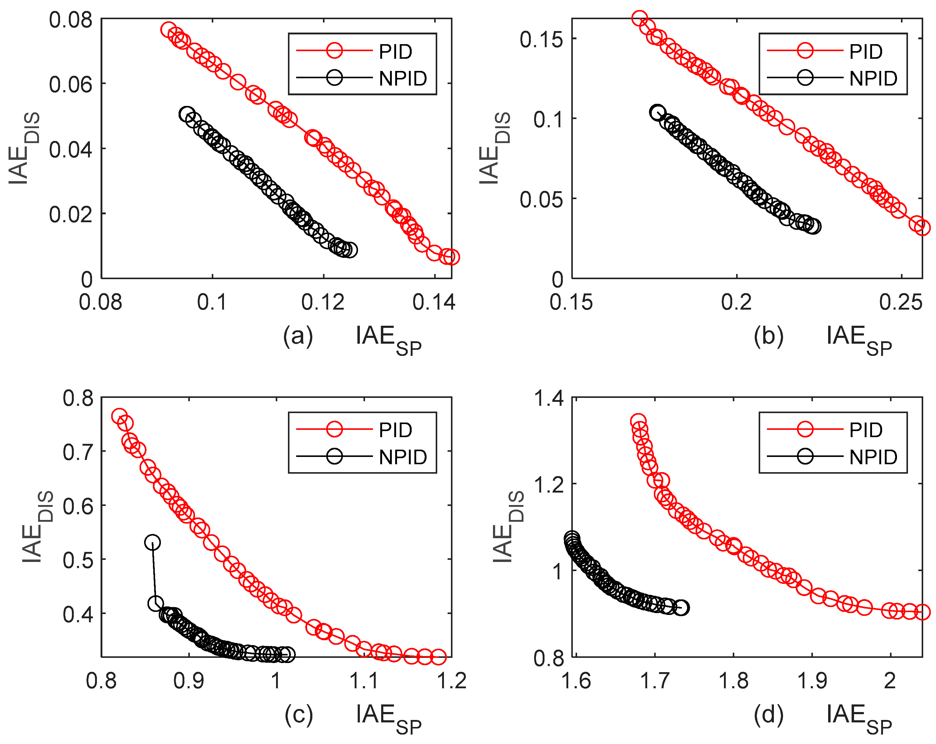
where IAESP is a measure of the error between the setpoint and the output over time while applying yr = 1 and d = 0, and IAEDIS the same measure while applying yr = 0 and d = 1. The disturbance d is considered to be added to the input side. A non-dominated sorting genetic algorithm (NSGA-II) [36,37] is applied to minimize the two performance metrics simultaneously for four distinct ratios of L/T: 0.01, 0.1, 0.5 and 1. Figure 7 shows the optimal Pareto fronts.
Figure 7 illustrates the fundamental trade-off between achieving good setpoint tracking and strong disturbance rejection. Enhancing one performance metric often necessitates compromising on the other. Our analysis reveals that the NPID controller outperforms the linear PID controller in this regard.

3.3. Proposed Adaptive NPID Controller

This subsection presents an adaptive NPID control scheme, where the three gains in (19) are adjusted adaptively. Assuming that the sampling time is small, the discrete time equation for the NPID controller is expressed by the following formula:
u ( k ) = K p e ( k ) + K i Δ t j = 0 k v ( j ) + K d e ( k ) e ( k 1 ) Δ t ,
where Δt is the sampling time, t = k·Δt, and e(k) is the error defined as
e k = y r k y k .
In (30), yr(k) is the desired temperature and y(k) is the measured output temperature. We rearrange the discrete time formula as follows:
u ( k ) = K p u 1 ( k ) + K i u 2 ( k ) + K d u 3 ( k ) .
where the three input components are as follows:
u 1 ( k ) = e ( k ) ,
u 2 ( k ) = Δ t j = 0 k v ( j ) ,
u 3 ( k ) = e ( k ) e ( k 1 ) Δ t .
The RBFNN then adjusts the controller gains to minimize the following performance index:
J = 1 2 e 2 ( k )
By adopting the gradient method, the updating equations for the NPID controller gains are
Δ K p ( k ) = η p J K p = η p J y y u u K p = η p e ( k ) y u u 1 ( k ) ,
Δ K i ( k ) = η i J K i = η i J y y u u K i = η i e ( k ) y u u 2 ( k ) ,
Δ K d ( k ) = η d J K d = η d J y y u u K d = η d e ( k ) y u u 3 ( k ) ,
where ηp, ηi, and ηd are the rates of change for the proportional, integral, and derivative gains, respectively, and y / u denotes the Jacobian matrix, which measures the sensitivity of the output to changes in the control input. As time progresses, the RBFNN identifier resembles the CSTR process, so y / u is calculated using the RBFNN presented in Section 2 as
y u y N u = u j = 1 m w j h j = j = 1 m w j h j c i 1 p 1 b j 2 ,
where p1 is the first element of the network input vector, so p1 = u(k).
Finally, the adaptation algorithm adjusts the three gains of the NPID controller as follows:
K p ( k ) = K p ( k 1 ) + Δ K p ( k )
K i ( k ) = K i ( k 1 ) + Δ K i ( k )
K d ( k ) = K d ( k 1 ) + Δ K d ( k )
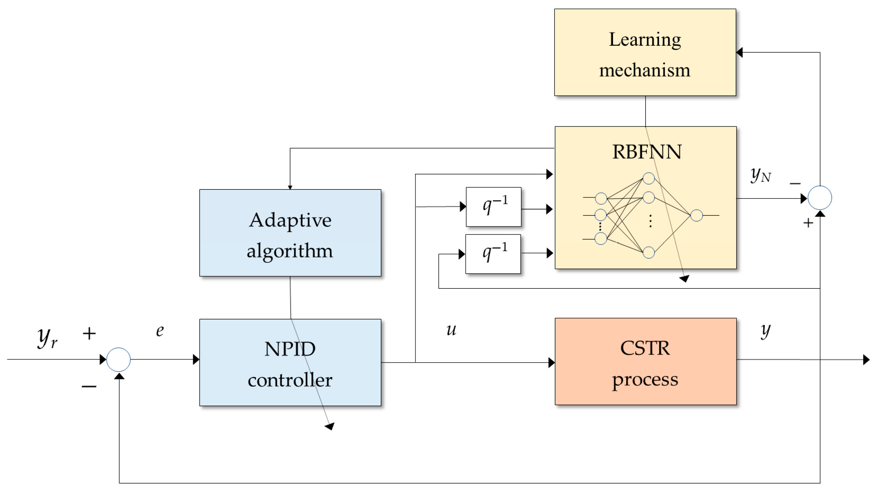
Figure 8 shows the proposed adaptive NPID control scheme based on the RBFNN, where q−1 denotes the delay operator.
The pseudocode representation of the proposed adaptive NPID controller, incorporating an RBFNN, is as Algorithm 1:
Algorithm 1 The pseudocode representation with RBFNN
Step 1: Initialize the adaptive NPID controller gains and RBFNN parameters and set other necessary parameters;
Step 2: Set time k = 0;
While <Termination condition is not met> do Steps 3–9
    Step 3: Update the NPID controller gains using (34)–(40);
    Step 4: Calculate the NPID control input using (19)–(20) and (25);
    Step 5: Numerically integrate the CSTR model in (4) to obtain y(k) at the kth instant;
    Step 6: Calculate the output of the RBFNN using (7) and update its weights, centers and widths using (11), (15) and (17);
    Step 7: Calculate the Jacobian matrix y / u using (37);
    Step 8: Update time k = k + 1;
    Step 9: Output y(k);
end

4. Simulation Results

This section evaluates the performance of the proposed adaptive NPID controller (hereafter referred to as ANPID) in terms of setpoint tracking, disturbance rejection, and robustness to parameter variations. The performance of the ANPID is assessed using the model defined in (4) and MATLAB 2018a software, and compared to that of an adaptive PID controller (hereafter referred to as APID). The weights, centers, and widths of the RBFNN for both controllers are subsequently updated based on the algorithms derived in the preceding section for a fair comparison. Setpoint tracking performance is evaluated based on overshoot (Mp), rise time (tr), 5% settling time (ts), and the integral of absolute error (IAE), which is assessed as follows:
I A E = 0 | e ( t ) | d t
For disturbance rejection, parameter variations, the perturbation peak (Mpeak), recovery time (trcy), and IAE, Mpeak denotes the maximum absolute deviation from the setpoint, while trcy signifies the time required to return within 2% of the setpoint following a disturbance.

4.1. Process and Control System Configurations

The dimensionless CSTR model was simulated with nominal parameter values of Da = 0.072, γ = 20, H = 8, and β = 0.3. This study utilized a 3-20-1 RBFNN architecture: 3 inputs, 20 hidden neurons, and 1 output. The network inputs are the current input (u(k)), the previous input (u(k − 1)), and the previous output (y(k − 1)), represented as the input vector p = [u(k), u(k − 1), y(k − 1)]T. The RBFNN identifier was trained online using a learning rate (ηw, ηc, ηh) of 0.05 and a momentum factor (α) of 0.01. The initial centers and widths of the RBFNN were randomly selected within the ranges [−15, 15] and [0, 20], respectively. The ANPID and APID controllers were configured with learning rates of 0.08, 0.03, and 0.02 for proportional, integral, and derivative gains, respectively. Both controllers began with the same initial gains of Kp = 0.5, Ki = 1, and Kd = 0.2, obtained through trial and error, to provide a challenging starting point.

4.2. Setpoint Tracking Performance

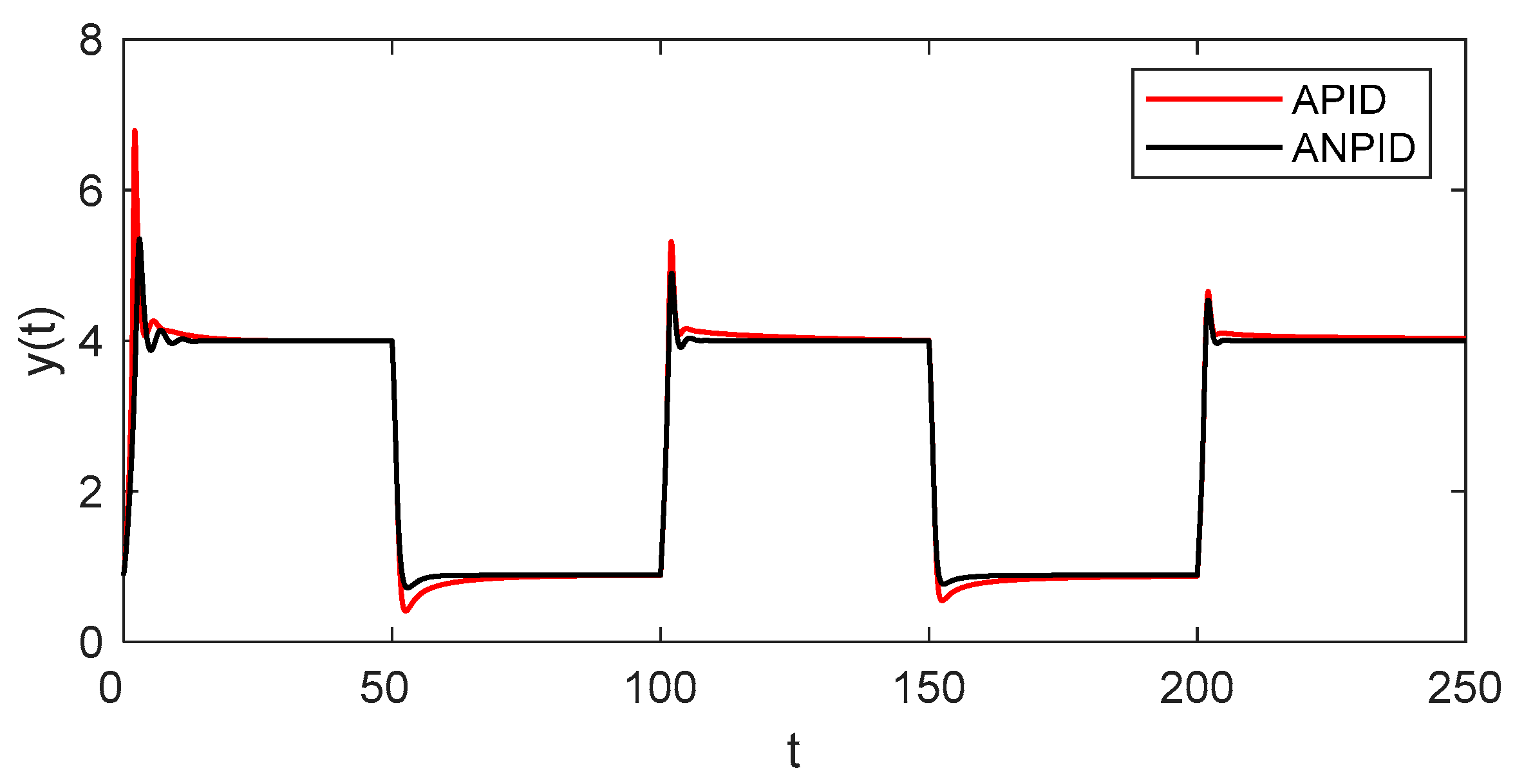
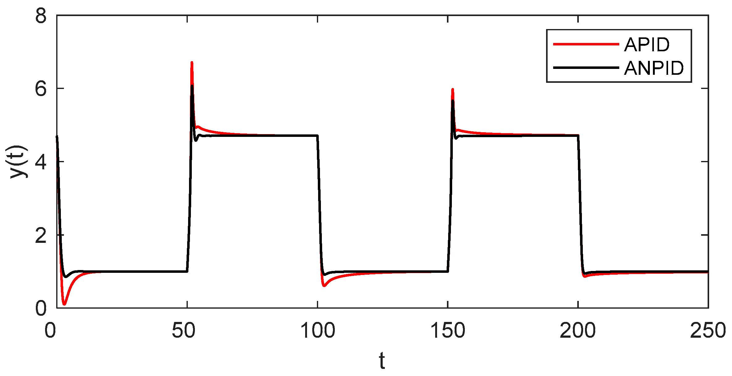
An experiment was conducted to evaluate the ANPID controller’s setpoint tracking performance. Starting from a stable equilibrium point [0.144, 0.886]T, a square wave signal, alternating between 0.886 and 4, was used as the setpoint until t reached 250. The resulting responses, along with those obtained by the APID controller, are presented in Figure 9. Figure 10 shows the system’s output responses to a series of downward and upward setpoint changes starting from another stable equilibrium point [0.765, 4.705]T, alternating between 1 and 4.705. The results demonstrate that both adaptive controllers, even starting with the challenging initial response, effectively stabilize the system response around the setpoint, achieving good control performance. The ANPID controller exhibits better setpoint tracking performance with less overshoot compared to the APID controller.
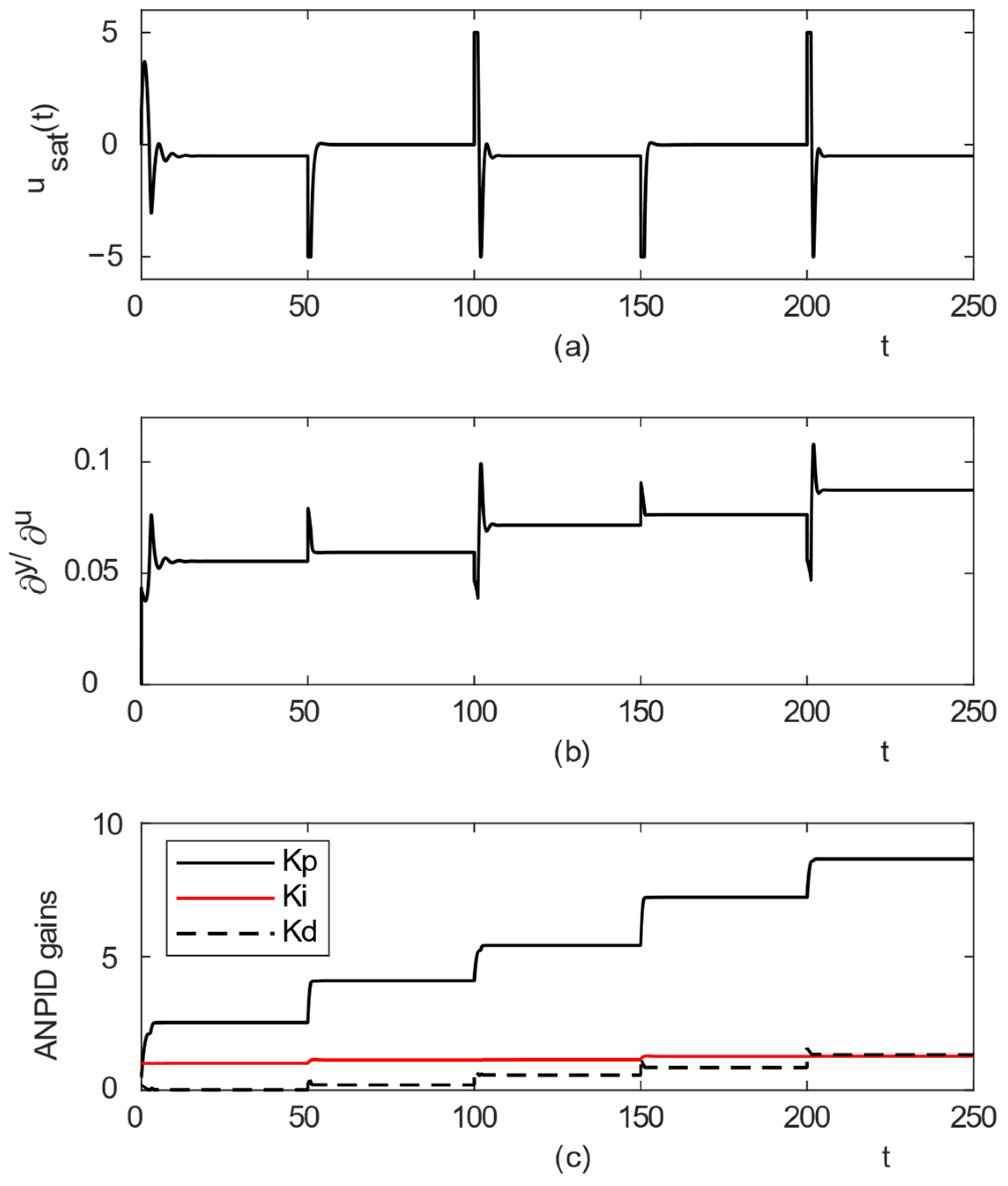
Both methods demonstrate progressively improved responses over time, confirming the effectiveness of their respective adaptation mechanisms. However, comparative analysis reveals that the proposed method achieves superior performance with reduced overshoot and faster transient decay. The adaptation process of the ANPID controller is shown in Figure 11. Figure 11a illustrates the saturated control input, Figure 11b depicts the sensitivity of the output to changes in the control input, and Figure 11c shows the adaptation of the NPID controller gains.
To quantify the performance of the two methods, Table 2 and Table 3 summarize the aforementioned performance indices for the responses to the last two setpoint changes. Additionally, the total performance of both methods was assessed using the IAE calculated over the entire simulation period for two scenarios. For a series of upward and downward setpoint changes, the IAEs of the ANPID and APID controllers are 19.213 and 30.725, respectively. For the other scenario, their IAEs are 19.883 and 32.117, respectively. The superiority of the proposed method can be confirmed again through quantitative comparison.
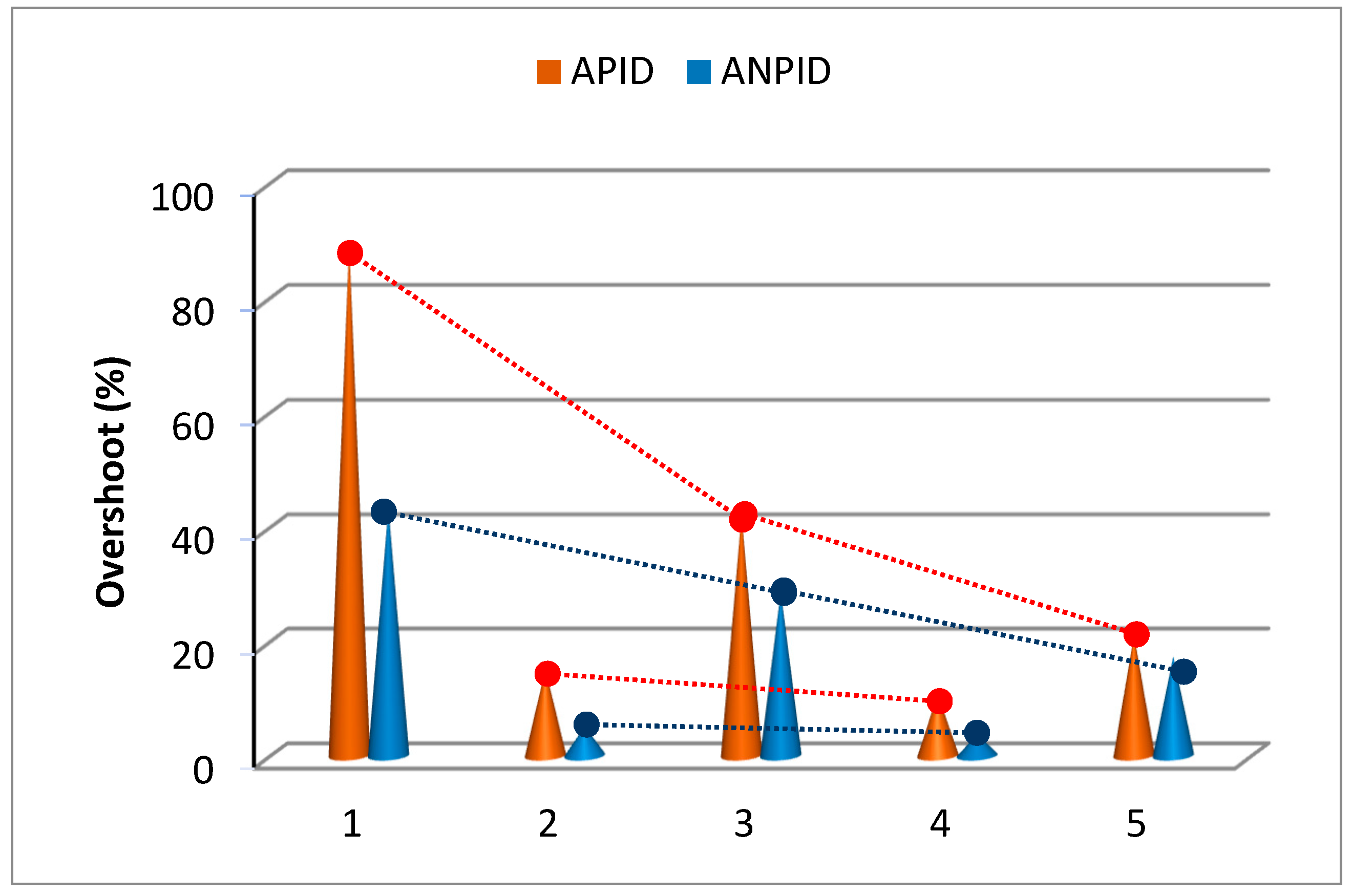
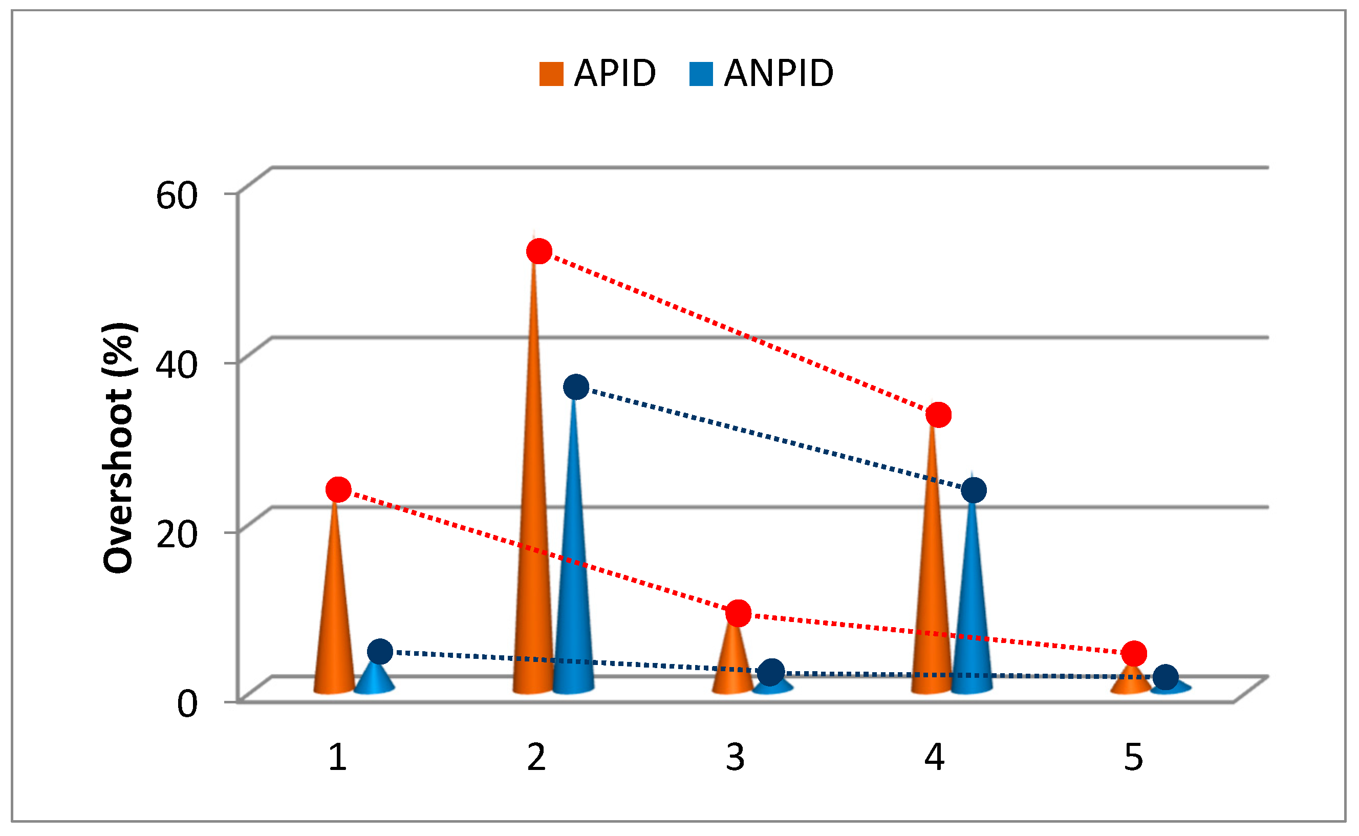
Figure 12 and Figure 13 depict overshoot tendencies for both methods. These figures demonstrate that the adaptation mechanism effectively reduces overshoot in both cases.

4.3. Disturbance Rejection Performance

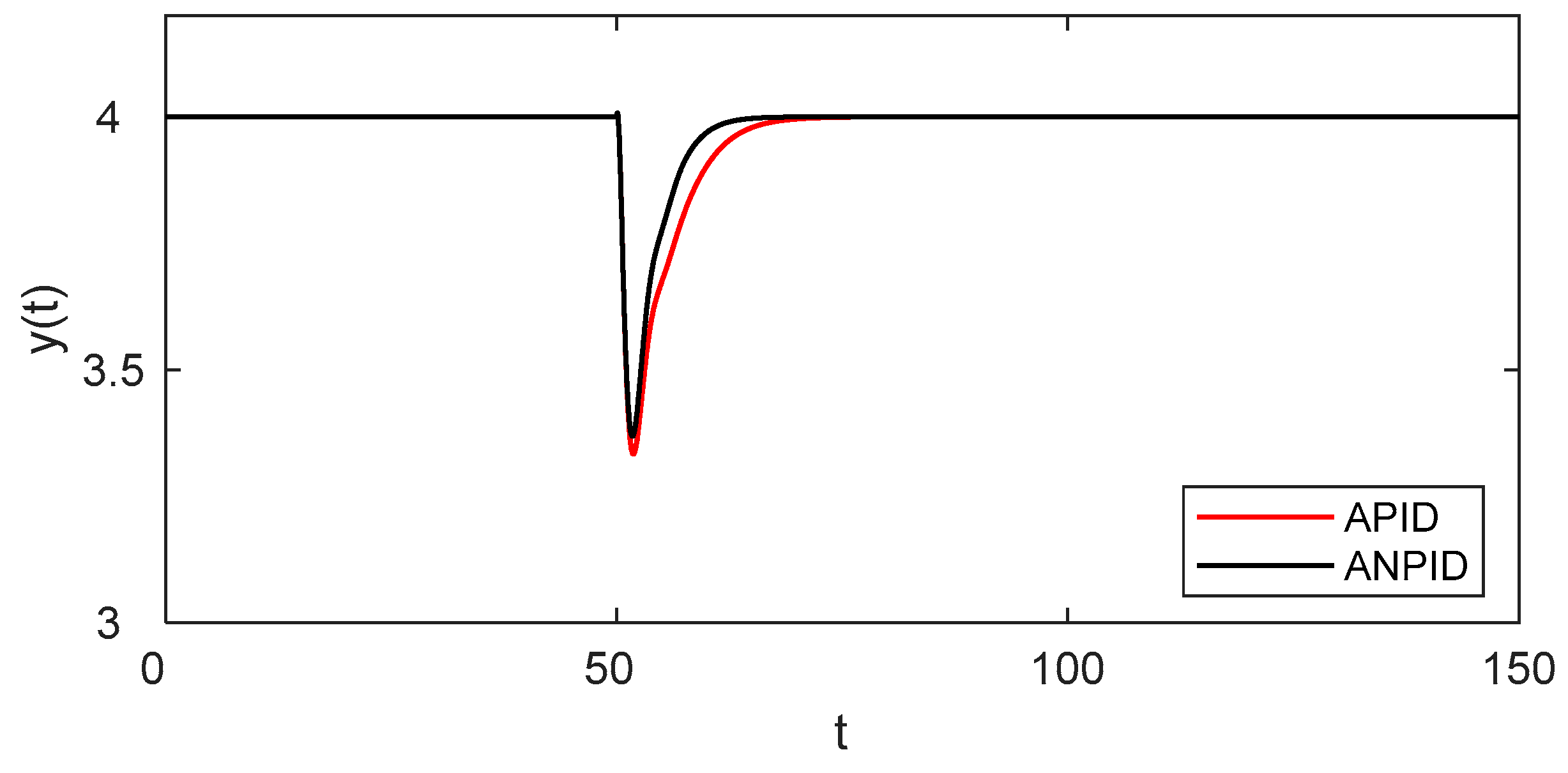
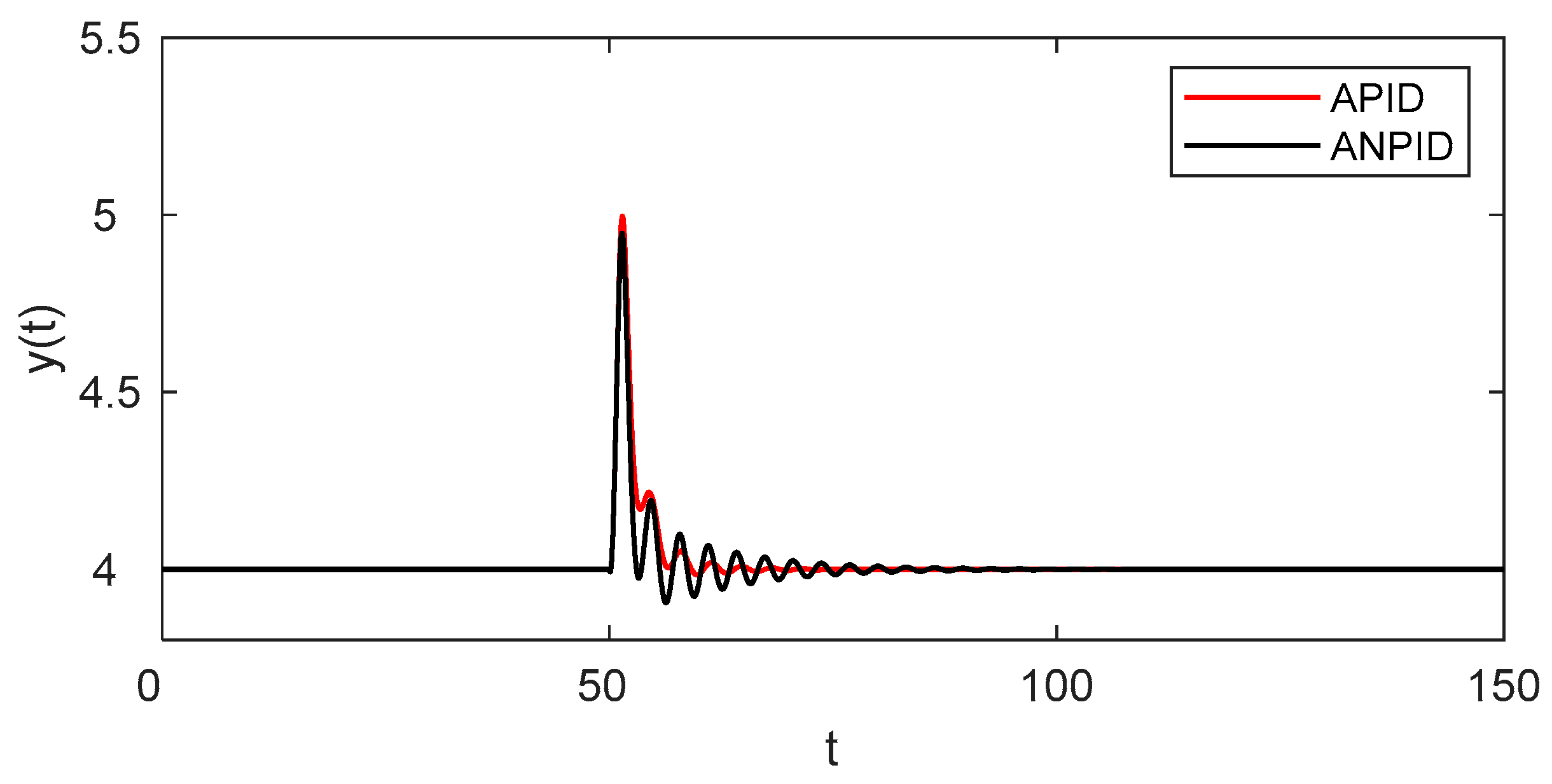
Subsequently, two simulations were then conducted on the nonlinear CSTR model in (4) to evaluate the proposed method’s effectiveness in mitigating disturbances. In the first simulation, stepwise disturbances (d1 = 0.2 and d2 = 0.2) were introduced at t = 50, while the output was maintained at the desired setpoint (yr = 4). Figure 14 compares the response of the proposed method with that of the APID controller.
When the output of the process stayed at yr = 4, stepwise disturbances of d1 = −0.2 and d2 = −0.2 were injected to the control input at t = 50. The responses are plotted in Figure 15. As can be seen from the two figures, the outputs of both methods exhibit rapid recovery from disturbances and remains at the setpoint.
Table 4 summarizes the calculated values of Mpeak, trcy, and IAE. A quantitative analysis of these results reveals the effectiveness of both methods in rejecting disturbances.

4.4. Robustness to Parameter Variations

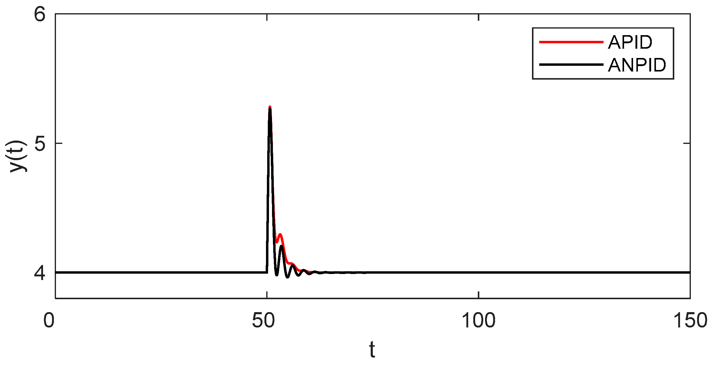
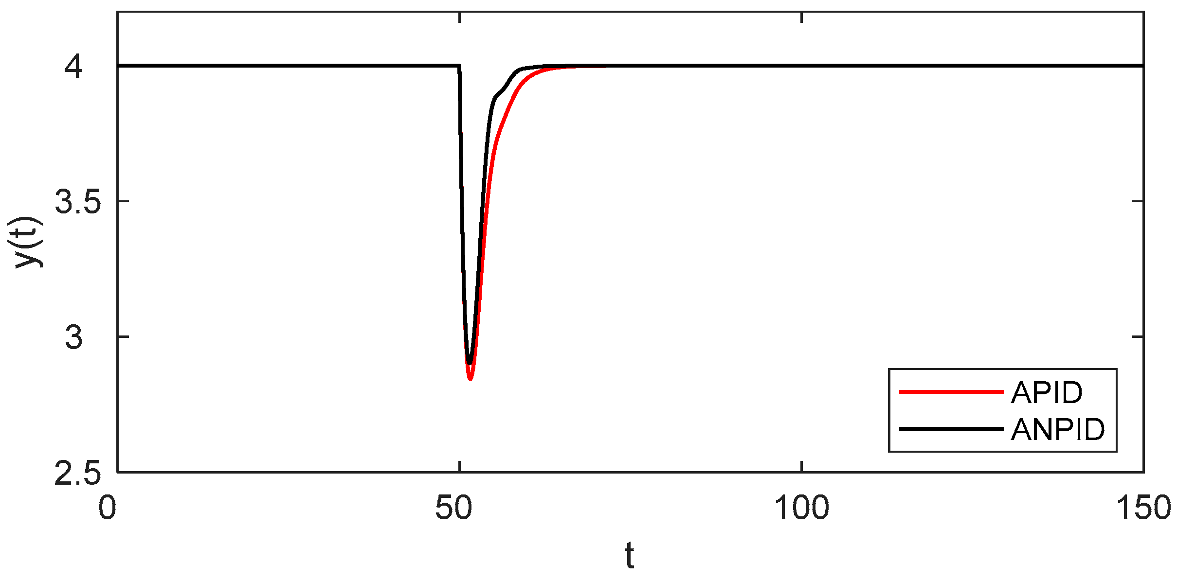
Robust controllers are crucial for maintaining consistent performance in the face of varying system parameters. The robustness of the proposed controller was assessed by perturbing the key parameters Da, H, and β, which significantly influence CSTR dynamics, by ±20% around their nominal values (Da = 0.072, H = 8, and β = 0.3).
Figure 16 shows the system’s behavior with increased parameters (Da = 0.0864, H = 9.6, β = 0.36), while Figure 17 depicts the system’s response to decreased parameters (Da = 0.0576, H = 6.4, β = 0.24). Table 5 quantifies the performance metrics associated with these variations.
An analysis of the figures and table reveals that the outputs of both methods demonstrate a swift return to the setpoint following parameter variations. These findings support the efficacy of the adaptation mechanism in the two methods.

5. Conclusions

This study addressed temperature control in a CSTR process by employing nonlinear PID control in conjunction with a neural network. The process dynamics were identified using an RBFNN, whose weights, centers, and widths were continuously updated with an online learning rule. Simultaneously, the gains of the nonlinear PID controller, incorporating saturation commonly observed in real-world systems, were updated online to achieve superior performance. To evaluate the feasibility of the proposed method, a series of simulations were conducted to assess its performance in tracking, disturbance rejection, and parameter variation scenarios. The results of these simulations were then compared with those obtained from an adaptive RBFNN-based PID controller under identical conditions. The simulation results showed significant improvements with the proposed method compared to the APID controller. For setpoint changes, maximum overshoot decreased by 33.7% and settling time decreased by 54.2% for upward/downward transitions, and these parameters decreased by 27.2% and 5.3% for downward/upward transitions, respectively. Under disturbance changes, reductions were observed in peak magnitude (Mpeak) of 4.9%, in recovery time (trcy) of 23.6%, and in the integral absolute error (IAE) of 16.2%. Similarly, for parameter variations, the reductions were 3.0% (Mpeak), 26.4% (trcy), and 24.4% (IAE). Further research could investigate the practical implementation of this algorithm in a physical system, as well as the design of an adaptive nonlinear TDOF PID controller with a first-order filter in the derivative term.

Author Contributions

J.-Y.L., conceptualization, writing—original draft preparation, funding acquisition; G.-G.J., writing—review and editing, software, visualization; G.-B.S., supervision, writing—review and editing, validation. All authors have read and agreed to the published version of the manuscript.

Funding

This research was supported by the project titled “Development of Advanced Technology for Ocean Energy, Harbor and Offshore Structure (PEA 0321)” funded by the Korea Institute of Ocean Science and Technology (KIOST), South Korea.

Data Availability Statement

All data are presented in the article.

Conflicts of Interest

The authors declare no conflicts of interest.

References

  1. Luyben, W.L. Chemical Reactor Design and Control; John Wiley & Sons, Inc.: Hoboken, NJ, USA, 2007. [Google Scholar]
  2. Mann, U. Principles of Chemical Reactor Analysis and Design, 2nd ed.; John Wiley & Sons, Inc.: Hoboken, NJ, USA, 2009. [Google Scholar]
  3. Dutta, B.; Kumar Tayal, V. PID Controller Design for Continuous Stirred Tank Reactor (CSTR) Temperature Control. In Innovations in Cyber Physical Systems; Singh, J., Kumar, S., Choudhury, U., Eds.; Lecture Notes in Electrical Engineering, Volume 788; Springer: Singapore, 2021. [Google Scholar] [CrossRef]
  4. Jayachitra, A.; Vinodha, R. Genetic Algorithm Based PID Controller Tuning Approach for Continuous Stirred Tank Reactor. Adv. Artif. Intell. 2014, 2014, 791230. [Google Scholar] [CrossRef]
  5. O’Dwyer, A. Handbook of PI and PID Controller Tuning Rules; Imperial College Press: London, UK, 2009. [Google Scholar]
  6. Ranjan, A.; Chakraborty, S. Gain-Scheduled Feedback Controller Design for a Nonlinear Continuous Stirred Tank Reactor. In Proceedings of the 2020 International Conference on Emerging Frontiers in Electrical and Electronic Technologies (ICEFEET), Patna, India, 9–11 July 2020. [Google Scholar] [CrossRef]
  7. Bingi, K.; Ibrahim, R.; Karsiti, M.N.; Hassan, S.M.; Harindran, V.R. A Comparative Study of 2DOF PID and 2DOF Fractional Order PID Controllers on a Class of Unstable Systems. Arch. Control. Sci. 2018, 28, 635–682. [Google Scholar] [CrossRef]
  8. Poovarasan, J.; Kayalvizhi, R.; Pongiannan, R.K. Design of Fractional Order PID Controller for a CSTR Process. Int. Ref. J. Eng. Sci. 2014, 3, 8–14. [Google Scholar]
  9. Wase, M.G.; Gebrekirstos, R.F.; Jin, G.G.; So, G.B. Fuzzy Gain Scheduling of the Fractional-Order PID Controller for a Continuous Stirred-Tank Reactor Process. Processes 2023, 11, 3275. [Google Scholar] [CrossRef]
  10. Seraji, H. A New Class of Nonlinear PID Controllers. In Proceedings of the 5th IFAC Symposium on Robot Control 1997 (SYROCO ‘97), Nantes, France, 3–5 September 1997; pp. 65–71. [Google Scholar]
  11. Seraji, H. A New Class of Nonlinear PID Controllers with Robotic Applications. J. Robot. Syst. 1998, 15, 161–181. [Google Scholar] [CrossRef]
  12. Korkmaz, M.; Aydogdu, O.; Dogan, H. Design and Performance Comparison of Variable Parameter Nonlinear PID Controller and Genetic Algorithm-Based PID Controller. In Proceedings of the 2012 IEEE International Symposium on Innovations in Intelligent Systems and Applications (INISTA), Trabzon, Turkey, 2–4 July 2012; pp. 1–5. [Google Scholar]
  13. Li, Y.; Guo, G.; Wang, Y. A Nonlinear Control Scheme for Fast Settling in Hard Disk Drives. IEEE Trans. Magn. 2004, 40, 2086–2088. [Google Scholar] [CrossRef]
  14. So, G.B.; Jin, G.G. Fuzzy-Based Nonlinear PID Controller and Its Application to CSTR. Korean J. Chem. Eng. 2018, 35, 819–825. [Google Scholar] [CrossRef]
  15. Jin, G.G.; Son, Y.D. Design of a Nonlinear PID Controller and Tuning Rules for First-Order Plus Time Delay Models. Stud. Inform. Control. 2019, 28, 157–166. [Google Scholar] [CrossRef]
  16. Son, Y.D.; Jin, G.G.; Yetayew, T.T.; Pal, P. New Tuning Formulas for a Nonlinear PID Control Scheme. Int. J. Syst. Assur. Eng. Manag. 2023, 14, 2470–2484. [Google Scholar] [CrossRef]
  17. Kalita, P.; Barman, J.K. Performance Analysis of Nonlinear Jacketed CSTR Based on Different Control Strategies. J. Electr. Electron. Eng. 2017, 1, 1–7. [Google Scholar]
  18. Ouyang, M.; Wang, Y.; Wu, F.; Lin, Y. Continuous Reactor Temperature Control with Optimized PID Parameters Based on Improved Sparrow Algorithm. Processes 2023, 11, 1302. [Google Scholar] [CrossRef]
  19. Maya-Rodriguez, M.C.; Carvajal-Mariscal, I.; López-Muñoz, R.; Lopez-Pacheco, M.A.; Tolentino-Eslava, R. Temperature Control of a Chemical Reactor Based on Neuro-Fuzzy Tuned with a Metaheuristic Technique to Improve Biodiesel Production. Energies 2023, 16, 6187. [Google Scholar] [CrossRef]
  20. Vojtesek, J.; Dostal, P. Nonlinear versus Ordinary Adaptive Control of Continuous Stirred-Tank Reactor. Sci. World J. 2015, 2015, 389273. [Google Scholar] [CrossRef] [PubMed]
  21. Anbu, S.; Jaya, N. Design of Model Reference Adaptive Control and Nonlinear PI Controller for Continuous Stirred Tank Reactor. Int. J. Comput. Appl. 2016, 153, 13–16. [Google Scholar] [CrossRef]
  22. Li, D.; Wang, D.; Gao, Y. Adaptive Neural Control and Modeling for Continuous Stirred Tank Reactor with Delays and Full State Constraints. Complexity 2021, 2021, 9948044. [Google Scholar] [CrossRef]
  23. Zerari, N.; Chemachema, M. Robust Adaptive Neural Network Prescribed Performance Control for Uncertain CSTR System with Input Nonlinearities and External Disturbance. Neural Comput. Appl. 2020, 32, 10541–10554. [Google Scholar] [CrossRef]
  24. Shi, X.; Zhao, H.; Fan, Z. Parameter Optimization of Nonlinear PID Controller Using RBF Neural Network for Continuous Stirred Tank Reactor. Meas. Control 2023, 56, 1835–1843. [Google Scholar] [CrossRef]
  25. Li, D.; Wang, Y.; Liu, Y.-J.; Liu, L. IBLFs-Based Adaptive Fuzzy Control for Continuous Stirred Tank Reactors with Full State Constraints and Actuator Faults. J. Process Control 2023, 124, 14–24. [Google Scholar] [CrossRef]
  26. Sarjaš, A.; Gleich, D. Event-Triggered Sliding Mode Control For Constrained Networked Control Ssystems. Electron. Energetics 2022, 35, 557–570. [Google Scholar] [CrossRef]
  27. Chaturvedi, S.; Kumar, N.; Kumar, R. A PSO-optimized novel PID neural network model for temperature control of jacketed CSTR: Design, simulation, and a comparative study. Soft Comput. 2024, 28, 4759–4773. [Google Scholar] [CrossRef]
  28. Baranilingesan, I.; Deepa, S.N.; Yagambal Jayalaskshmi, N. An Intelligent Neural Network Controller for Non-Linear CSTR Process Control. Iran. J. Chem. Chem. Eng. 2023, 42, 977–988. [Google Scholar] [CrossRef]
  29. Zhang, G.; Li, Z.; Li, J.; Zhang, W.; Qiu, B. Prescribed Performance Path-Following Control for Rotor-Assisted Vehicles via an Improved Reinforcement Learning Mechanism. IEEE Trans. Neural Netw. Learn. Syst. 2025, 1–12. [Google Scholar] [CrossRef] [PubMed]
  30. Liu, R.; He, Y.; Zhao, Y.; Jiang, X.; Ren, S. Tunnel construction ventilation frequency-control based on radial basis function neural network. Autom. Constr. 2020, 118, 103293. [Google Scholar] [CrossRef]
  31. Ray, W.H. Advanced Process Control; McGraw-Hill: New York, NY, USA, 1981. [Google Scholar]
  32. Soukkou, A.; Khellaf, S.; Leulmi, S.; Boudeghdegh, K. Optimal Control of a CSTR Process. Braz. J. Chem. Eng. 2008, 25, 799–812. [Google Scholar] [CrossRef]
  33. Suo, L.; Ren, J.; Zhao, Z.; Zhai, C. Study on the Nonlinear Dynamics of the Continuous Stirred Tank Reactors. Processes 2020, 8, 1436. [Google Scholar] [CrossRef]
  34. Hagan, M.T.; Demuth, H.B.; Beale, M.H.; De Jesús, O. Neural Network Design, 2nd ed.; Martin Hagan; PWS Publishing Co.: Boston, MA, USA, 2014. [Google Scholar]
  35. Raff, L.; Komanduri, R.; Hagan, M.T.; Bukkapatnam, S. Neural Networks in Chemical Reaction Dynamics; Oxford University Press: Oxford, UK, 2012. [Google Scholar]
  36. Srinivas, N.; Deb, K. Multiobjective Optimization Using Nondominated Sorting in Genetic Algorithms. Evol. Comput. 1994, 2, 221–248. [Google Scholar] [CrossRef]
  37. Deb, K.; Pratap, A.; Agarwal, S.; Meyarivan, T. A Fast and Elitist Multiobjective Genetic Algorithm: NSGA-II. IEEE Trans. Evol. Comput. 2002, 6, 182–197. [Google Scholar] [CrossRef]
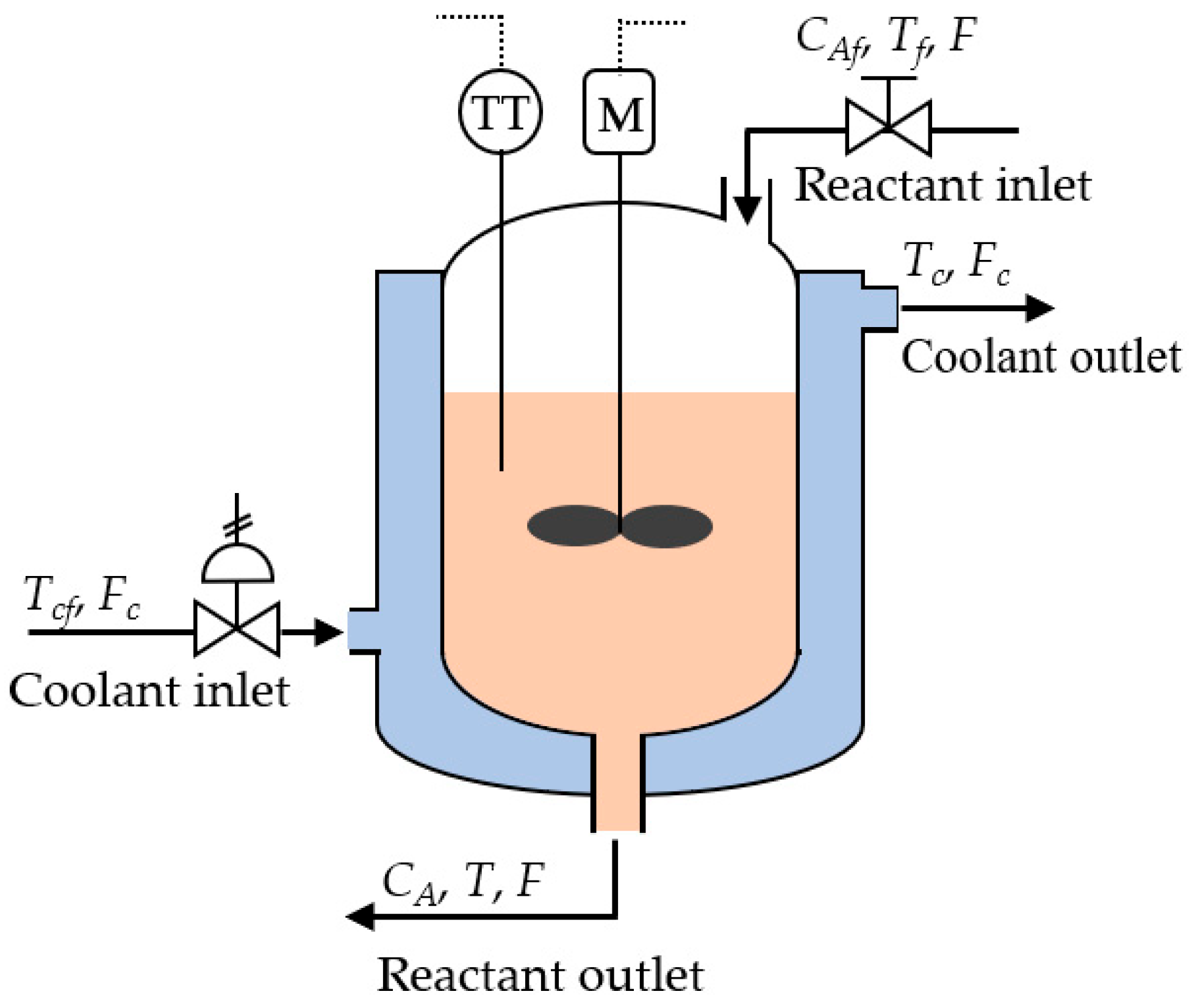
Figure 1. A schematic diagram of the CSTR process with a cooling jacket.
Algorithms 18 00442 g001
Figure 2. Phase portrait and three equilibria.
Algorithms 18 00442 g002
Figure 3. Output responses of CSTR.
Algorithms 18 00442 g003
Figure 4. Structure of RBFNN with three layers.
Algorithms 18 00442 g004
Figure 5. Structure of NPID controller.
Algorithms 18 00442 g005
Figure 6. Scaled error plots for different Δr values.
Algorithms 18 00442 g006
Figure 7. Optimal Pareto fronts of NPID and PID controllers: (a) L/T = 0.01; (b) L/T = 0.1; (c) L/T = 0.5; (d) L/T = 1.
Algorithms 18 00442 g007
Figure 8. Proposed adaptive NPID control scheme based on RBFNN.
Algorithms 18 00442 g008
Figure 9. Output responses to a series of upward and downward setpoint changes.
Algorithms 18 00442 g009
Figure 10. Output responses to a series of downward and upward setpoint changes.
Algorithms 18 00442 g010
Figure 11. Adaptation process of ANPID controller: (a) The saturated control input; (b) The sensitivity of the output to change in the control input; (c) The adaptation of ANPID controller gains.
Algorithms 18 00442 g011
Figure 12. Overshoot tendencies when the setpoint is repeatedly adjusted upwards and downwards.
Algorithms 18 00442 g012
Figure 13. Overshoot tendencies when the setpoint is repeatedly adjusted downwards and upwards.
Algorithms 18 00442 g013
Figure 14. Disturbance performance when d1 = 0→0.2 and d2 = 0→0.2.
Algorithms 18 00442 g014
Figure 15. Disturbance performance when d1 = 0→−0.2 and d2 = 0→−0.2.
Algorithms 18 00442 g015
Figure 16. Responses of two methods to increased parameters.
Algorithms 18 00442 g016
Figure 17. Responses of two methods to decreased parameters.
Algorithms 18 00442 g017
Table 1. Parameters of CSTR.
ParameterDescription
CAReactant concentration
CAfReactant inlet concentration
TReactant temperature
TfReactant inlet temperature
FReactant flow rate
TcCoolant temperature
TcfCoolant inlet temperature
FcCoolant flow rate
ρReactant density
CpReactant volumetric heat capacity
ρjCoolant density
CpjCoolant volumetric heat capacity
UAHeat transfer item
ΔHReaction heat
k0Reaction rate constant
EActivation energy
RGas constant
VReactor volume
VjJacket volume
τTime
Table 2. Performance indices for the last two downward and upward setpoint changes.
Controlleryr = 4 → 0.886yr = 0.886 → 4
MptrtsIAEMptrtsIAE
APID10.7921.1236.4915.40621.1521.1892.8855.842
ANPID3.7551.2031.5652.86717.4161.2132.7303.265
Table 3. Performance indices for the last two upward and downward setpoint changes.
Controlleryr = 1 → 4.705yr = 4.705 → 1
MptrtsIAEMptrtsIAE
APID34.2691.1722.7596.5743.7061.2491.5795.109
ANPID26.0041.1882.4754.2521.6601.2701.6333.383
Table 4. Disturbance rejection performance comparison of the two methods.
Controllerd1 = 0 → 0.2, d2 = 0 → 0.2d1 = 0 → −0.2, d2 = 0 → −0.2
MpeaktrcyIAEMpeaktrcyIAE
APID0.66613.5293.5060.99618.1502.232
ANPID0.6319.9162.5100.94914.2792.296
Table 5. Performance comparison of parameter variations of two methods.
ControllerDa = 0.0864, H = 9.6, β = 0.36Da = 0.0576, H = 6.4, β = 0.24
MpeaktrcyIAEMpeaktrcyIAE
APID1.2836.1472.3061.1559.4014.686
ANPID1.2664.1511.7741.0987.2873.511
Disclaimer/Publisher’s Note: The statements, opinions and data contained in all publications are solely those of the individual author(s) and contributor(s) and not of MDPI and/or the editor(s). MDPI and/or the editor(s) disclaim responsibility for any injury to people or property resulting from any ideas, methods, instructions or products referred to in the content.