Iterative Matrix Techniques Based on Averages

Abstract

Matrices have an important role in modern engineering problems like artificial intelligence, biomedicine, machine learning, etc. The present paper proposes new algorithms to solve linear problems involving finite matrices as well as operators in infinite dimensions. It is well known that the power method to find an eigenvalue and an eigenvector of a matrix requires the existence of a dominant eigenvalue. This article proposes an iterative method to find eigenvalues of matrices without a dominant eigenvalue. This algorithm is based on a procedure involving averages of the mapping and the independent variable. The second contribution is the computation of an eigenvector associated with a known eigenvalue of linear operators or matrices. Then, a novel numerical method for solving a linear system of equations is studied. The algorithm is especially suitable for cases where the iteration matrix has a norm equal to one or the standard iterative method based on fixed point approximation converges very slowly. These procedures are applied to the resolution of Fredholm integral equations of the first kind with an arbitrary kernel by means of orthogonal polynomials, and in a particular case where the kernel is separable. Regarding the latter case, this paper studies the properties of the associated Fredholm operator.

1. Introduction

Matrices have an important role in current engineering problems like artificial intelligence [1], biomedicine [2], machine learning [3], neural networks [4], etc. It could be said that they are, in fact, an interface between mathematics and the real world. Spectral matrix theory is closely related to big data and statistics, graph theory, networking, cryptography, search engines, optimization, convexity and, of course, the resolution of all kinds of linear equations.

An open problem of spectral theory is the sought-for eigenvalues and eigenvectors of a matrix. For this purpose, iterative methods are especially appropriate when the matrices have a large size and they are sparse, because the iteration matrix does not change during the process.

The classical power method of R. von Mises and H. Pollaczek-Geiringer [5] assumes the existence of a dominant eigenvalue. One of the main contributions of this paper is the proposal of an algorithm to compute the eigenvalues of matrices and operators that do not have a dominant eigenvalue. The algorithm is based on the iterative averaged methods for fixed-point approximation proposed initially by Mann [6] and Krasnoselskii [7] and, subsequently, by Ishikawa [8], Noor [9], Sahu [10] and others. There are recent articles on this topic (references [11,12,13,14,15,16,17,18,19], for instance). In general, these papers deal with the problem of approximation of fixed points of non-expansive, asymptotically non-expansive and nearly asymptotically non-expansive mappings that are particular cases of Lipschitz and near-Lipschitz maps [20,21]. However, this article aims to prove that the usefulness of iterative averaged methods goes beyond fixed-point approximation.

In reference [22], the author proposed a new algorithm of this type called N-iteration. The method has proved useful for the iterative resolution of Fredholm integral equations of the second kind and of the Hammerstein type [23] (see, for instance, references [24,25]).

The above procedure is used in this article to compute eigenvalues and eigenvectors of matrices and linear operators (Section 2 and Section 3) and for the resolution of systems of linear equations (Section 4). All these techniques are applied to solving Fredholm integral equations [26,27,28,29,30] of the first kind by means of orthogonal polynomials (Section 5). In Section 6, we review some properties of compact and Fredholm integral operators, while Section 7 presents the solution of a Fredholm integral equation of the first kind in a particular case where the kernel of the operator is separable. Section 8 deals with a particular case of a Fredholm integral equation of the second kind. Several examples with tables and figures illustrate the performance and convergence of the algorithms proposed.

2. Averaged Power Method for Finding Eigenvalues and Eigenvectors of a Matrix

Given a matrix $A\in \mathcal{M}(m\times m)$, where $\mathcal{M}(m\times m)$ denotes the set of real or complex matrices of size $m\times m$, the power method is a well-known procedure for finding the dominant eigenvalue of matrix A. Let $\sigma \left(A\right)$ represent the spectrum of A, that is to say, the set of eigenvalues of A.

Definition 1. 

A matrix A has a dominant eigenvalue ${\lambda }_1\in \sigma \left(A\right)$ if $|{\lambda }_1|>|{\lambda }_j|$ for any ${\lambda }_j\in \sigma \left(A\right)$, $j\ne 1.$ If $v\in {\mathbb{R}}^m$ (or $v\in {\mathbb{C}}^m$) is non-null and $Av={\lambda }_{1}v$ then v is a dominant eigenvector of $A.$

It is well known that if the matrix A is diagonalizable and it has a dominant eigenvalue, then the sequence defined by $X_0\ne \overline{0}$ and the recurrence $X_{k+1}=A{X}_k$ for $k\ge 0$ converges with high probability to a dominant eigenvector (i.e., if the component of $X_0$ with respect to the dominant eigenvector is non-null). The dominant eigenvalue can be approximated by means of the so-called Rayleigh quotient:

$${\lambda }_1\simeq {\displaystyle \frac{<A{X}_k,X_k>}{<X_k,X_k>}},$$

when k is sufficiently large. The formula comes, obviously, from the definition of an eigenvector associated with the eigenvalue ${\lambda }_1.$ We shall see, with an example, that if the matrix has no dominant eigenvalue then the power method may not converge.

Example 1. 

The matrix $A=diag(1,-1)$ has the eigenvalue ${\lambda }_1=1$ with eigenvectors $(x,0)$ and ${\lambda }_2=-1$ with eigenvectors $(0,y).$ The power method does not work in general since

$$A^k(x,y)=(x,-y),$$

for k being odd and

$$A^k(x,y)=(x,y)$$

for k being even. The sequence ($A^k{X}_0$) does not converge except for the starting point $X_0=(x,0).$

The present section is devoted to proposing an algorithm to find eigenvalues and eigenvectors of matrices that do not have a dominant eigenvalue.

In reference [22], an algorithm for the approximation of a fixed point of $T:C\to C,$ where C, is a nonempty, closed and convex subset of a proposed normed space E. This is given by the following recurrence:

$$\begin{array}{cc}\hfill g_n& =(1-{\alpha }_n)f_n+{\alpha }_{n}T{f}_n,\hfill \\ \hfill h_n& =(1-{\beta }_n)f_n+{\beta }_n{g}_n,\hfill \\ \hfill f_{n+1}& =(1-{\gamma }_n)h_n+{\gamma }_{n}T{h}_n,\hfill \end{array}$$

for ${\alpha }_n,{\beta }_n,{\gamma }_n\in [0,1],$$n\ge 0$ and $f_0\in C.$ This iterative scheme was called N-algorithm. The procedure generalizes the Krasnoselskii–Mann method, defined in references [6,7], obtained in the case where ${\alpha }_n=0,{\beta }_n=1$. If, additionally, ${\gamma }_n=1$ one has the usual Picard–Banach iteration.

Averaged power method

If the matrix $A\in \mathcal{M}(m\times m)$ has no dominant eigenvalue, that is to say, $|{\lambda }_j|=k\ne 0$ for any ${\lambda }_j\in \sigma \left(A\right)$, the power method may not converge. The algorithm proposed here is the use of the N-iteration of the matrix A instead of computing the powers of A. The sequence of vectors obtained by the power or the averaged power method may produce a divergent sequence (even though the iterates may be good approximations of an eigenvector). To avoid this fact, a scaling of the output vector is sometimes performed at every step of the algorithm. Thus, the procedure is described by the following recurrence:

$$\begin{array}{cc}\hfill & V_n=(1-{\alpha }_n)X_n+{\alpha }_{n}A{X}_n,\hfill \\ \hfill & W_n=(1-{\beta }_n)X_n+{\beta }_n{V}_n,\hfill \\ \hfill & X_{n+1}=(1-{\gamma }_n)W_n+{\gamma }_{n}A{W}_n,\hfill \\ \hfill & X_{n+1}:=X_{n+1}/\left|\right|X_{n+1}\left|\right|,\hfill \\ \hfill & {\lambda }_{n+1}=<A{X}_{n+1},X_{n+1}>\hfill \end{array}$$

for ${\alpha }_n,{\beta }_n,{\gamma }_n\in [0,1],$ such that $0<inf{\alpha }_n\le sup{\alpha }_n<1,$$0<inf{\gamma }_n\le sup{\gamma }_n<1,$ and $X_0\ne \overline{0},$ $X_0\in {\mathbb{R}}^m.$ The notation $\left|\right|·\left|\right|$ represents any norm in ${\mathbb{R}}^m$ and $<·,·>$ is the inner product in the m-dimensional Euclidean space.

A useful criterion to stop the algorithm is to check that $\left|\right|A{X}_{n+1}-{\lambda }_{n+1}{X}_{n+1}\left|\right|<\epsilon$ for some tolerance $\epsilon ,$ or $|{\lambda }_{n+1}-{\lambda }_n|<\epsilon$.

The last value ${\lambda }_k$ is an approximation of an eigenvalue of A and $X_k$ is the corresponding eigenvector.

In order to justify the suitability of the algorithm, we will consider the simplest case of the Krasnoselskii iteration:

$$X_{n+1}=(1-\alpha )X_n+\alpha A{X}_n=((1-\alpha )I+\alpha A)X_n,$$

for $0<\alpha <1.$ Let us denote $B:=(1-\alpha )I+\alpha A.$ It is easy to check that

$$\sigma \left(B\right)=\left\{\right(1-\alpha )+\lambda \alpha :\lambda \in \sigma (A\left)\right\},$$

and the eigenvectors of B and A agree, that is to say, X is an eigenvector of A with respect to an eigenvalue $\lambda$, if and only if X is an eigenvector of B with eigenvalue $(1-\alpha )+\lambda \alpha .$

Let us assume that A has positive and negative eigenvalues with the same absolute value. Then, $|(1-\alpha )+\alpha \lambda |\le (1-\alpha )+\alpha {\lambda }^{*}$ for the positive eigenvalue ${\lambda }^{*}.$

For a negative eigenvalue $\lambda :$$|(1-\alpha )+\alpha \lambda |<(1-\alpha )+\alpha {\lambda }^{*}$ and, consequently, $(1-\alpha )+\alpha {\lambda }^{*}$ is a dominant eigenvalue of B. Hence, the power method applied to the matrix B will converge to an eigenvector of B (and thus of A), if the component of $X_0$ with respect to this eigenvector is non-null.

The power method is based on the product of a matrix $A\in \mathcal{M}(m\times m)$ and a vector. This operation has a complexity $\mathcal{O}\left(m^2\right).$ If the number of iterations is $n_{max}$, the complexity is $\mathcal{O}\left(n_{max}{m}^2\right).$ For a large matrix, the averaging operations of the N-algorithm proposed are negligible, and the complexity is $\mathcal{O}\left(2n_{max}{m}^2\right).$ Though the operations involved are about twice as many as in the original power method, the type of convergence (polynomial of degree 2) is not modified. If one wishes to reduce the total number of operations, the use of constant weight coefficients is advisable, and the algorithm is able to be conveniently optimized.

The speed of convergence of the power method (and consequently the number of iterations required to give a good approximation) depends on the ratio $|{\lambda }_2|/|{\lambda }_1|,$ where ${\lambda }_1,{\lambda }_2$ are the greatest eigenvalues in magnitude. The smaller is this quotient, while the faster is the convergence. In the averaged Mann–Krasnoselskii method, this “spectral gap” is $|1-\alpha -\alpha {\lambda }^{*}|/(1-\alpha +\alpha {\lambda }^{*}),$ where ${\lambda }^{*}$ is the positive eigenvalue. For instance, if $\alpha =1/2$, minimum quotients are reached for values of ${\lambda }^{*}$ close to $1.$

Example 2. 

Considering the matrix of Example 1,

$$A=\left(\begin{array}{cc}1& 0\\ 0& -1\end{array}\right)$$

we obtain that for $X_0=(x,y),$$x\ne 0,$ the Krasnoselskii method with $\alpha =1/2$ gives as first approximation

$$X_1=(X_0+A{X}_0)/2=(x,0),$$

and the rest of iterations agree with the eigenvector $(x,0).$ The positive eigenvalue is computed as ${\lambda }_1=<A{X}_k,X_k>/<X_k,X_k>=x^2/x^2=1.$

Example 3. 

The spectrum of the matrix

$$A=\left(\begin{array}{cc}0& 2\\ 2& 0\end{array}\right)$$

is $\sigma \left(A\right)=\{2,-2\}.$ The N-iteration, with ${\alpha }_n={\beta }_n={\gamma }_n=1/2$ starting at $X_0=(2,-3)$, with Euclidean scaling produces the sequence of approximations collected in

Table 1. Approximations of an eigenvector and successive Euclidean distances.

Iteration (n)	${\mathit{X}}_{\mathit{n}}$	$\left|\right|{\mathit{X}}_{\mathit{n}}-{\mathit{X}}_{\mathit{n}-1}\left|\right|$
1	(−0.894427, −0.447214)	3.85933
2	(−0.691223, −0.722642)	0.342276
3	(−0.708154, −0.706058)	0.023699
4	(−0.707037, −0.707177)	0.001580
5	(−0.707111, −0.707102)	0.000105
6	(−0.707106, −0.707107)	0.000007
7	(−0.707107, −0.707107)	0.000000

.

The eigenvalue computed is $\lambda =<A{X}_7,X_7>/<X_7,X_7>=2.$ The stopping criterion was $\left|\right|X_n-X_{n-1}\left|\right|<{10}^{-6}.$

Example 4. 

Let us consider the following matrix:

$$A=\left(\begin{array}{ccc}-2& 4& 1\\ 0& 3& 0\\ 5& -4& 2\end{array}\right).$$

The set of eigenvalues of A is $\sigma \left(A\right)=\{3,-3\}.$ The algorithm described with ${\alpha }_n={\beta }_n={\gamma }_n=1/2$ starting at $X_0=(2,-3,2)$ with Euclidean scaling produces the sequence of approximations and distances as between those collected in

Table 2. Approximations of an eigenvector with successive distances.

Iteration (n)	${\mathit{X}}_{\mathit{n}}$	$\left|\right|{\mathit{X}}_{\mathit{n}}-{\mathit{X}}_{\mathit{n}-1}\left|\right|$
1	(−0.212899, −0.479022, 0.851594)	3.545573
2	(−0.212899, −0.479022, 0.851594)	0.000001
3	(−0.212899, −0.479022, 0.851594)	0.000000

.

The eigenvalue computed is $\lambda =<A{X}_3,X_3>/<X_3,X_3>=3.$ The stopping criterion was $\left|\right|X_n-X_{n-1}\left|\right|<{10}^{-6}.$

Remark 1. 

Let us notice that the matrices of these examples do not have a dominant eigenvalue but, nevertheless, the N-iterated power algorithm is convergent.

Averaged Power Method for Finding Eigenvalues and Eigenfunctions of a Linear Operator

The algorithm proposed in this section can be applied to find eigenvalues and eigenvectors/eigenfunctions of a linear operator defined in an infinite-dimensional normed linear space $K:E\to E,$ in case of existence (see, for instance, Theorem 2). Starting at $f_0\in E$, we would follow the steps

$$\begin{array}{cc}\hfill & g_n=(1-{\alpha }_n)f_n+{\alpha }_{n}K{f}_n,\hfill \\ \hfill & h_n=(1-{\beta }_n)f_n+{\beta }_n{g}_n,\hfill \\ \hfill & f_{n+1}=(1-{\gamma }_n)f_n+{\gamma }_{n}K{f}_n,\hfill \\ \hfill & f_{n+1}:=f_{n+1}/\left|\right|f_{n+1}\left|\right|,\hfill \\ \hfill & {\lambda }_{n+1}=<K{f}_{n+1},f_{n+1}>\hfill \end{array}$$

for ${\alpha }_n,{\beta }_n,{\gamma }_n\in [0,1],$ such that $0<inf{\alpha }_n\le sup{\alpha }_n<1,$$0<inf{\gamma }_n\le sup{\gamma }_n<1,$ and $f_0\ne \overline{0}.$

Let us note that a structure of inner product space in E for computing the eigenvalue by means of the Rayleigh quotient is required. Otherwise, we should solve the equation $K{f}_n={\lambda }_n{f}_n.$

The stop criteria of the algorithm are similar to the given for matrices, using the norm of the space E or the modulus in the case of employing the approximations of the eigenvalue.

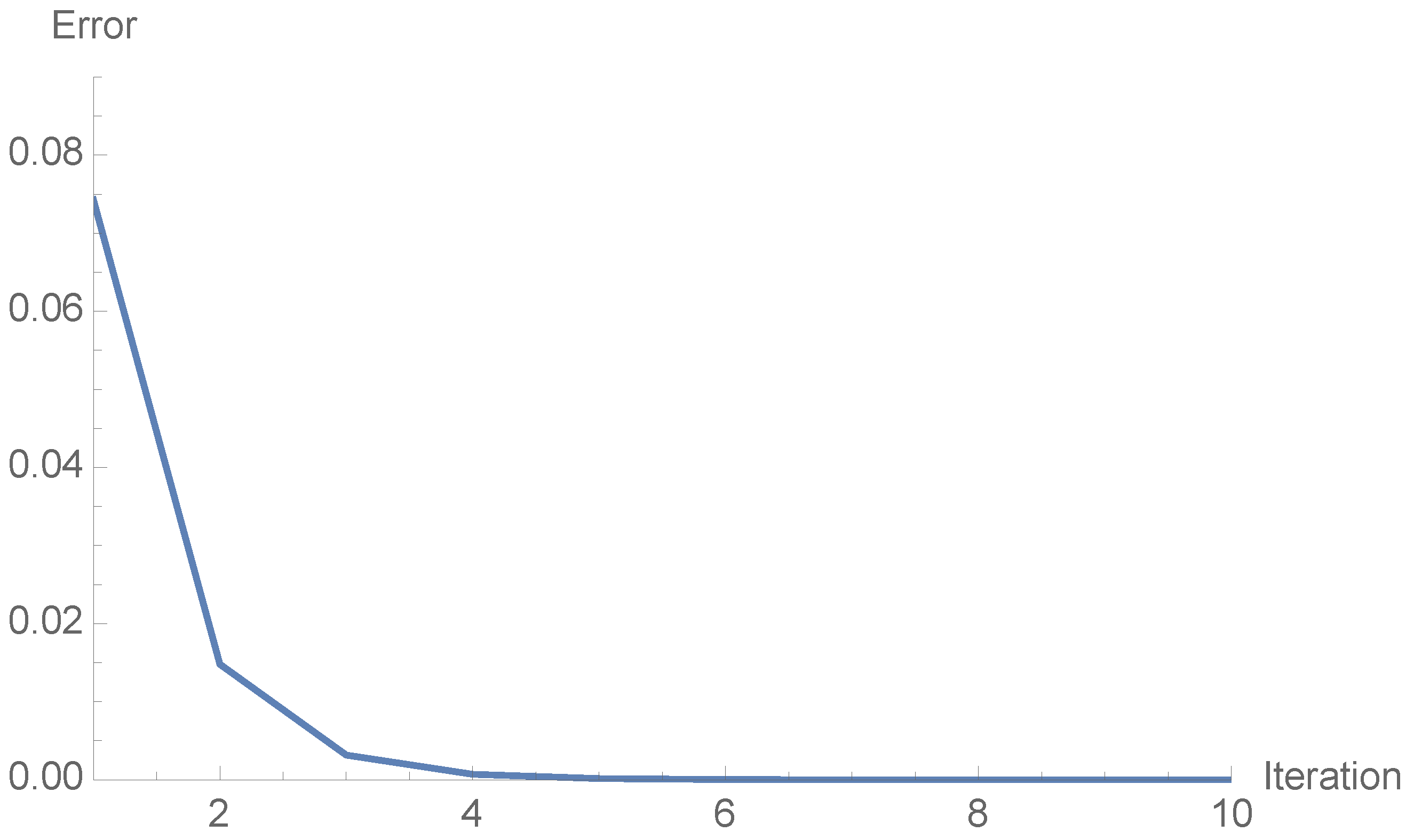
Example 5. 

Let us compute an eigenvalue of a Fredhom integral operator on ${\mathcal{L}}^2\left([0,1]\right)$ defined, for $f\in {\mathcal{L}}^2\left([0,1]\right),$ as

$$Kf\left(x\right):={\int }_0^1(2x^2+3y^3)f\left(y\right)dy,$$

For $f_0\left(x\right)=x$ the sequence of approximate dominant eigenvalues (${\lambda }_n$) generated by the N-algorithm with ${\alpha }_n={\beta }_n={\gamma }_n=1/2$ is collected in

Table 3. Approximations of an eigenvalue of the operator K.

Iteration (n)	${\mathit{\lambda }}_{\mathit{n}}$	$\left|\right|{\mathbf{Kf}}_{\mathit{n}}-{\mathit{\lambda }}_{\mathit{n}}{\mathit{f}}_{\mathit{n}}{\left|\right|}_2$	$|{\mathit{\lambda }}_{\mathit{n}}-{\mathit{\lambda }}_{\mathit{n}-1}|$
1	1.709247	0.074275	-
2	1.709316	0.014805	0.000069
3	1.709179	0.003165	0.000137
4	1.709186	0.000707	0.000007
5	1.709196	0.000162	0.000010
6	1.709201	0.000038	0.000004
7	1.709201	0.000009	0.000001
8	1.709201	0.000002	0.000000
9	1.709201	0.000000	0.000000
10	1.709201	0.000000	0.000000

. The norm $\left|\right|·{\left|\right|}_2$ is computed as follows:

$${\left|\right|f\left|\right|}_2=({\int }_0^1{\left|f\left(x\right)\right|}^2{dx)}^{1/2}$$

and the inner product is given by

$$<f,g>={\int }_0^{1}f\left(x\right)g\left(x\right)dx.$$

Table 3 collects the number of iterations (n), the approximate eigenvalue (${\lambda }_n$), the ${\mathcal{L}}^2$-distance between $K{f}_n$ and ${\lambda }_n{f}_n$ (where $f_n$ is the n-th approximation of the eigenfunction) and the successive distances between the eigenvalue approximations ($|{\lambda }_n-{\lambda }_{n-1}|$). The tenth outcome of the eigenfunction is

$$f_{10}\left(x\right)=0.575913+1.104832x^2,$$

with eigenvalue $\lambda =1.709201.$ The stopping criterion was $\left|\right|K{f}_n-{\lambda }_n{f}_n\left|\right|<{10}^{-7}.$ Figure 1 represents the number of iterations (x-axis) and corresponding magnitude $\left|\right|K{f}_n-{\lambda }_n{f}_n\left|\right|$ (y-axis).

3. Computation of an Eigenvector of a Known Eigenvalue of a Linear Operator

This section is devoted to studying the convenience of using the N-iteration to find an eigenvector/eigenfunction corresponding to a non-null known eigenvalue of a linear operator in finite or infinite dimensions.

Let $T:E\to E$ be a linear operator defined on a normed space E. If $\lambda \in \sigma \left(T\right),$ where $\sigma \left(T\right)$ is the point spectrum of T, the search for an eigenvector (or eigenfunction if E is a functional space) associated with $\lambda$ consists in finding an element $v\in E$ non-null such that $Tv=\lambda v$. The solution of this equation can be reduced to a fixed-point problem considering that this equality is equivalent to

$${\lambda }^{-1}Tv=v,$$

assuming that $\lambda$ is non-null. The following result gives sufficient conditions for the convergence of the N-iteration applied to ${\lambda }^{-1}T$ to find an eigenvector associated to a non-null eigenvalue.

The next result was given in reference [22].

Proposition 1. 

Let E be a normed space and $C\subseteq E$ be nonempty, closed and convex. Let $T:C\to C$ be a nonexpansive operator such that the set of fixed points is nonempty; then, the sequence of N-iterates ($f_n$) for $f_0\in C$ is such that the sequence ($\left|\right|f_n-f^{*}\left|\right|$) is convergent for any fixed point $f^{*}\in C$ of T. If E is a uniformly convex Banach space and the scalars are chosen such that $0<inf{\alpha }_n\le sup{\alpha }_n<1$ and $0<inf{\gamma }_n\le sup{\gamma }_n<1$, then the sequence ($\left|\right|f_n-T{f}_n\left|\right|$) tends to zero for any $f_0\in C$.

Theorem 1. 

Let E be a uniformly convex Banach space, and $K:E\to E$ be a linear and compact operator. If $\lambda \in \sigma \left(K\right)$ is non-null, such that $\left|\right|K\left|\right|\le \left|\lambda \right|$, then the N-iteration with the scalars described in the previous proposition applied to the map ${\lambda }^{-1}K$ converges strongly to an eigenvector associated with $\lambda .$

Proof. 

Since $\lambda \in \sigma \left(K\right),$ there exists $f^{*}\in E$, $f^{*}\ne 0,$ such that $K{f}^{*}=\lambda f^{*}$. Then, $f^{*}$ is a fixed point of ${\lambda }^{-1}K$.

The latter operator is nonexpansive since

$$\left|\right|{\lambda }^{-1}Kf-{\lambda }^{-1}Kg\left|\right|\le |{\lambda }^{-1}\left|\right|\left|K\right|\left|\right||f-g\left|\right|\le \left|\right|f-g\left|\right|,$$

for any $f,g\in E,$ due to the hypotheses on $\lambda .$ Regarding invariance, if $f\in \overline{B}(\overline{0},R)$ then

$$\left|\right|{\lambda }^{-1}Kf\left|\right|\le \left|\right|f\left|\right|\le R,$$

and ${\lambda }^{-1}Kf\in \overline{B}(\overline{0},R).$

Let $f_0\in \overline{B}(\overline{0},R)$, and ($f_n$)$\subseteq \overline{B}(\overline{0},R)$ be the sequence of N-iterates of $f_0$. Since ${\lambda }^{-1}K$ is compact, there exists a convergent subsequence (${\lambda }^{-1}K{f}_{m_k}$). Let f be the limit of this subsequence. Then,

$$f_{m_k}=(I-{\lambda }^{-1}K)f_{m_k}+{\lambda }^{-1}K{f}_{m_k}\to f,$$

because $(I-{\lambda }^{-1}K)f_{m_k}\to 0$ due to the properties of the N-iteration (Proposition 1). The continuity of $I-{\lambda }^{-1}K$ implies that $0=(I-{\lambda }^{-1}K)f$ and $f\in Fix\left({\lambda }^{-1}K\right).$ The fact that ${lim}_{n\to \infty }\left|\right|f_n-f\left|\right|$ exists (see Proposition 1) implies that the sequence of N-iterates ($f_n$) converges strongly to the fixed point f (that is to say, to an eigenvector of K associated with $\lambda$). □

Corollary 1. 

Let λ be a non-null eigenvalue of the real or complex matrix A. If, for some subordinate matrix norm, $\left|\right|A\left|\right|\le \left|\lambda \right|$, then the N-iteration applied to ${\lambda }^{-1}A$ is convergent to an eigenvector associated with $\lambda .$

Proof. 

This is a trivial consequence of Theorem 1 considering that, in finite dimensional spaces, all the linear operators are compact. □

Example 6. 

The matrix

$$A=\left(\begin{array}{cc}4& 5\\ 6& 5\end{array}\right)$$

has an eigenvalue equal to 10 and ${\left|\right|A\left|\right|}_1=10.$ The computation of an eigenvector associated with $\lambda =10$ by means of the N-iteration with ${\alpha }_n={\beta }_n={\gamma }_n=1/2$ starting at $u_0=(1,1),$ as described in Corollary 1, has produced the approximations collected in

Table 4. Approximations of an eigenvector of $\lambda =10$.

Iteration (n)	Approximation ${\mathit{X}}_{\mathit{n}}$	$\left|\right|{\mathbf{AX}}_{\mathit{n}}-\mathit{\lambda }{\mathit{X}}_{\mathit{n}}\left|\right|$
1	(0.93875, 1.06125)	0.46138
2	(0.91877, 1.08123)	0.15052
3	(0.91225, 1.08775)	0.04911
4	(0.91012, 1.08988)	0.01602
5	(0.90943, 1.09057)	0.00523
6	(0.90920, 1.09080)	0.00170
7	(0.90913, 1.09087)	0.00056

.

The seventh approximation of the estimated eigenvalue is

$${\lambda }_7=<A{u}_7,u_7>/<u_7,u_7>\simeq 10.000035.$$

The stop criterion was $\left|\right|A{X}_n-\lambda X_n\left|\right|<{10}^{-3}.$

4. Solution of a Linear System of Equations by an Averaged Iterative Method

If we need to solve a linear system of equations such as

$$AX=b,$$

(1)

where $A\in \mathcal{M}(m\times m)$, $X\in \mathcal{M}(m\times 1)$ and $b\in \mathcal{M}(m\times 1),$ we can transform (1) into an equation of the following type:

$$TX=X,$$

(2)

where $TX=A_{1}X+b,$ and $A_1=I-A.$ It is clear that T is a Lipschitz operator:

$$\left|\right|T{X}_1-T{X}_2\left|\right|\le \left|\right|A_1\left|\right|\left|\right|X_1-X_2\left|\right|,$$

$X_1,X_2\in {\mathbb{R}}^m$, and $\left|\right|·\left|\right|$ are a subordinate matrix norm of $A_1.$ Let us note that we use the same notation for vector and subordinate matrix norms.

If $\left|\right|A_1\left|\right|\le 1$ then T is nonexpansive. Let us assume that the system (1) has some solution $X^{*}$. Then, for any $X\in {\mathbb{R}}^m,$

$$\left|\right|TX-X^{*}\left|\right|\le \left|\right|X-X^{*}\left|\right|,$$

and any ball $\overline{B}(X^{*},R)$ is invariant under T. If $X\in \overline{B}(X^{*},R)$,

$$\left|\right|TX-X^{*}\left|\right|\le \left|\right|X-X^{*}\left|\right|\le R.$$

then the restriction of T to the ball $\overline{B}(X^{*},R)$ is a continuous map on a compact set. The N-iteration is such that $\left|\right|X_n-T{X}_n\left|\right|\to \overline{0}$ (Proposition 1). At the same time, due to the compactness of $\overline{B}(X^{*},R)$, for $X_0\in \overline{B}(X^{*},R)$ there exists a subsequence $\left(X_{n_k}\right)$ such that $X_{n_k}\to \overline{X}.$ By continuity, $(I-T)X_{n_k}$ tends to $(I-T)\overline{X}=\overline{0}$ and consequently $\overline{X}$ is a fixed point of T. The fact that $\left|\right|X_n-\overline{X}\left|\right|$ is convergent (Proposition 1) implies that the whole sequence $\left(X_n\right)$ converges to the fixed point $\overline{X},$ that is to say, it approximates a solution of the equation $AX=b.$

Remark 2. 

If $\left|\right|A_1\left|\right|<1$, T is contractive on a complete space, and there exists a unique solution which can be approximated by means of the Picard iteration.

If $\left|\right|A_1\left|\right|\le 1,$ T is nonexpansive and the N-iteration where $0<inf{\alpha }_n\le sup{\alpha }_n<1$ and $0<inf{\gamma }_n\le sup{\gamma }_n<1$ can be used to find a solution, according to the arguments exposed.

Remark 3. 

The complexity of this iterative algorithm is similar to that given for the averaged power method, since the core of the procedure is the product of a matrix (which remains constant over the process) and a vector.

Example 7. 

Let us consider the equation $AX=b$, where

$$A=\left(\begin{array}{cccc}1& -2/3& 0& -1/3\\ -1/3& 1& -1/3& -1/3\\ -1/3& -1/3& 1& -1/3\\ -1/3& -1/3& -1/3& 1\end{array}\right)$$

and $b={(-1,0,0,1)}^T.$ The spectral radius of $A_1=I-A$ is $1,$ and the typical fixed-point method does not converge. The N-iteration has been applied to the map $TX=A_{1}X+b$ with the values of the parameters equal to $1/2$ and starting point $X_0=(0.5,0.5,0.5,0.5).$ 

Table 5. Approximations of a solution of the system, along with relative errors.

Iteration (n)	Approx. ${\mathit{X}}_{\mathit{n}}$	$\left|\right|{\mathit{X}}_{\mathit{n}}-{\mathit{X}}_{\mathit{n}-1}\left|\right|/\left|\right|{\mathit{X}}_{\mathit{n}-1}\left|\right|$
1	(−0.08333, 0.5, 0.5, 1.08333)	0.824958
2	(−0.21296, 0.5, 0.5, 1.21296)	0.141414
3	(−0.24177, 0.5, 0.5, 1.24177)	0.028687
4	(−0.24817, 0.5, 0.5, 1.24817)	0.006246
5	(−0.24959, 0.5, 0.5, 1.24959)	0.001382
6	(−0.24991, 0.5, 0.5, 1.24991)	0.000307
7	(−0.24998, 0.5, 0.5, 1.24998)	0.000068
8	(−0.25000, 0.5, 0.5, 1.25000)	0.000015
9	(−0.25000, 0.5, 0.5, 1.25000)	0.000003
10	(−0.25000, 0.5, 0.5, 1.25000)	0.000000

collects ten approximations of the solution along with their relative errors, computed as $E_n=\left|\right|X_n-X_{n-1}\left|\right|/\left|\right|X_{n-1}\left|\right|.$ The stop criterion was $E_n<{10}^{-6}.$ Figure 2 represents the number of iteration (x-axis) along with $E_n$ (y-axis)

5. Solution of a Fredholm Integral Equation of the First Kind by Means of Orthogonal Polynomials

This section is devoted to solving integral equations of the Fredholm type of the first kind, given by the following expression:

$${\int }_a^{b}k(x,y)v\left(y\right)dy=u\left(x\right),$$

(3)

assuming that $u,v\in {\mathcal{L}}^2\left([a,b]\right)$, $k\in {\mathcal{L}}^2([a,b]\times [a,b]),$ and the function u is known. The notation ${\mathcal{L}}^2\left([a,b]\right)$ means the space of square-integrable real functions defined on a compact real interval $[a,b].$

We must notice that the solution of this equation is not unique, since if $v^{*}$ is a solution of (3) and h belongs to the null space of the operator K defined as follows:

$$Kf\left(x\right):={\int }_a^{b}k(x,y)f\left(y\right)dy,$$

then $v^{*}+h$ is a solution as well.

The map $k(x,y)$ is called the kernel of the Fredholm operator K. The following are interesting particular cases of k:

• If $k(x,y)=e^{-ixy},$ $Kf$ is the Fourier Transform of f.
• For $k(x,y)=1/(x-y),$ we have the Hilbert Transform of f.
• When $k(x,y)=e^{-xy},$ the Laplace Transform of f is obtained.

We consider in this section an arbitrary kernel $k\in {\mathcal{L}}^2([a,b]\times [a,b])$.

Assuming that $[a,b]=[-1,1]$, we consider the expansions of u and v in terms of an orthogonal basis of the space ${\mathcal{L}}^2$ in order to find a solution of (3). In this case we have chosen the polynomials of Legendre, which compose an orthogonal basis of ${\mathcal{L}}^2\left([-1,1]\right)$. They are defined for $n=0,1,\dots$ as

$$P_n\left(x\right)={\displaystyle \frac{1}{2^n}}\sum _{k=0}^n{\left({\displaystyle \genfrac{}{}{0pt}{}{n}{k}}\right)}^2{(x+1)}^{n-k}{(x-1)}^k.$$

Legendre polynomials satisfy the following equalities:

$${\int }_{-1}^1{P}_n\left(x\right)P_m\left(x\right)dx=\left\{\begin{array}{cc}0\hfill & n\ne m\hfill \\ {\displaystyle \frac{2}{2n+1}}\hfill & n=m.\hfill \end{array}\right.$$

We have considered here orthonormal Legendre polynomials $p_n$, that is to say,

$$p_n\left(x\right):=P_n\left(x\right)/\left|\right|P_n\left(x\right){\left|\right|}_2=\sqrt{{\displaystyle \frac{2n+1}{2}}}{P}_n\left(x\right),$$

in order to facilitate the calculus of the coefficients of a function with respect to the basis. In this way, for $f\in {\mathcal{L}}^2\left([-1,1]\right),$

$$f\left(x\right)=\sum _{m=0}^{\infty }{c}_m{p}_m\left(x\right),$$

where

$$c_m=<f,p_m>={\int }_{-1}^{1}f\left(x\right)p_m\left(x\right)dx.$$

The convergence of the sum holds with respect to the norm $\left|\right|·{\left|\right|}_2$ in ${\mathcal{L}}^2\left([-1,1]\right).$ If the domain of the integral of the Equation (3) is a different interval, a simple change of variable transforms $\left(P_m\right)$ into a system of orthogonal polynomials defined on it.

To solve the Equation (3), let us consider Legendre expansions of the maps $u,v$ up to the q-th term:

$$u\left(x\right)\simeq \sum _{m=0}^q{u}_m{p}_m\left(x\right),$$

$$v\left(x\right)\simeq \sum _{m=0}^q{v}_m{p}_m\left(x\right).$$

The discretization of the integral Equation (3) becomes

$$u\left(x\right)=\sum _{m=0}^q{u}_m{p}_m\left(x\right)={\int }_a^{b}k(x,y)\left(\sum _{j=1}^q{v}_j{p}_j\left(y\right)\right)dy=\sum _{j=0}^q{v}_j{\int }_a^{b}k(x,y)p_j\left(y\right)dy.$$

Thus,

$$u_m=<u,p_m>=\sum _{j=0}^q{v}_j<{\int }_a^{b}k(x,y)p_j\left(y\right)dy,p_m>=\sum _{j=0}^q{v}_j{\int }_a^b{\int }_a^{b}k(x,y)p_m\left(x\right)p_j\left(y\right)dxdy.$$

Denoting $c_{mj}:={\int }_a^b{\int }_a^{b}k(x,y)p_m\left(x\right)p_j\left(y\right)dxdy,$ we obtain a system of linear equations whose unknowns are the coefficients $\left(v_j\right)$ of the sought function $v:$

$$u_m=\sum _{j=0}^q{c}_{mj}{v}_j,$$

for $m,j=0,1,2,\dots ,q.$ The linear system can be written as

$$U=CV,$$

where $C=\left(c_{mj}\right),$$U={(u_0,u_1,u_2,\dots ,u_q)}^T$ and $V={(v_0,v_1,v_2,\dots ,v_q)}^T.$ The system can be transformed into the fixed-point problem

$$TV=(I-C)V+U=V,$$

as explained in the previous section. This equation can be solved using the described method whenever $\left|\right|I-C\left|\right|\le 1$ for some subordinate norm of the matrix $I-C.$

Example 8. 

In order to solve the following Fredholm integral equation of the first kind

$${\int }_0^{1}4xtv\left(t\right)dt=x,$$

(4)

we used the Legendre polynomials defined in the interval $[0,1]$:

$$p_m\left(x\right)=P_m(2x-1)/\left|\right|P_m(2x-1){\left|\right|}_2.$$

We have considered an expansion with $q=4$ and obtained a system of $5\times 5$ linear equations with matrix $C\in \mathcal{M}(5\times 5)$,

$$c_{mj}=4{\int }_0^1{\int }_0^{1}xy{p}_m\left(x\right)p_j\left(y\right)dxdy.$$

The unknowns $V=(v_0,\dots ,v_4)$ are the coefficients of v with respect to ($p_m$) and $U=(0.5,0.288675,0,0,0)$ is the vector of coefficients of u with respect to the same basis. The system $U=CV$ has been transformed into $V=(I-C)V+U.$

Since $\rho (I-C)\simeq 0.91$ (close to 1), we have applied the N-algorithm with all the parameters equal to $1/2.$ Starting at $V_0=(0.5,0.5,0.5,0.5,0.5)$, we obtain at the 18-th iteration the approximate solution:

$$v\left(x\right)\simeq 0.364601+1.15891x-3.30005x^2+3.82515x^3-1.55503x^4,$$

with an error of

$$E_{18}=\left|\right|{\int }_0^{1}4xtv\left(t\right)dt-x{\left|\right|}_2\simeq 0.001,$$

and stop criterion $E_n<{10}^{-3}.$ Figure 3 displays the 6th, 12th and 18th approximation function to the solution of the equation. For the 18th Picard iteration, $\overline{v}\left(x\right)$, the error is as follows:

$${\overline{E}}_{18}=\left|\right|{\int }_0^{1}4xt\overline{v}\left(t\right)dt-x{\left|\right|}_2\simeq 0.12.$$

Consequently, the N-iteration may be better even if the Picard method can be applied.

6. Spectrum of a Compact Operator and General Solution of Fredholm Integral Equations of the First Kind

In this section we explore the relationships between spectral theory and the resolution of a Fredholm integral equation of the first kind given by following the expression:

$$Kf=g,$$

(5)

where $f,g\in {\mathcal{L}}^2\left([a,b]\right),$ and $K:{\mathcal{L}}^2\left([a,b]\right)\to {\mathcal{L}}^2\left([a,b]\right)$ is defined as

$$Kf\left(x\right):={\int }_a^{b}k(x,y)f\left(y\right)dy,$$

(6)

where $k\in {\mathcal{L}}^2([a,b]\times [a,b]).$ It is well known that K is a linear and compact operator.

A linear map $K:E\to E,$ where E is a normed space, is self-adjoint if $K=K^{*}$ where $K^{*}$ is the adjoint of K. The set of eigenvalues of a linear operator is called the point spectrum of K, $\sigma \left(K\right)$, and $\lambda \in \sigma \left(K\right)$ if there exists $v\ne 0$ such that $Kv=\lambda v.$ In this case v is an eigenvector of K (or an eigenfunction, in the case where E is a functional space). The set $E_{\lambda }=\{v\in E:Kv=\lambda v\}$ is the eigenspace associated with $\lambda .$

The next theorems describe the spectrum of compact operators (see the references [26,27], for instance), and provide a kind of “diagonalization” of these maps.

Theorem 2. 

Let $K:E\to E$ be a linear, compact and self-adjoint operator. Then K has an orthonormal basis of eigenvectors and

• If the cardinal of $\sigma \left(K\right)$ is not finite then the spectrum is countably infinite and the only cluster point of $\sigma \left(K\right)$ is $0,$ that is to say, ${lim}_{m\to \infty }{\lambda }_m=0$ where ${\lambda }_m\in \sigma \left(K\right).$
• The eigenspaces $E_{\lambda }$ corresponding to different eigenvalues are mutually orthogonal.
• For $\lambda \ne 0$, $E_{\lambda }$ has finite dimension.

According to this theorem, the eigenvalues of a compact self-adjoint operator can be ordered as follows:

$$|{\lambda }_1|\ge |{\lambda }_2|\ge \dots \ge |{\lambda }_m|\ge \dots ,$$

and the action of K on every element $u\in E$ can be expressed as follows:

$$Ku=\sum _{m=1}^{\infty }{\lambda }_m<u,e_m>e_m,$$

where $\left(e_m\right)$ is an orthonormal basis of eigenvectors of K. If $\sigma \left(K\right)$ is finite, then K has a finite range. If additionally K is positive, then the eigenvalues also are. If K is strictly positive, then the inverse operator admits the following expression:

$$K^{-1}u=\sum _{m=1}^{\infty }{\lambda }_m^{-1}<u,e_m>e_m,$$

and, in general, K is a densely defined unbounded operator, because the range of K is dense in E.

For a compact operator, the map $K^{*}K$ is positive and self-adjoint and the positive square roots of the eigenvalues of $K^{*}K$ are the singular values of $K.$ For a not necessarily self-adjoint operator, we have the following result, known as Singular Value Decomposition of a compact operator K.

Theorem 3. 

Let $K:E\to E^{\prime }$ be a non-null linear and compact operator. Let $\left({\sigma }_m\right)$ be the sequence of singular values of K, considered according to their algebraic multiplicities and in decreasing order. Then there exist orthonormal sequences $\left(v_m\right)$ and $\left(u_m\right)$ on E and $E^{\prime }$, respectively, such that, for $m\ge 1,$

$$K{v}_m={\sigma }_m{u}_m$$

(7)

and

$$K^{*}{u}_m={\sigma }_m{v}_m.$$

(8)

For every $u\in E,$

$$u=\sum _{m=1}^{\infty }<u,v_m>v_m+w,$$

where $w\in Ker\left(K\right)$, and $Ker\left(K\right)$ denotes the null space of K. Moreover

$$Ku=\sum _{m=1}^{\infty }{\sigma }_m<u,v_m>u_m.$$

(9)

Remark 4. 

According to the equalities (7) and (8), for $m\ge 1$,

$$\left(K^{*}K\right)v_m={\sigma }_m^2{v}_m$$

and

$$\left(K{K}^{*}\right)u_m={\sigma }_m^2{u}_m,$$

that is to say, $v_m$ is an eigenvector of $K^{*}K$ with respect to the eigenvalue ${\lambda }_m={\sigma }_m^2$ and $u_m$ is an eigenvector of $K{K}^{*}$ with respect to the same eigenvalue.

Let us consider the equation quoted above

$$Kf\left(x\right):={\int }_a^{b}k(x,y)f\left(y\right)dy=g\left(x\right),$$

(10)

for $x\in [a,b],$ where $g\in {\mathcal{L}}^2\left([a,b]\right)$ is the data function and $f\in {\mathcal{L}}^2\left([a,b]\right)$ is the unknown. We will assume that the kernel $k(x,y)$ of K satisfies the following:

$${\left|\right|k\left|\right|}_2={\left({\int }_a^b{\int }_a^b{\left|k(x,y)\right|}^{2}dxdy\right)}^{1/2}<\infty ,$$

so that K is linear and compact.

Let us assume that g can be expanded in terms of the following system $\left(u_m\right)$:

$$g=\sum _{m=1}^{\infty }<g,u_m>u_m.$$

(11)

According to (8) and the definition of adjoint operator,

$$g=\sum _{m=1}^{\infty }<Kf,u_m>u_m=\sum _{m=1}^{\infty }<f,K^{*}{u}_m>u_m=\sum _{m=1}^{\infty }<f,{\sigma }_m{v}_m>u_m$$

and

$$g=\sum _{m=1}^{\infty }{\sigma }_m<f,v_m>u_m.$$

Let us assume also that

$$k(x,·)=\sum _{m=1}^{\infty }<k(x,·),v_m>v_m.$$

(12)

Then, using the equality (7),

$$<k(x,·),v_m>={\int }_a^{b}k(x,y)v_m\left(y\right)dy=K{v}_m\left(x\right)={\sigma }_m{u}_m\left(x\right)$$

and by (12),

$$k(x,y)=\sum _{m=1}^{\infty }{\sigma }_m{u}_m\left(x\right)v_m\left(y\right).$$

(13)

If f is expanded in terms of the system $\left(v_m\right)$,

$$f=\sum _{m=1}^{\infty }{f}_m{v}_m,$$

$$Kf=\sum _{m=1}^{\infty }{f}_{m}K{v}_m=\sum _{m=1}^{\infty }{f}_m{\sigma }_m{u}_m=g$$

and, by (11), there exists a solution of $Kf=g$ if

$$f=\sum _{m=1}^{\infty }{\sigma }_m^{-1}<g,u_m>v_m.$$

We can conclude that if g admits an expansion in terms of the system $\left(u_m\right)$ the Fredholm integral equation of the first kind has a solution.

7. Solution of a Fredholm Integral Equation of the First Kind with Separable Kernel

We consider now the case where K has a separable kernel k, that is to say, k can be expressed as

$$k(x,y)=\sum _{j=1}^r{\alpha }_j\left(x\right){\beta }_j\left(y\right),$$

for some $r\in \mathbb{N}.$

Spectrum of K:

As suggested by the equality (13), we can guess that K has eigenfunctions of type

$$\phi =\sum _{j=1}^r{c}_j{\alpha }_j.$$

In order to find $\phi$, we consider that

$$K\phi \left(x\right)={\int }_a^b\left(\sum _{j=1}^r{\alpha }_j\left(x\right){\beta }_j\left(y\right)\right)\left(\sum _{j=1}^r{c}_j{\alpha }_j\left(y\right)\right)dy=\sum _{i,j=1}^r{c}_j{\alpha }_j\left(x\right)\left({\int }_a^b{\beta }_i\left(y\right){\alpha }_j\left(y\right)dy\right),$$

$$K\phi \left(x\right)=\sum _{i,j=1}^r{A}_{ij}{c}_j{\alpha }_i\left(x\right)=\lambda \phi \left(x\right),$$

where

$$A_{ij}={\int }_a^b{\beta }_i\left(y\right){\alpha }_j\left(y\right)dy,$$

(14)

and the problem is reduced to solving the eigenvalue issue:

$$A.c=\lambda c,$$

where $c={(c_1,c_2,\dots c_r)}^T$ is the vector of coefficients of $\phi$ with respect to (${\alpha }_j$).

Null space of K:

Let us consider now the null space of the operator K. If $h\in Ker\left(K\right)$,

$$Kh\left(x\right)={\int }_a^{b}k(x,y)h\left(y\right)dy=\sum _{j=1}^r{\alpha }_j\left(x\right){\int }_a^b{\beta }_j\left(y\right)h\left(y\right)dy.=\sum _{j=1}^r<{\beta }_j,h>{\alpha }_j\left(x\right)=0.$$

If the maps ${\alpha }_j$ are linearly independent, a characterization of the functions belonging to the null space is as follows:

$$<h,{\beta }_j>=0,$$

for $j=1,2,\dots ,r.$ Let us consider an orthogonal system of functions $\left(p_j\right)$ for $j=1,2,\dots ,r$ defined following a Gram–Schmidt process from $\left({\beta }_j\right).$ If $w\in {\mathcal{L}}^2\left([a,b]\right)$ is any function,

$$\overline{w}=w-\sum _{j=1}^r{\displaystyle \frac{<w,p_j>}{<p_j,p_j>}}{p}_j$$

belongs to the null space of K since

$$<\overline{w},p_i>=0$$

for $i=1,2,\dots ,r$. In order to define an orthonomal basis of the kernel, let us consider a system of functions $\left(h_i\right)$ such that $\{p_1,p_2,\dots p_r,h_1,h_2,...\}$ is linearly independent and complete. Then, we define

$${\overline{h}}_i=h_i-\sum _{j=1}^r{\displaystyle \frac{<h_i,p_j>}{<p_j,p_j>}}{p}_j\in Ker\left(K\right).$$

A Gram–Schmidt process on $\left({\overline{h}}_i\right)$ provides an orthonormal basis (${\psi }_j$) of the null space of K.

General solution of $Kf=g$:

The general solution of the equation $Kf=g$ has the following form:

$$f\left(x\right)=\sum _{j=1}^r{a}_j{\phi }_j\left(x\right)+\sum _{j=1}^{\infty }{b}_j{\psi }_j\left(x\right),$$

where ${\phi }_j$ are the eigenfunctions, the coefficients $a_j$ are to be computed and the $b_j$ are arbitrary. To find $a_j$ let us consider that

$$<g,{\phi }_i>=<Kf,{\phi }_i>=\sum _{j=1}^r{a}_j{\lambda }_j<{\phi }_j,{\phi }_i>$$

(15)

and we have a linear system of r equations with unknown $a_j$’s, $j=1,2,\dots ,r.$

Example

Consider the following Fredholm integral equation of the first kind:

$$Kf\left(x\right):={\int }_0^1(2x^2+3y^3)f\left(y\right)dy=3+14x^2.$$

Let us study the characteristics of the operator K.

Spectrum of K:

The first eigenvalue of the operator was computed in Example 5, obtaining a value of ${\lambda }_1=1.709201.$ The second eigenvalue was found by applying the averaged power method, but subtracting at every step the component of the approximation with respect to the first eigenfunction (${\phi }_1)$. The value obtained is ${\lambda }_2=-0.292534.$ The maps of the kernel k are as follows:

$${\alpha }_1\left(x\right)=x^2,{\alpha }_2\left(x\right)=1,$$

$${\beta }_1\left(y\right)=2,{\beta }_2\left(y\right)=3y^3.$$

Let us define the matrix A as in (14), $A_{ij}={\int }_0^1{\beta }_i\left(y\right){\alpha }_j\left(y\right)dy:$

$$A=\left(\begin{array}{cc}2/3& 2\\ 1/2& 3/4\end{array}\right)$$

The spectrum of the matrix is $\sigma \left(A\right)=\{1.709201,-0.292534\}.$ Two eigenfunctions associated with these eigenvalues were computed as follows: ${\phi }_1\left(x\right)=0.575913+1.104832x^2$ and ${\phi }_2\left(x\right)=1-2.08508x^2.$ Since the map $g\in span({\phi }_1,{\phi }_2)$, the equation has a solution.

Null space of K:

As explained previously, the maps h belonging to the null space of K are characterized by the following equations:

$$<h,{\beta }_i>=0,$$

for $i=1,2.$ An orthogonal system defined from ${\beta }_1,{\beta }_2$ is as follows:

$$p_1\left(x\right)=1,p_2\left(x\right)=x^3-1/4.$$

In order to construct an orthonormal basis of the null space, we consider the following functions: $h_1\left(x\right)=x, h_2\left(x\right)=x^2, h_3\left(x\right)=x^4, h_4\left(x\right)=x^5,\dots$ First, define

$${\overline{h}}_1=x-\sum _{j=1}^2{\displaystyle \frac{<x,p_j>}{<p_j,p_j>}}{p}_j\left(x\right)=-{\displaystyle \frac{4}{15}}+x-{\displaystyle \frac{14}{15}}{x}^3,$$

$${\overline{h}}_2=x^2-\sum _{j=1}^2{\displaystyle \frac{<x^2,p_j>}{<p_j,p_j>}}{p}_j\left(x\right)=-{\displaystyle \frac{2}{27}}+x^2-{\displaystyle \frac{28}{27}}{x}^3,$$

$${\overline{h}}_3=x^4-\sum _{j=1}^2{\displaystyle \frac{<x^4,p_j>}{<p_j,p_j>}}{p}_j\left(x\right)={\displaystyle \frac{1}{30}}-{\displaystyle \frac{14}{15}}{x}^3+x^4,$$

$${\overline{h}}_4=x^5-\sum _{j=1}^2{\displaystyle \frac{<x^5,p_j>}{<p_j,p_j>}}{p}_j\left(x\right)={\displaystyle \frac{4}{81}}-{\displaystyle \frac{70}{81}}{x}^3+x^5\dots$$

Then, by means of a Gram–Schmidt process, we obtain an orthogonal basis of the null space:

$$\begin{array}{cc}\hfill & {\widehat{h}}_1=-{\displaystyle \frac{4}{15}}+x-{\displaystyle \frac{14}{15}}{x}^3,\hfill \\ \hfill & {\widehat{h}}_2={\overline{h}}_2-{\displaystyle \frac{<{\overline{h}}_2,{\widehat{h}}_1>}{<{\widehat{h}}_1,{\widehat{h}}_1>}}{\widehat{h}}_1\left(x\right),\hfill \\ \hfill & {\widehat{h}}_2={\displaystyle \frac{1}{27}}-{\displaystyle \frac{5}{12}}x+x^2-{\displaystyle \frac{35}{54}}{x}^3,\hfill \\ \hfill & {\widehat{h}}_3={\overline{h}}_3-{\displaystyle \frac{<{\overline{h}}_3,{\widehat{h}}_1>}{<{\widehat{h}}_1,{\widehat{h}}_1>}}{\widehat{h}}_1\left(x\right)-{\displaystyle \frac{<{\overline{h}}_3,{\widehat{h}}_2>}{<{\widehat{h}}_2,{\widehat{h}}_2>}}{\widehat{h}}_2\left(x\right),\hfill \\ \hfill & {\widehat{h}}_3={\displaystyle \frac{1}{70}}-{\displaystyle \frac{2}{7}}x+{\displaystyle \frac{9}{7}}{x}^2-2x^3+x^4,\hfill \\ \hfill & {\widehat{h}}_4={\overline{h}}_4-{\displaystyle \frac{<{\overline{h}}_4,{\widehat{h}}_1>}{<{\widehat{h}}_1,{\widehat{h}}_1>}}{\widehat{h}}_1\left(x\right)-{\displaystyle \frac{<{\overline{h}}_4,{\widehat{h}}_2>}{<{\widehat{h}}_2,{\widehat{h}}_2>}}{\widehat{h}}_2\left(x\right)-{\displaystyle \frac{<{\overline{h}}_4,{\widehat{h}}_3>}{<{\widehat{h}}_3,{\widehat{h}}_3>}}{\widehat{h}}_3\left(x\right),\hfill \\ \hfill & {\widehat{h}}_4=-{\displaystyle \frac{1}{252}}+{\displaystyle \frac{5}{42}}x-{\displaystyle \frac{5}{6}}{x}^2+{\displaystyle \frac{20}{9}}{x}^3-{\displaystyle \frac{5}{2}}{x}^4+x^5...\hfill \end{array}$$

General solution of $Kf=g$:

Let the solution of the equation be

$$f\left(x\right)=a_1{\phi }_1\left(x\right)+a_2{\phi }_2\left(x\right)+h,$$

where ${\phi }_1,{\phi }_2$ are the eigenfunctions of K and $h\in Ker\left(K\right).$ Solving the system (15), we obtain the coefficients $a_1=5.139840$ and $a_2=7.039890.$ Substituting in the previous equality we find the approximate general solution of the equation:

$$f\left(x\right)=9.999991-9.000074x^2+\sum _{i=1}^{\infty }{\mu }_i{\widehat{h}}_i,$$

where ${\mu }_i$ are arbitrary coefficients. An exact solution is $f\left(x\right)=10-9x^2.$

8. Solving the Equation $\mathbf{Kf}=\mathbf{\lambda }\mathbf{f}$

Let us consider now the following equation:

$$Kf\left(x\right)={\int }_a^{b}k(x,y)f\left(y\right)dy=\lambda f\left(x\right),$$

where the kernel is separable: $k(x,y)={\sum }_{j=1}^r{\alpha }_j\left(x\right){\beta }_j\left(x\right).$ It is obvious that this equation has a non trivial solution if $\lambda$ belongs to the point spectrum of $K.$ In this case the solution is any eigenfunction $\phi$ associated with $\lambda .$ For instance, let us solve the following equation:

$$Kf\left(x\right)={\int }_0^1(8xy-10x^2{y}^2)f\left(y\right)=f\left(x\right),$$

where $k(x,y)$ is a separable kernel with ${\alpha }_1\left(x\right)=8x,$ ${\alpha }_2\left(x\right)=-10x^2,$ ${\beta }_1\left(y\right)=y,$ ${\beta }_2\left(y\right)=y^2.$ In this case the eigenvalue is $\lambda =1.$ The matrix associated with the operator, $A_{ij}={\int }_0^1{\beta }_i\left(y\right){\alpha }_j\left(y\right)dy,$ is as follows:

$$A=\left(\begin{array}{cc}8/3& -5/2\\ 2& -2\end{array}\right)$$

We look for an eigenfunction of the form: $\phi =c_1{\alpha }_1+c_2{\alpha }_2.$ The system of equations to find the coefficients is as follows:

$$A\left(\begin{array}{c}{c}_1\\ c_2\end{array}\right)=\left(\begin{array}{cc}8/3& -5/2\\ 2& -2\end{array}\right)\left(\begin{array}{c}{c}_1\\ c_2\end{array}\right)=\left(\begin{array}{c}{c}_1\\ c_2\end{array}\right)$$

The spectral radius of A is $\rho \left(A\right)=1.$ Consequently, the usual iterative methods to solve this system do not converge. We apply the N-iteration to the matrix A starting at $C_0=(1,1)$ and we obtain a sequence of vectors for the approximate solutions of $\phi$ in terms of the maps ${\alpha }_i.$ The results are collected in

Table 6. Approximations of the vector of coefficients of the solution, along with successive distances between them.

Iteration (n)	Approximation ${\mathit{C}}_{\mathit{n}}$	${\mathit{E}}_{\mathit{n}}=\left|\right|{\mathit{C}}_{\mathit{n}}-{\mathit{C}}_{\mathit{n}-1}\left|\right|$
1	(0.513889, 0.416667)	0.759330
2	(0.405864, 0.287037)	0.168740
3	(0.381859, 0.258230)	0.037498
4	(0.376524, 0.251829)	0.008333
5	(0.375339, 0.250406)	0.001852
6	(0.375075, 0.250090)	0.000411

. The last outcome is $c_1=0.375075,$ $c_2=0.25009,$ providing the approximate solution:

$$\phi \left(x\right)=\sum _{j=1}^2{c}_j{\alpha }_j\left(x\right)=3.0006x-2.5009x^2,$$

with stop criterion $\left|\right|C_n-C_{n-1}\left|\right|<{10}^{-3},$ where $C_n$ is the vector of coefficients computed at the n-th iteration. An exact solution is $\phi \left(x\right)=3x-2.5x^2.$

Remark 5. 

All the computations have been performed using Mathematica software.

9. Conclusions

This article presents a novel algorithm for the computation of eigenvalues and eigenvectors of matrices which do not have a dominant eigenvalue. The method is extended to find eigenvalues and eigenvectors/eigenfunctions of linear infinite-dimensional operators. The iterative scheme generalizes the classical power algorithm, which becomes a particular case of the same. The procedure is based on iterative averaged methods, started initially by Krasnoselskii and Mann.

The article provides numerical procedures to find eigenvectors for known eigenvalues as well. Theorems of convergence give sufficient conditions for the suitability of the algorithm applied to matrices and linear operators. Another section proposes a method to solve iteratively a system of linear equations, based on similar principles.

Finally, the algorithms proposed have been checked to solve Fredholm integral equations of the first and second kind with different kernels and procedures. The examples given illustrate the performance and convergence of the methods proposed.