A High-Precision UWB-Based Indoor Positioning System Using Time-of-Arrival and Intersection Midpoint Algorithm

Abstract

This study develops a high-accuracy indoor positioning system using ultra-wideband (UWB) technology and the time-of-arrival (TOA) method. The system is built using Arduino Nano microcontrollers and DW1000 UWB chips to measure distances between anchor nodes and a mobile tag. Three positioning algorithms are tested: the triangle centroid algorithm (TCA), inner triangle centroid algorithm (ITCA), and the proposed intersection midpoint algorithm (IMA). Experiments conducted in a 732 × 488 × 220 cm indoor environment show that TCA performs well near the center but suffers from reduced accuracy at the edges. In contrast, IMA maintains stable and accurate positioning across all test points, achieving an average error of 12.87 cm. The system offers low power consumption, fast computation, and high positioning accuracy, making it suitable for real-time indoor applications such as hospital patient tracking and shopping malls where GPS is unavailable or unreliable.

1. Introduction

The global positioning system (GPS) is a widely used tool for positioning services, and many smart devices are equipped with GPS functionality. However, GPS signals require a clear line-of-sight (LOS) to the satellites for accurate communication. In indoor environments or areas with significant obstructions, GPS signals are often blocked by barriers such as buildings, resulting in poor signal reception and diminished positioning accuracy [1]. Consequently, research into wireless sensor-based indoor positioning systems (IPS) has become increasingly prevalent in recent years [2,3].

Various technologies have been explored for indoor positioning, including radio frequency identification (RFID), infrared sensors, Zigbee, Wi-Fi, Bluetooth, and other non-visual sensors. These systems can transmit data and work with algorithms to achieve positioning even in non-line-of-sight (NLOS) environments. For instance, the LANDMARC system [4] uses RFID tags deployed at fixed indoor locations as reference points. A reader collects the received signal strength (RSS) values from these tags, compares them with those from a target tag, and calculates the target’s coordinates. Due to the inherent fluctuations in RSS, the positioning accuracy is limited. An improved method proposed in [5], which involved testing in a 10 × 10 m indoor space using 4 readers and 20 reference tags, resulting in a positioning error of approximately 40–100 cm.

Another approach, described in [6], utilized infrared sensors to detect motion. When an object moves within a sensor’s detection range, the sensor outputs a “1” more than twice within ten seconds; otherwise, it outputs “0” once every ten seconds. In an 8 × 4 m test space with 10 infrared sensors, the collected data was standardized into activity strength (AS) parameters. These were analyzed using a neural network’s multi-layer perceptron (MLP), a conditional probability disperser, and a support vector machine (SVM) to estimate the presence and rough position of a target. The method could detect the target’s area with an accuracy range between 0.92 m and 0.99 m, though precise localization was not achieved. In [7], Zigbee-based positioning also used RSS values but faced similar accuracy challenges due to signal interference. To address this, the authors proposed two corrective techniques: the neighbor area majority vote priority correction (NAMVPC) and the environment parameters correction (EPC). NAMVPC used coded area references from sensors in different rooms to determine the target’s zone, while EPC leveraged historical data to refine current estimates. The final average positioning error was approximately 40 cm.

Wi-Fi-based systems also utilize RSS-based fingerprinting methods, as detailed in [8]. These systems involve two phases: offline sampling and real-time positioning. In the offline phase, RSS data is recorded to build a reference database. During real-time use, current RSS values are compared to this database to estimate the user’s location. In an indoor 20 × 12 m space, this method yielded an average error of about 1.5 m. Bluetooth-based indoor positioning, described in [9], employed Bluetooth 4.0 devices installed on the ceiling as anchor points. When a target device enters the area, the system selects the three anchor points with the strongest signals and uses triangulation for localization. Despite the method’s simplicity, it achieved a positioning error between 50 cm and 1 m.

All of the above technologies primarily rely on RSS for indoor positioning, which is susceptible to signal attenuation, obstruction, and multi-path interference, limiting accuracy. These systems often require the deployment of multiple reference points and extensive calibration through database construction to improve performance. In contrast, UWB technology has emerged as a promising solution for indoor positioning. UWB offers excellent transmission performance in complex indoor environments due to its superior multi-path resolution and signal penetration capabilities [10,11]. It is characterized by extremely low power consumption, wide bandwidth, high transmission speed, and precise timing [12,13]. UWB transmits very short RF pulses, enabling accurate time delay estimation and high-precision positioning [14,15].

Among the various UWB-based techniques, those utilizing signal transmission time—such as time-of-arrival (TOA) and time-difference-of-arrival (TDOA)—are widely adopted in indoor positioning systems [16,17,18]. These methods can achieve accuracy levels as precise as 10 cm, making UWB especially suitable for indoor environments. Practical applications of indoor positioning systems are numerous. In hospital settings, especially in emergency departments, chaotic conditions may prevent timely location of patients. Equipping patients with smart bracelets that include positioning chips and physiological monitoring capabilities can allow nursing staff to track both location and health data via a centralized system. Similarly, shopping malls can benefit from floor-based indoor positioning systems connected to cloud services. Customers can use these systems to navigate the space, and they can also be leveraged to resolve issues such as missing children.

This study focuses on implementing an indoor positioning system using a microprocessor-controlled UWB chip. The system applies the TOA-based triangulation method combined with the intersection midpoint technique. Initial tests evaluated the accuracy of a single tag relative to a single base station. Subsequently, three base stations were placed at the corners of the ceiling in the experimental area. The TOA method was used to measure distances, and these results were fed into a program that simulated real-world conditions to analyze the overall positioning accuracy.

2. Indoor Wireless Positioning System

Figure 1 presents the block diagram of an UWB indoor wireless positioning system. In the diagram, the green ellipses represent base stations, i.e., anchors, while the gray inverted triangle at the center indicates the mobile tag. Three anchor modules are positioned at the corners of the experimental area by 732 × 488 × 220 cm and are connected to a computer via a universal asynchronous receiver/transmitter (UART) interface through a TTL-to-USB conversion module. The system performs bidirectional ranging between the tag and the anchors. The measured distances are processed using a Java-based TOA simulation algorithm to estimate the tag’s coordinates. The positioning error is then determined by comparing the estimated and actual positions in a defined 3D coordinate system (X, Y, Z).

Both the anchor and tag modules consist of an Arduino Nano microcontroller connected to an UWB chip via a serial peripheral interface (SPI) bus. The Arduino Nano executes the control program and communicates with the UWB chip to perform ranging tasks. To transfer the ranging data to the computer, the anchor modules use UART to send data to a USB-TTL module, which then communicates with the computer over a USB connection.

3. UWB Positioning Scheme

3.1. Single-Station ADS-TWR Technique

The principle of single-station asymmetric double-sided two-way ranging (ADS-TWR) is shown in Figure 2. The method is to send the return signal to device A when ADS-TWR device B first received the message from device A and then use the returned message as the second ADS-TWR start message. Finally, the device passes the return message to device B to end the ranging [19].

As shown in Figure 2, the transmission time between device A and device B is T_pror (in seconds, s). T_round1 (s) is the time that device A starts sending messages to receive a return message. T_round2 (s) and T_reply2 (s) are parameters for unilateral asymmetric bidirectional ranging with device B as the starting device. Finally, T_round1 (s), T_round2 (s), T_reply1 (s), and T_reply2 (s) can be used to calculate T_pror (s), then T_pror (s) is multiplied by the speed of light c (in meters per second, m/s) to obtain the distance of D (m) between the two devices:

$$T_{pror}={\displaystyle \frac{\left(T_{round1}\times T_{round2}-T_{reply1}\times T_{reply2}\right)}{\left(T_{round1}+{ T}_{round2 }+{ T}_{reply1}+T_{reply2}\right)}},$$

(1)

$$D=T_{pror}\times c$$

(2)

3.2. Multiple-Station ADS-TWR Technique

Figure 3 shows the unilateral ADS-TWR of multiple stations for a single tag. It can be seen from the figure that only five messages, Poll, RespA, RespB, RespC, and Final, will be able to complete a single tag corresponding to the three base stations. Anchor A and tag can calculate the corresponding time T_prorA (s), which is then multiplied by the speed of light c (m/s) to obtain the distance D_A (m) between the two devices:

$$T_{pror}={\displaystyle \frac{\left(T_{round1A}\times T_{round2A}-T_{reply1A}\times T_{reply2A}\right)}{\left(T_{round1A}+{ T}_{round2A }+{ T}_{reply1A}+T_{reply2A}\right)}},$$

(3)

$$D_A=T_{prorA}\times c$$

(4)

Similarly, between anchor B, anchor C and tag can calculate the corresponding time T_prorB (s) and T_prorC (s), which is then multiplied by the speed of light c (m/s) to obtain the distance of D_B (m) and D_C (m) between the two devices.

4. Positioning Algorithms

4.1. Triangle Centroid Algorithm Model

The triangle centroid algorithm (TCA) was first proposed by Prof. Nirupama Bulusu [20,21]. The basic idea is that if an unknown node can receive signals from N anchor nodes, its location can be approximated as the centroid of the overlapping region formed by the anchors’ coverage areas. However, due to the complexity of real-world environments, the measured distance between the tag and the base stations is often slightly larger than the actual distance. When using the TOA method, the resulting circles may not intersect precisely and instead overlap to form a triangular region. As illustrated in Figure 4, points A, B, and C represent the base stations (anchors), while point T denotes the target tag located within the triangular area formed by the anchors’ overlapping coverage.

In other words, the target object will fall in the triangle area according to the TOA method, and the region is composed of the intersection points D, E, and F of the circles A, B, and C, with the coordinates of D(x_d, y_d), where both x_d and y_d are measured in centimeters (cm).

$$\sqrt{{\left(x_d-x_a\right)}^2+{\left(y_d-y_a\right)}^2}\le r_a$$

(5)

$$\sqrt{{\left(x_d-x_b\right)}^2+{\left(y_d-y_b\right)}^2}=r_b$$

(6)

$$\sqrt{{\left(x_d-x_c\right)}^2+{\left(y_d-y_c\right)}^2}=r_c$$

(7)

Similarly, the coordinates of points E and F—denoted as E(x_e, y_e) and F(x_f, y_f) where x_e, y_e, x_f, and y_f are measured in cm—can also be determined. The center of gravity of the convex polygon is the point of the square sum and the minimum value of the distance from each vertex to the vertices. In order to minimize the positioning error, we can approximate the region of the triangle to ΔDEF. According to Equations (8) and (9), the center of gravity G(x_g, y_g), where x_g and y_g are also measured in cm, is estimated as the target coordinate after positioning.

$${ x}_g={\displaystyle \frac{x_d+x_e+x_f}{3}}$$

(8)

$$y_g={\displaystyle \frac{y_{d+}{y}_{e+}{y}_f}{3}}$$

(9)

The flowchart illustrates the process of the triangle centroid algorithm as shown in Figure 5. When the base station has started, it enters the standby state and determines whether the tag has a message. If it does not receive the message, the base station will continue to standby. The base station will be synchronized, after which it will clock with the tag and perform ADS-TWR after synchronization. When the laptop obtains the distance value, the data will simulate TOA positioning using JAVA 8 program. First, the coordinate system is established, and the three sets of base station positions are placed on the origin (0, 0), the X-axis (X, 0) and Y-axis (0, Y), respectively. The three groups of base stations and the tag will measure the distance value as the radius to draw graphics and then the triangle centroid algorithm will be used to locate the intersection. Second, we will calculate the intersection of three rounds D, E, and F, as well as the intersection as the triangle vertex, and then calculate the triangle centroid G, and finally G as the positioning coordinates. JAVA 8 simulation is performed after the end, after which we determine whether the tag is off the line. If the tag is offline, the base station returns to the standby state. If the tag continues to deliver the message, the ADS-TWR is continued.

4.2. Inner Triangle Centroid Algorithm Model

The inner triangle centroid algorithm (ITCA) [22], as depicted in Figure 6, is a geometric-based approach to estimate a target’s location by calculating the centroid of a triangle formed within the intersection region of three circles. Each circle is centered at a known anchor node—A(x_a,y_a), B(x_b,y_b), and C(x_c,y_c)—and has the respective radii r_a, r_b, and r_c representing the measured distances from these anchors to the unknown target location T. The three circles intersect pairwise, forming six intersection points: D, D’, E, E’, F, and F′. Among these, three points, D′, E′, and F′, are selected to define an inner triangle that bounds the region where the actual target T is most likely to be located.

The triangle △D′E′F′ forms the core of the algorithm. The underlying assumption is that the overlapping area bounded by this triangle represents the region of highest probability for the true position, due to the convergence of all three distance constraints. To determine the estimated position T($-x_T,y_T)$ the centroid of the inner triangle is calculated. The centroid is the average of the triangle’s vertices and is mathematically given by

$${ x}_T={\displaystyle \frac{{\mathrm{x}}_{D^{\prime }}+{\mathrm{x}}_{E^{\prime }}+{\mathrm{x}}_{F^{\prime }}}{3}}$$

(10)

$$y_T={\displaystyle \frac{y_{D^{\prime }}+y_{E^{\prime }}+y_{F^{\prime }}}{3}}$$

(11)

4.3. Intersection Midpoint Algorithm (IMA) Model

Since there are not all cases in which the triangle centroid algorithm can speculate the target position, the TOA method will instead be employed to obtain the triangular type intersection of the three circles. As shown in Figure 7, when the distance between the three anchor nodes of A, B, and C is widened, the area where the three circles intersect may have become narrow in the measurement of the tag (T). When the tag moves farther away from the C point (moving closer to the first quadrant), the three circles of the intersection will become a more and more narrow triangle, leading to a scenario where the three circles of the intersection cannot be approximated into ΔDEF. When using the triangle centroid algorithm to estimate the target coordinates, it will lose accuracy because of the too narrow triangles. Therefore, we propose the TOA intersection midpoint algorithm positioning method to improve the positioning accuracy.

4.4. Positioning Optimization Model and Computational Complexity Analysis

In addition to heuristic localization algorithms such as the triangle centroid algorithm (TCA), inner triangle centroid algorithm (ITCA), and intersection midpoint algorithm (IMA), this study incorporates a mathematical optimization model to establish a reference for positioning accuracy. The optimization framework is designed to minimize the discrepancy between the measured and calculated distances from the tag to the anchor nodes [23,24,25,26].

Let $A_i\left(x_i,y_i\right)$ denote the coordinates of the $i^{th}$ anchor node, and $D_i$ represent the measured distance from the tag to anchor i. The unknown tag location is denoted as $\mathrm{T}\left(x,y\right)$. The objective is to minimize the sum of squared errors between the measured distances and the Euclidean distances from the estimated position to the anchors. This leads to the following nonlinear least squares optimization formulation [27]:

$$\underset{x,y}{\mathit{min}}{\sum }_{i=1}^N{(\sqrt{{\left(x-x_i\right)}^2+{\left(y-y_i\right)}^2}-D_i)}^2,$$

(12)

This model represents a nonlinear optimization problem, commonly solved using iterative numerical techniques such as the Levenberg–Marquardt algorithm, Gauss–Newton method, or gradient descent. Such methods iteratively update the estimated coordinates (x, y) until convergence is reached, typically requiring several iterations depending on initial conditions and system noise.

To evaluate the practical efficiency of each positioning approach, the computational complexity of the proposed algorithms is analyzed. The TCA operates with constant-time complexity O(1), as it requires only basic geometric computations to determine intersection points and the centroid of a triangle. This makes it well suited for deployment on lightweight, low-power embedded devices. Similarly, the ITCA also exhibits O(1) complexity but involves a greater number of intersection evaluations, resulting in a slightly longer execution time, as reflected in the performance data presented in

Table 1. Localization error for various algorithms.

Coordinates	Triangle Centroid Algorithm (TCA) Error (cm)	Inner Triangle Centroid Algorithm (ITCA) Error (cm)	Intersection Midpoint Algorithm (IMA) Error (cm)
(1, 2)	23.00	20.22	26.19
(3, 1)	3.30	10.84	10.85
(3, 6)	24.30	7.88	8.05
(5, 3)	1.92	14.58	17.00
(7, 3)	19.95	12.11	13.59
(7, 5)	63.68	8.54	8.57
(10, 7)	188.45	14.48	14.48
(11, 3)	80.49	9.98	10.03
(11, 5)	145.55	6.93	6.93
(12, 6)	202.96	12.92	13.00
Average error μ (cm)	75.36	11.85	12.87
Standard deviation σ (cm)	72.91	3.76	5.36
Algorithm time (μs)	17.49	33.28	13.65

. The IMA maintains constant-time complexity as well, offering the simplest structure and the shortest execution time among the three heuristic approaches. In contrast, the optimization-based method relies on iterative numerical techniques and has a time complexity of O(kN), where N is the number of anchor nodes and k is the number of iterations required for convergence. Although it typically yields higher accuracy, it imposes a significantly greater computational burden.

5. Experimental Setup and Results Discussion

5.1. Experimental Environment

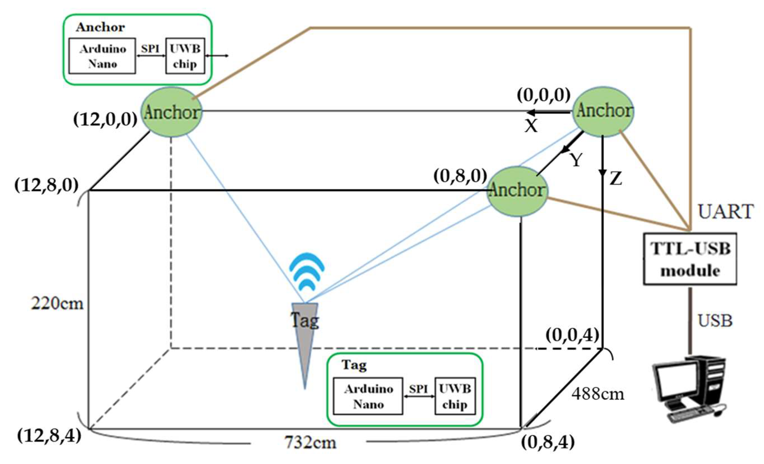
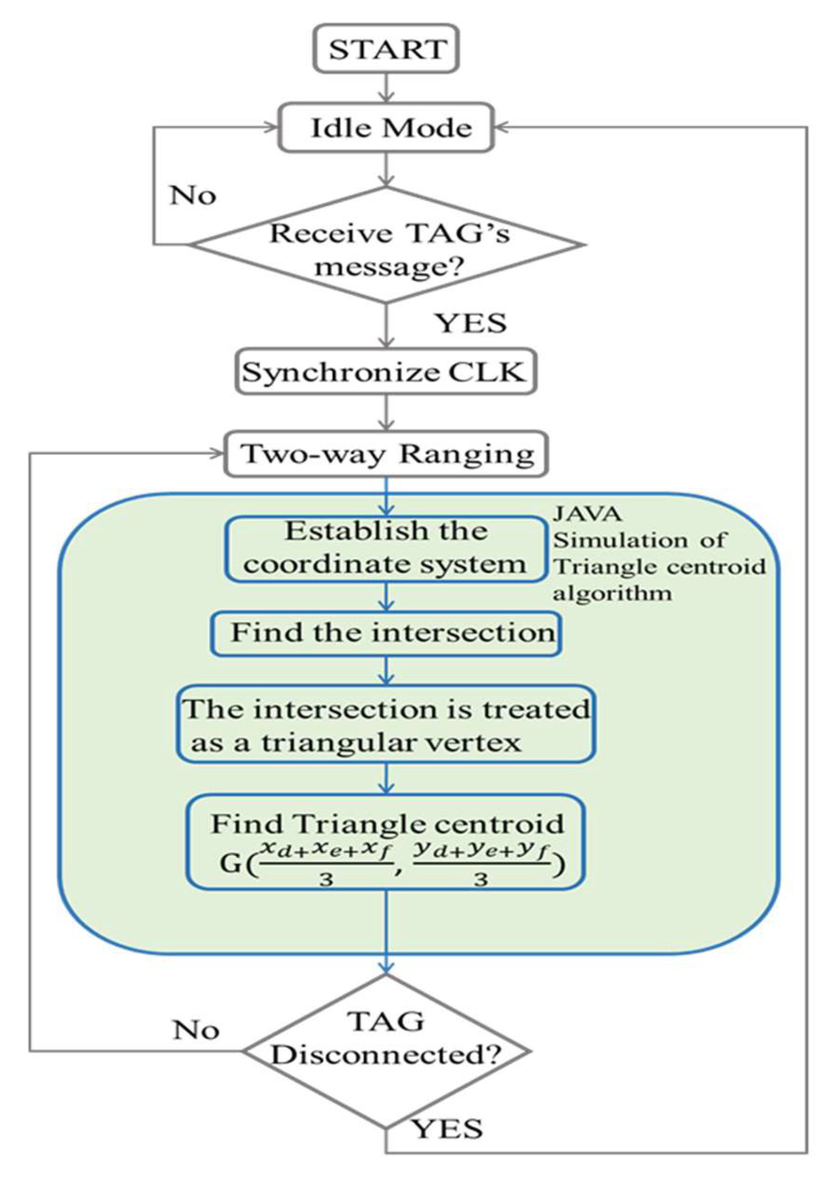
In this experiment, we conducted an indoor positioning system accuracy test in a laboratory space. As shown in Figure 1, a 3D coordinate system defined as (X, Y, Z) was established within the space. This coordinate system consists of a 12 × 8 × 4 grid, with each unit measuring 61 × 61 × 55 cm. In the figure, the green oval represents the base station (Anchor), and the gray inverted triangle represents the tag to be located (Tag). The base stations were placed in three corners of the laboratory and connected to a computer. Bilateral and bidirectional operations were then performed on the tags as described in Section 2. After measuring the distance, JAVA was used to simulate the TOA positioning method using the measured experimental values before finally measuring the positioning error through the coordinate system.

The UWB experimental module is integrated with a microprocessor and a DW1000 UWB chip manufactured by Qorvo, Inc., Greensboro, NC, USA, as shown in the illustration in Figure 1. The DW1000 UWB chip operates within a carrier frequency range of 3.5 to 6.5 GHz, supporting seven UWB channels. It transmits low-power UWB signals with a typical output power of −10.3 dBm/MHz, in compliance with FCC and ETSI emission regulations. The signal type utilizes burst position modulation (BPM) combined with binary phase shift keying (BPSK) for data encoding. The transmitted UWB pulses are extremely short, with durations of approximately 1 nanosecond, enabling precise time-of-flight (ToF) measurements and positioning accuracy of up to 10 cm. The control program in Arduino Nano is burned and the SPI bus is used to communicate with the UWB chip. Modules are divided into two types: anchor and tag according to different burning programs. The base station and the tag transmit information using ultra-wideband. In order to observe the measured distance value on the computer, the base station module uses a UART and then uses a TTL-USB. The module connects to the computer to send data to the computer.

Arduino Nano uses ATmega328 microcontroller manufactured by Microchip Technology Inc., USA, as the core of the control development board. It has 22 digital I/O ports and 8 analog I/O ports. It uses a 16 MHz crystal oscillator. It has a bootloader and does not need to be burned through other programs. Following recording, the program can be uploaded directly through the USB, so the language can be quickly compiled and implemented, and there is an open source for users to communicate. Therefore, this experiment uses Arduino Nano as the microprocessor controller to communicate with the ultra-wideband chip. Finally, the data is transmitted to the USB-STC-ISP module through UART (RS-232). The module uses a USB to connect to the computer to transmit the data to the computer.

5.2. One by One LOS Test

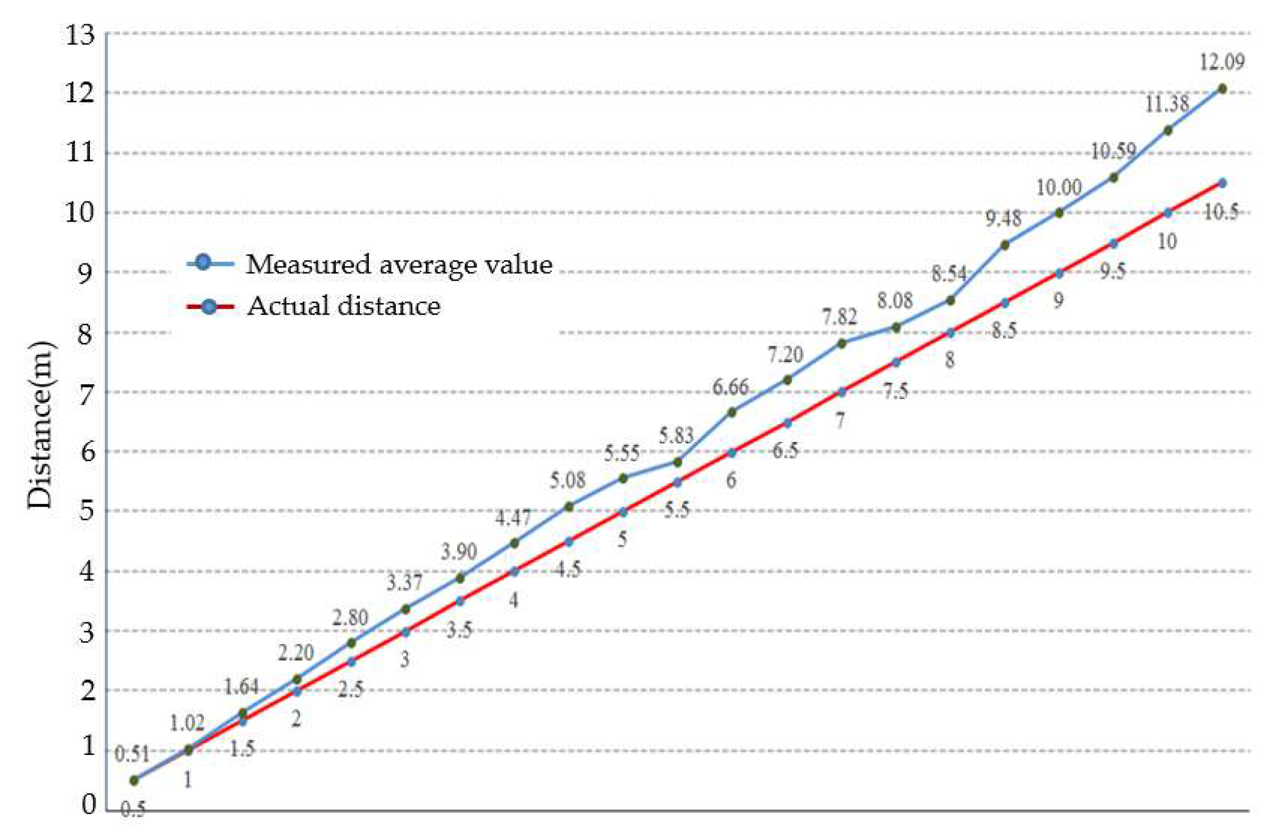
This experiment first conducts a one-to-one barrier-free distance test between devices. The actual distance is tested every 50 cm starting from 50 cm. The test results are recorded, and the average of the 30 test values is used as the test value until the actual distance is Up to 10 m, a total of 20 one-to-one barrier-free distance measurements were conducted.

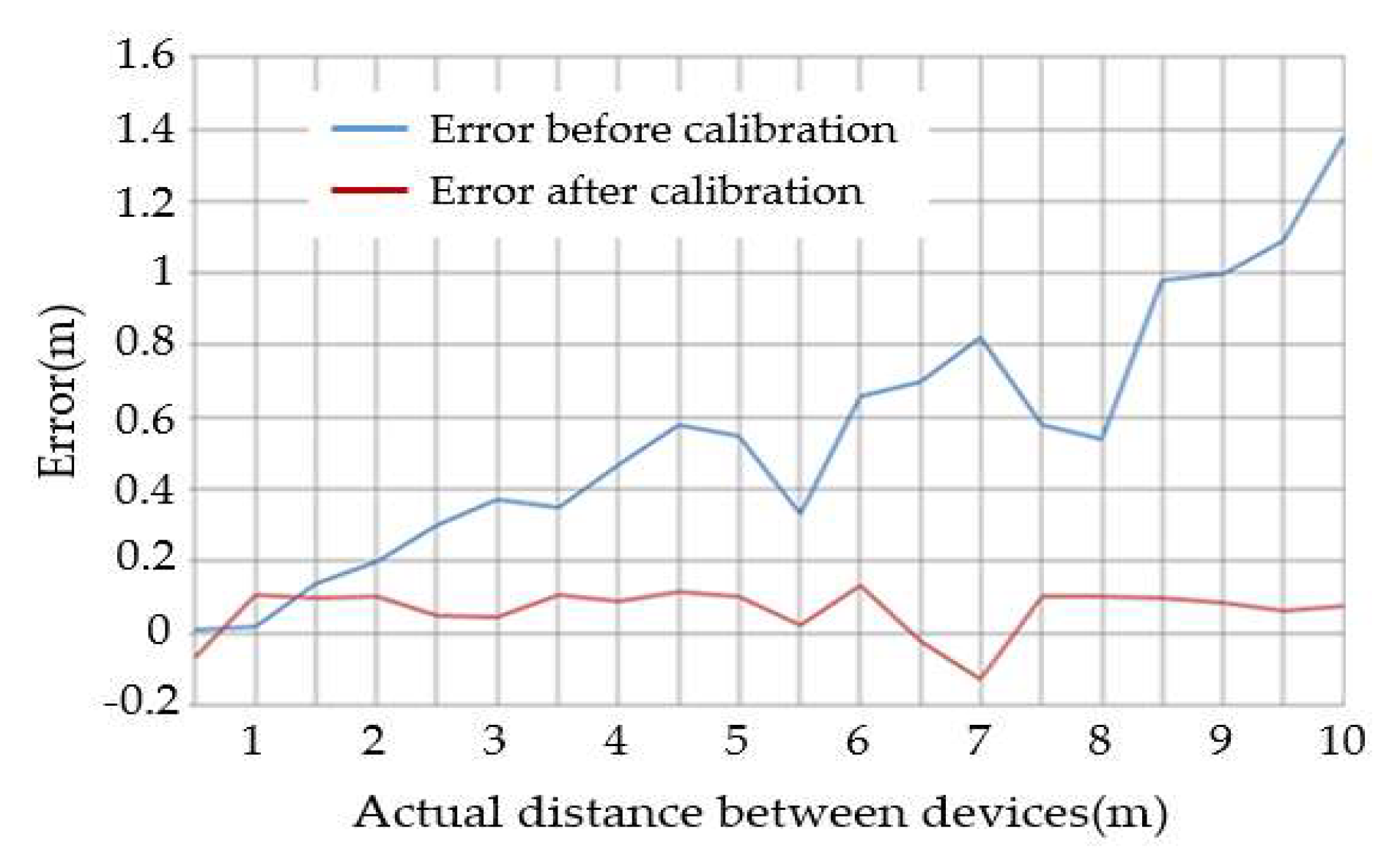
Figure 8 is the data from the one-to-one accessibility test. We conducted one-to-one distance measurements in the experimental space. We used a tape measure and floor tiles to assist in measuring the actual distance. We averaged the 30 experimental values and compared them with the actual values to calculate the error. It can be found that when the actual distance is below 6 m, the error is less than 10%, and the converted actual error value is about 20–50 cm. When the actual distance is greater than 6 m, the error distance begins to gradually increase.

Since the one-to-one distance measurement between devices will directly affect the positioning accuracy, we will correct the one-to-one distance test value and divide each section (0.50–10 m at intervals of 50 cm), taking the maximum and minimum values of 30 data points to calculate the test value, before comparing it with the actual value and find the average error value, and then use the intermediate value between the minimum value of the subsequent section and the maximum value of the previous section as the dividing point for correction.

When the actual distance is 6.50 m, the average of the 30 measured data points is 6.89 m, with a minimum value of 6.68 m, resulting in an error of 0.39 m. Meanwhile, for an actual distance of 6 m, the maximum value among the 30 measured data points is 6.39 m. Thus, the threshold point is calculated as (6.68 + 6.39)/2 = 6.54 m. This means that when the measured distance exceeds 6.54 m, an error value of 0.39 m must be subtracted to obtain the corrected measurement data.

After adding this mechanism to the program, we re-conducted a one-to-one barrier-free ranging experiment. We also conducted experiments every 50 cm starting from 50 cm, recorded the test results, and averaged the 30 test values as test value, until the actual distance is 10 m; a total of 20 one-to-one barrier-free ranging measurements are performed. As shown in Figure 9, the error value of the one-to-one distance test after correction is about 10 cm, and the accuracy has improved significantly.

5.3. TCA Localization Test

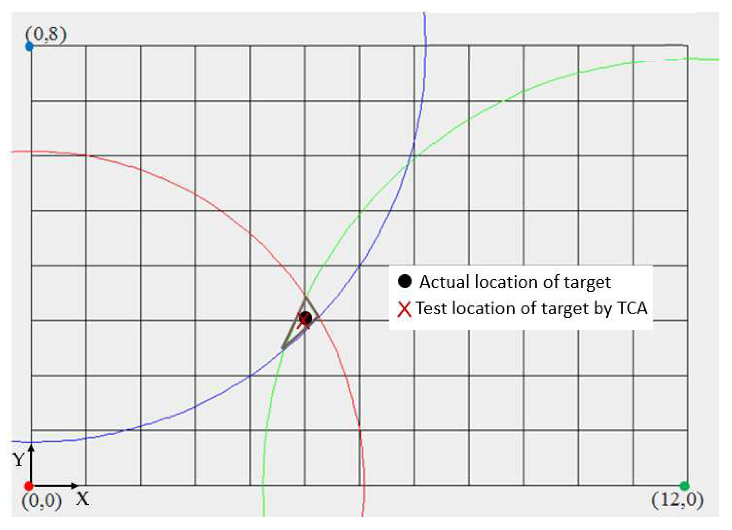
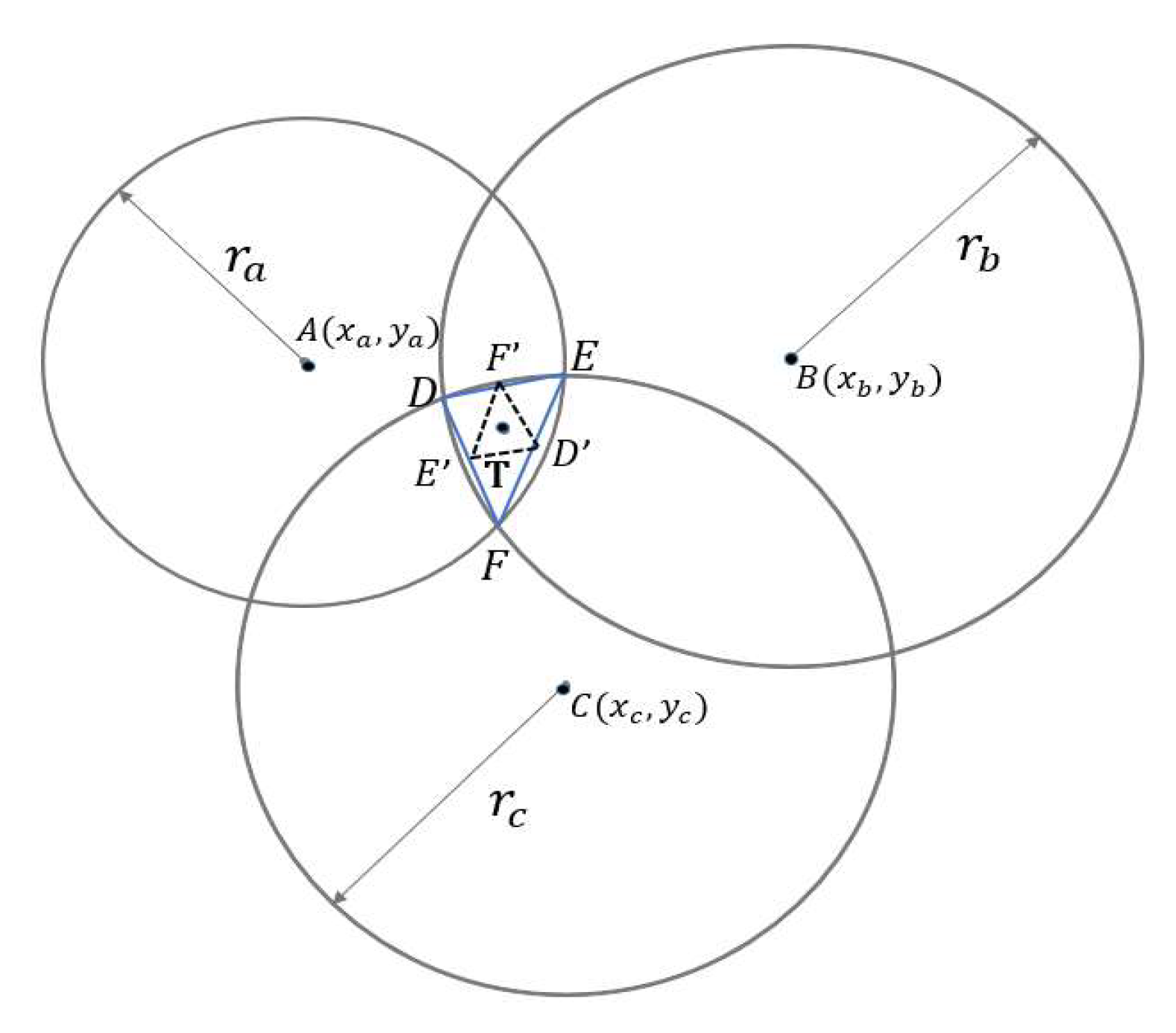
To reduce testing complexity and improve measurement accuracy, we placed the tag on the ceiling plane of the laboratory. The plane measures 732 × 488 cm, and its coordinate system (X, Y) is defined as a 12 × 8 grid, with each square measuring 61 × 61 cm. Subsequently, three base stations were placed at the origin (0, 0), on the X-axis at (12, 0), and on the Y-axis at (0, 8), as shown in Figure 10. In the figure, the black dots represent the actual positions of the tags, while the blue, red, and green dots indicate the positions of the base stations. The corresponding blue, red, and green circles are drawn using the measured distance values from each base station as the radius. The overlapping area in the center represents the region where the theoretical tag position is most likely to appear based on the TOA method. The cross mark denotes the estimated position calculated using the center of gravity positioning method.

The experimental results indicate that when the tag is closer to the origin, the intersection of the three circles can be approximately represented as a triangle. For instance, when positioning the coordinates (3, 6), the coordinates estimated using the triangle centroid algorithm are (2.73, 5.70), resulting in an actual error of approximately 24.30 cm. When positioning the coordinates (5, 3), as shown in Figure 10, the experimentally determined coordinates are (4.97, 2.99), corresponding to a positioning error of about 1.92 cm. Similarly, for the coordinates (7, 3), the calculated position is (6.78, 2.76), yielding an actual error of approximately 19.95 cm.

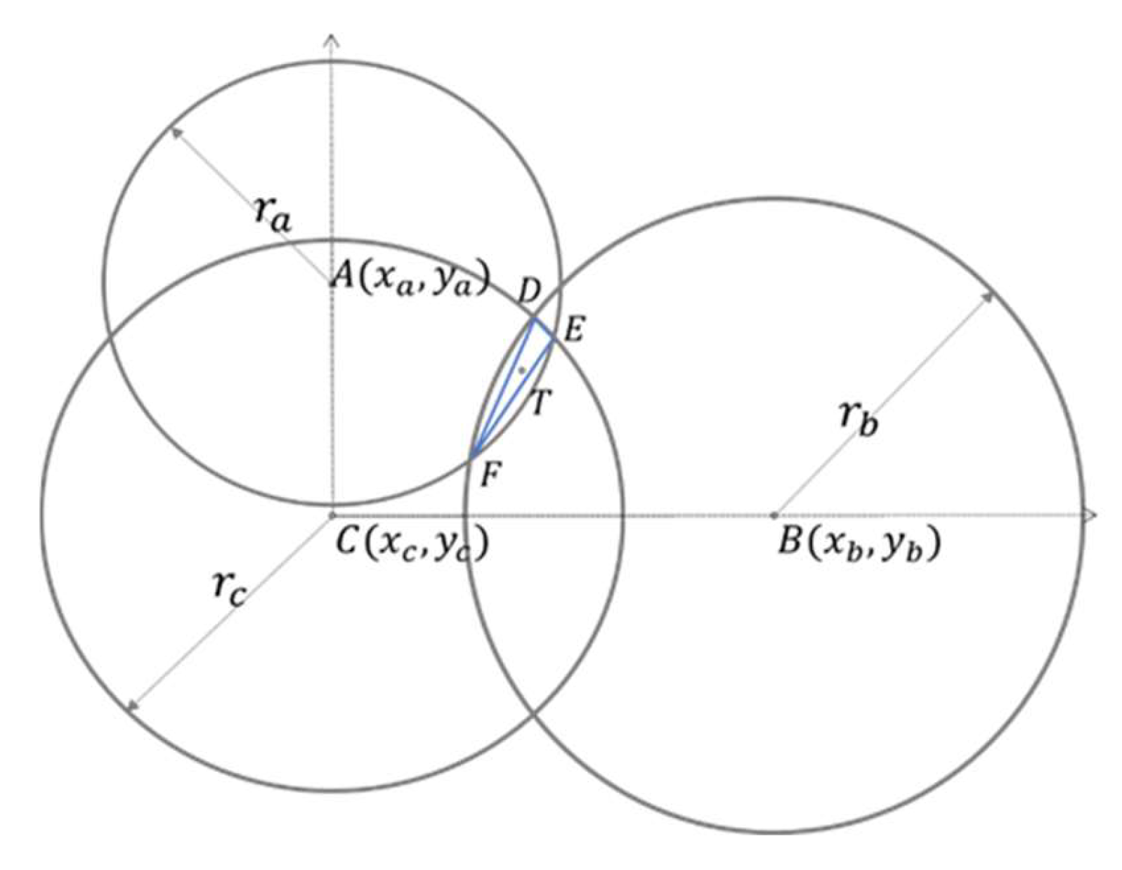
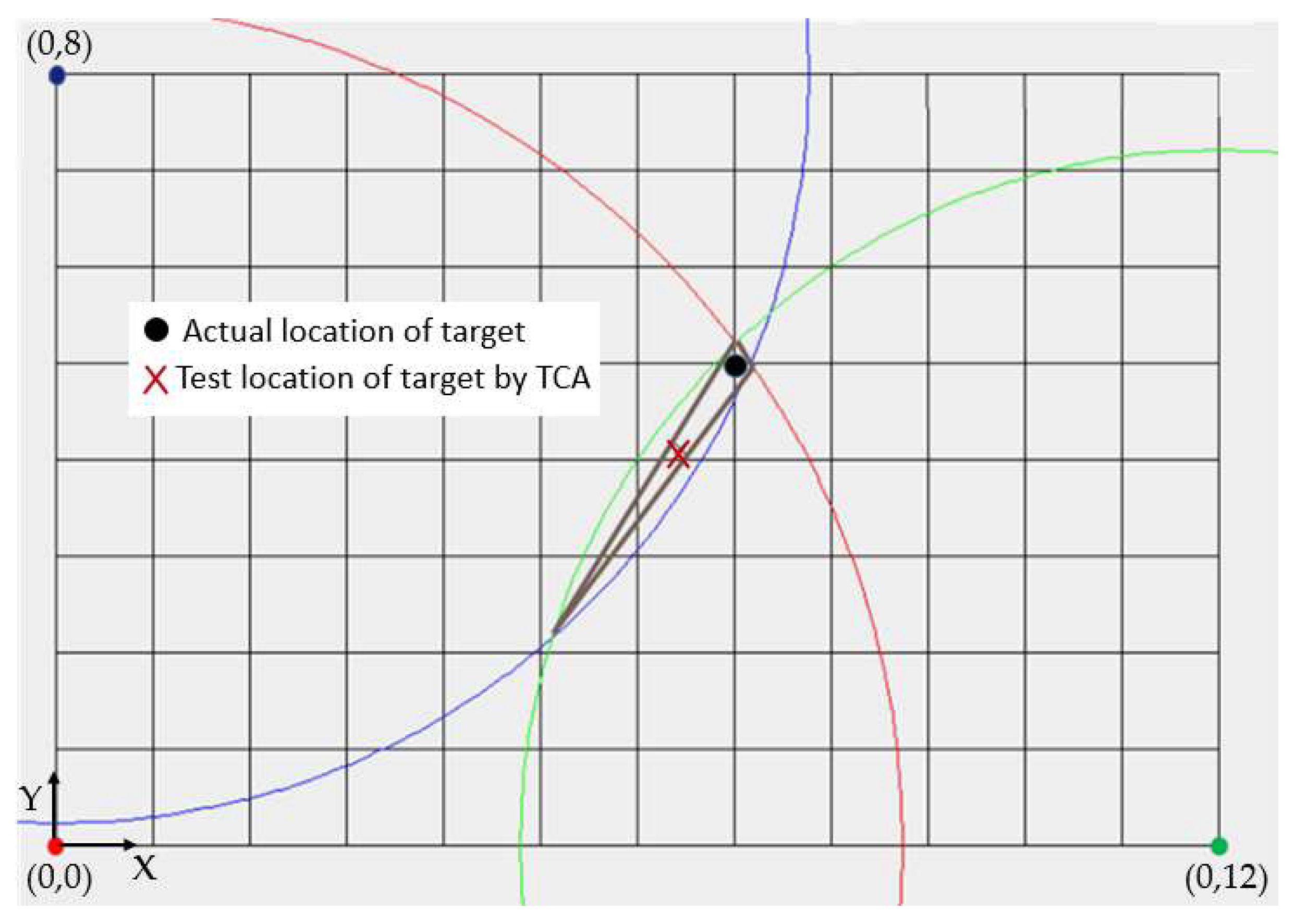
However, when the tag is placed at positions with large X and Y coordinate values—far from the origin—such as (7, 5), (10, 7), (11, 5), (0, 8), and (12, 0), the intersection area of the circles becomes elongated and narrow, making it difficult to approximate a triangular shape. For example, when positioning the coordinates (7, 5), as shown in Figure 11, the triangle centroid algorithm yields a result of (6.43, 4.12), corresponding to an actual positioning error of approximately 63.68 cm. When positioning the coordinates (10, 7), the experimentally determined coordinates are (8.34, 4.39), with an error of about 188.45 cm. Similarly, for the coordinates (11, 5), the calculated position is (9.73, 2.98), resulting in an error of approximately 145.55 cm. These results demonstrate that when both X and Y coordinate values are large, the triangle centroid algorithm becomes ineffective, leading to significant positioning errors. Detailed experimental results for 10 coordinate points within the positioning space are summarized in Table 1.

5.4. IMA Localization Test

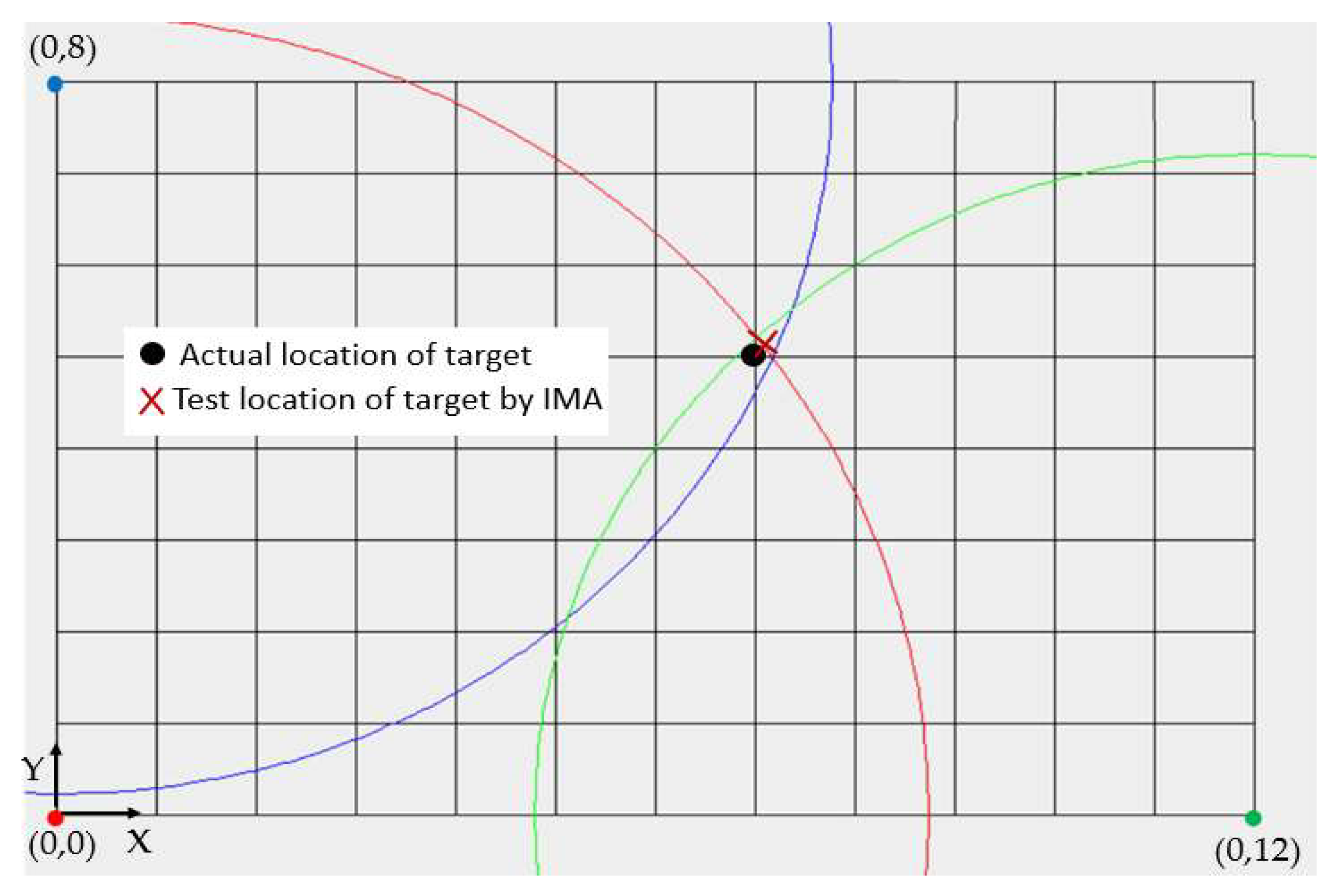
In the previous experiment of the triangle center of gravity algorithm, we found that when the label is placed with large X and Y coordinate values, that is, when it is farther away from the origin, the intersection of the three circles will become narrower and longer, and the three intersecting circles thus cannot be approximated as a triangle. If the triangle center of gravity algorithm is used to estimate the coordinates of the target object, it will be inaccurate because the triangle is too narrow and long. Therefore, we have proposed a solution to locate the intersection midpoint. As shown in Figure 12, we selected the intersection point of the red circle and the blue circle as well as the intersection point of the red circle and the green circle, and then took the midpoint as the post-positioning coordinates. This can avoid the intersection of the blue circle and the green circle. The overlapping area becomes large or narrow, and the accuracy of using the center of gravity positioning method becomes poor.

The experimental results show that when the positioning coordinates are (7, 5), the calculated positioning coordinates are (7.09, 5.10), which is converted into an actual error of about 8.57 cm; when the positioning coordinates are (10, 7), the positioning coordinates are (10.18, 7.15), and the actual error is about 14.48 cm; when positioning the coordinates (11, 5), the positioning coordinates are (11.10, 5.04), which translates into an actual error of about 6.93 cm, and there are 10 coordinate points in the positioning space. The detailed experimental results are shown in Table 1. It can be seen from the table that the positioning errors are almost all quite small, which significantly improves the positioning accuracy.

5.5. Comparison of Algorithm

After experimental testing, the triangle centroid algorithm was found to produce significant positioning errors. To further evaluate accuracy, we referred to a study published by Nantong University in China [22] and conducted a JAVA-based simulation for comparison. As illustrated in Figure 11, when targeting the coordinate (11, 5), the triangle centroid algorithm yielded a result of (9.73, 2.98), corresponding to a converted positioning error of 145.55 cm and an execution time of 17.49 μs. In contrast, the intersection midpoint algorithm proposed in this study produced a positioning result of (11.10, 5.04), with a significantly lower error of 6.93 cm and a shorter execution time of 13.65 microseconds. Similarly, the inner triangle centroid algorithm from Nantong University also achieved coordinates of (11.10, 5.04) with the same 6.93 cm error but required 33.28 μs to execute.

To calculate the standard deviation of the TCA, ITCA, and IMA errors from Table 1, the standard deviation (σ) of a dataset is given by the formula:

$$\sigma =\sqrt{{\displaystyle \frac{1}{n}}{\sum }_{i=1}^n{\left(x_i-\mu \right)}^2} ,$$

(13)

where $x_i$ represents each individual data point (i.e., localization error), μ is the average error of these data points, and n is the total number of data points. Based on Equation (13) and the error values provided in Table 1, the calculated standard deviations for the TCA, ITCA, and IMA are 72.91 cm, 3.76 cm, and 5.36 cm, respectively.

These results demonstrate that the algorithm proposed in this study offers high positioning accuracy with a simpler computation process, effectively reducing execution time. The experimental results of TCA, ITCA, and IMA positioning are shown in Table 1 below. The comparison error summarized in Table 1 is the distance between the coordinates calculated by the algorithm and the actual position of the target. A total of ten points in the coordinates were taken out for ranging experiments. The test values were simulated on the JAVA program to simulate the positioning accuracy, and the algorithm execution time was calculated. Finally, the average error and standard deviation were calculated. The optimization-based method serves as a benchmark to evaluate the trade-off between computational cost and localization accuracy. In resource-constrained systems, heuristic models such as ITCA and IMA offer a favorable balance between accuracy and computing efficiency. As demonstrated in Table 1, although ITCA achieves the highest accuracy under average error of 11.85 cm, IMA achieves a close accuracy (12.87 cm) with the shortest execution time (13.65 μs), thus offering superior performance for both computational complexity and algorithm execution time. Although the TCA performs well at certain coordinates, such as an error of 3.31 cm when positioning at (3, 1) and 1.92 cm at (5, 3). It fails to accurately locate the target when the distance from the origin increases, resulting in an average error of 75.36 cm.

Based on the algorithm time consumption shown in Table 1, the IMA proposed in this study is notably efficient, requiring only 13.65 μs to complete a positioning task. In contrast, the ITCA, reported in previous studies, is more complex and takes significantly longer, at 33.28 μs, to perform the same task. These results demonstrate that the proposed IMA not only simplifies the computational process but also achieves accurate indoor positioning with lower time consumption.

In conclusion, the TCA exhibits significant error variation; although it performs accurately at certain coordinates, the positioning error increases markedly with distance from the origin, leading to poor stability. In contrast, the ITCA shows tightly clustered and stable errors, resulting in highly consistent positioning outcomes. The proposed IMA achieves a well-balanced trade-off between computational efficiency and positioning accuracy, making it particularly suitable for real-time indoor localization applications.

6. Conclusions

This study presents a comparative analysis of indoor positioning algorithms using UWB technology, with a focus on improving accuracy and computational efficiency. The proposed intersection midpoint algorithm demonstrates notable advantages in both precision and execution speed. While the traditional triangle centroid algorithm performs adequately near the origin, its accuracy degrades significantly as the target moves farther away. The inner triangle centroid algorithm from Nantong University achieves the highest accuracy with an average error of 11.85 cm but requires a longer execution time of 33.28 μs. In contrast, the intersection midpoint algorithm achieves a comparable average error of 12.87 cm with a faster execution time of just 13.65 μs. These results confirm that the intersection midpoint method offers an effective balance between computational simplicity and positioning accuracy. This makes it especially suitable for real-time indoor applications where low latency and precision are critical, such as in healthcare monitoring and smart building navigation systems.