Abstract
The COVID-19 pandemic has presented significant challenges to global healthcare, bringing out the urgent need for reliable diagnostic tools. Computed Tomography (CT) scans have proven instrumental in detecting COVID-19-induced lung abnormalities. This study introduces Convolutional Neural Network, Graph Neural Network, and Vision Transformer (ViTGNN), an advanced hybrid model designed to enhance SARS-CoV-2 detection by combining Graph Neural Networks (GNNs) for feature extraction with Vision Transformers (ViTs) for classification. Using the strength of CNN and GNN to capture complex relational structures and the ViT capacity to classify global contexts, ViTGNN achieves a comprehensive representation of CT scan data. The model was evaluated on a SARS-CoV-2 CT scan dataset, demonstrating superior performance across all metrics compared to baseline models. The model achieved an accuracy of 95.98%, precision of 96.07%, recall of 96.01%, F1-score of 95.98%, and AUC of 98.69%, outperforming existing approaches. These results indicate that ViTGNN is an effective diagnostic tool that can be applied beyond COVID-19 detection to other medical imaging tasks.
1. Introduction
The COVID-19 pandemic has had a profound impact on healthcare systems around the world and emphasizes the urgent need for effective, rapid, and reliable diagnostic tools. Traditionally, Real-Time Polymerase Chain Reaction (RT-PCR) has been the primary method for detecting SARS-CoV-2 infection. However, despite being the gold standard, RT-PCR has notable limitations: It is time-consuming, prone to false negatives, and highly dependent on the quality of the sample and the timing of collection. This has led to an increasing interest in alternative diagnostic methods that can offer faster and potentially more reliable results, especially in clinical settings of high demand [1,2].
Computed Tomography (CT) imaging has emerged as a promising complementary diagnostic tool for COVID-19, primarily due to its high sensitivity in detecting COVID-19 related lung abnormalities such as ground-glass opacities, septal thickening, and consolidations. Unlike RT-PCR, which directly detects viral genetic material, CT imaging provides a visual representation of disease progression, capturing structural changes in lung tissue. Studies have shown that CT scans can reveal abnormalities even in cases with low viral load where RT-PCR might yield a false negative, making CT a valuable tool for timely and accurate diagnosis [3,4,5].
The application of artificial intelligence (AI), particularly deep learning, has transformed medical imaging by enabling automated analysis and interpretation of complex visual data. Convolutional Neural Networks (CNNs) have been widely adopted for image analysis and have demonstrated considerable success in detecting lung abnormalities associated with COVID-19. However, CNNs have limitations when it comes to capturing complex spatial dependencies in an image, which are crucial for understanding nuanced patterns in medical imaging [6]. Vision Transformers (ViTs), which leverage self-attention mechanisms, offer a solution by modeling global dependencies across an image, allowing them to identify broader patterns that may indicate the presence of COVID-19. Despite their strengths, ViTs can sometimes overlook local structural relationships, which are essential to detect fine-grained features in medical images, such as small lesions or subtle tissue changes specific to COVID-19.
Several research studies have explored the application of Graph Neural Networks (GNNs) and Vision Transformers (ViTs) in medical imaging and classification tasks; however, no existing research has explicitly combined GNNs and ViTs for SARS detection. GNNs are effective in capturing spatial and topological relationships within the data, making them suitable for structural pattern recognition in images. For instance, ClusterViG combined CNNs with GNNs for improved feature representation [7]. On the other hand, ViTs have shown strong performance in medical imaging, especially in the classification of COVID-19 using chest CT scans [8], and researchers have also investigated the impact of different patch sizes in ViTs for the classification of lung diseases, highlighting their ability to model global dependencies in image analysis [9].
Existing SARS-CoV-2 detection frameworks predominantly rely on CNN-based deep learning models or ViTs independently without leveraging GNNs for spatial and relational inference. This suggests that a Vision Transformer and Graph Neural Network (ViTGNN) architecture could introduce a novel and effective method to improve the diagnostic accuracy of SARS-CoV-2 detection from CT scans. The rationale behind the combination of ViT and GNN (ViTGNN) is based on their complementary strengths. The GNN captures relationships and structural patterns in data [10], while the ViT excels at processing visual information [11,12]. This hybrid process allows ViTGNN to overcome the individual limitations of CNNs and ViTs [13], offering a more comprehensive approach to the diagnosis of COVID-19. The key contributions of this paper are as follows.
- We develop ViTGNN, a hybrid model that uses a GNN for feature extraction and a ViT for classification to improve the detection of SARS-CoV-2 in CT scans.
- We enhance image representation using advanced preprocessing techniques such as CLAHE, Gaussian blurring, and data augmentation on COVID-19 and non-COVID-19 CT scan images.
- We train and optimize ViTGNN on a dataset in order to ensure generalization across unseen data.
- We evaluate ViTGNN performance against multiple baseline models using accuracy, precision, recall, F1-score, and AUC.
This paper is organized as follows: Section 2 provides a review of related work. Section 3 describes the materials and methods employed in the study. Section 4 presents the experimental results along with a comprehensive discussion. Section 5 concludes the paper by summarizing the key findings. Finally, Section 6 discusses the study limitations and outlines potential directions for future research.
2. Related Works
In this section, we present the frameworks and algorithms pertinent to our study. This review of the literature focuses on the application of artificial intelligence, such as deep learning and machine learning, in the detection of COVID-19, with an emphasis on their roles in the processing and analysis of image datasets.
Recently, wavelet-based super-resolution methods have gained attention for their ability to enhance fine-grained image features, which can be crucial for improving downstream medical diagnostic tasks. For instance, Yu et al. [14] proposed a wavelet pyramid recursive neural network (WPRNN) constrained by wavelet energy entropy, which fuses both shallow and deep wavelet coefficient features across multiple resolutions to reconstruct high-quality medical images. This approach not only improves perceptual reconstruction quality but also preserves subtle structural details critical for accurate interpretation.
Parikh et al. [7] proposed ClusterViG, a vision GNN that improves efficiency with Dynamic Efficient Graph Convolution (DEGC) by partitioning images, parallelizing graph construction, and integrating local–global feature learning. Additionally, it optimizes k-NN graph construction and enhances context awareness using GATv2. The results demonstrate 87.2% top-1 accuracy in ImageNet-1K, improved object detection and segmentation in MS COCO 2017, and up to 5× faster inference, making ClusterViG highly efficient and scalable for vision tasks. A transformer-based COVID-19 diagnosis framework that uses UNet for lung segmentation and Swin Transformer for classification was introduced by Zhang et al. [15]. Evaluated on MIA-COV19D, Swin Transformer achieved an F1-score of 0.935 (validation) and 0.84 (test), outperforming BiT-M and EfficientNetV2, with the latter excelling in precision (93.7%).
TransGNN was proposed, a hybrid Transformer–GNN model for recommender systems that alternates Transformer and GNN layers to expand the receptive field while preserving structural information. Attention sampling, positional encoding, and efficient sample updates enhance efficiency and scalability. The model was evaluated on Yelp, Gowalla, Tmall, Amazon-Book, and MovieLens. TransGNN outperforms GNN and Transformer baselines, achieving up to 21.04% improvement in Recall@20 while reducing computational complexity, demonstrating its effectiveness and scalability in recommendation systems [16]. Shome et al. [17] presented COVID-Transformer, a ViT-based model for COVID-19 detection using a 30K-image dataset (COVID-19, normal, pneumonia). It was trained with the NovoGrad optimizer and achieved 98% accuracy (AUC 99%) for binary and 92% accuracy (AUC 98%) for multi-class classification, outperforming CNN models. That is, Grad-CAM visualizations enhance interpretability for diagnosis.
In the study in [9], Vision Transformers (ViTs) were evaluated for COVID-19 and diseased lung classification using Iran’s COVID-19 CT dataset (377 patients) and Malaysia’s dataset (81 diseased, 15 normal cases), where 32 × 32 patches achieved the highest accuracy (95.36%), while larger patches reduced performance. ViT outperformed CNN models (ResNet50, Xception) in efficiency, demonstrating its potential in medical imaging. Wang et al. [4] introduced Contrastive Cross-Site Learning with Redesigned COVID-Net for COVID-19 CT classification, addressing domain shifts in multi-site datasets. The datasets include SARS-CoV-2 (2482 CT images) and COVID-CT (349 CT images), which incorporated domain-specific batch normalization and contrastive learning for feature extraction. The model achieved 96.24% AUC, 92.1% accuracy, 91.3% sensitivity, and 93.2% precision on SARS-CoV-2, and 85.32% AUC, 84.5% accuracy, 83.7% sensitivity, and 85.9% precision on COVID-CT. It outperforms standard COVID-Net by 12.16% and 14.23% in AUC and surpasses state-of-the-art multisite learning methods.
Xiao et al. [18] presented TCGN, a Transformer-CNN-GNN model for gene expression prediction from histopathological images. It processes single-spot images, integrating a CNN for local features, a Transformer for global learning, and a GNN for cell organization analysis, which enhances interpretability. The model was evaluated on HER2+ (32 sections, eight patients), cSCC (12 sections, four patients), and spatialLIBD (59,904 spots, 20 sections, 3 donors). TCGN achieves the highest median PCC (0.232), outperforming ST-Net, HisToGene, and Hist2ST with fewer parameters (86.24M) and lower GPU memory.
Choi et al. [19] proposed ICEv2, an interpretable method that assigns class-relevance probabilities to individual patches using adversarial normalization, circumventing the limitations of traditional attention-based visualizations. ICEv2 identifies foreground (task-relevant) and background patches without modifying the model’s architecture or retraining weights. The method produces fine-grained visual saliency by interpreting output logits at the patch level rather than relying on [CLS] token contributions. Applied to segmentation datasets, ICEv2 demonstrated strong performance in visual localization, offering a viable pathway for producing trustworthy visual explanations in healthcare settings.
Marchetti et al. [20] addressed ViT inefficiencies by introducing Token Reduction via an Attention-Based Multilayer Network (TRAM). TRAM constructs a graph from multilayer attention matrices and computes centrality scores to prune less informative tokens at each transformer layer. Unlike methods that rely on [CLS] tokens or retraining, TRAM performs static, architecture-agnostic pruning, which maintains classification performance while substantially reducing memory usage and inference time. These characteristics are highly desirable in real-time or embedded diagnostic systems, where latency and resource consumption are constrained.
Englebert et al. [21] developed Transformer Input Sampling (TIS), a saliency technique that avoids the artifact generation associated with conventional perturbation-based methods, such as RISE or Score-CAM. TIS leverages the inherent flexibility of ViTs to handle variable-length token sequences, enabling interpretability by selectively omitting tokens post-embedding and measuring their impact on class predictions. Sampling embedded token subsets and assessing prediction shifts, TIS constructs faithful, class-specific saliency maps without corrupting the input image. This strategy ensures the generation of clinically meaningful explanations, which is essential for radiological review in COVID-19 diagnosis.
Artificial intelligence (AI) and deep learning (DL) have transformed CT-based diagnostics, allowing automated analysis and interpretation of intricate visual data. Convolutional Neural Networks (CNNs), widely used in medical imaging, have effectively captured long-range dependencies and complex spatial relationships across an image in detecting localized lung abnormalities associated with COVID-19 [22]. However, CNNs have limits, and Vision Transformers (ViTs), which use self-attention mechanisms to identify global patterns, offer an alternative by modeling image-wide dependencies. This global perspective enables ViTs to detect broader image patterns but can sometimes overlook local structural details essential for clinical precision [23].
To address these limitations, hybrid models that combine CNNs, ViTs, and Graph Neural Networks (GNNs) have gained attention. GNNs focus on relational data within images, representing patches as nodes and spatial relationships as edges, which is crucial for capturing local details. Nguyen et al. showed that incorporating spatial information through a GNN could improve diagnostic accuracy, supporting the potential of hybrid models for the detection of COVID-19 in CT imaging [24].
As summarized in Table 1, a wide range of deep learning approaches have been proposed for COVID-19 detection using chest CT and X-ray images. These methods vary significantly in terms of datasets used, network architectures, and reported performance. For instance, some models, such as Deep CNN [25] and COVID-Net [26], focus on conventional CNN architectures. In contrast, others incorporate more advanced designs, such as 3D CNNs [27], residual attention mechanisms [28], or hybrid ensembles, like Xception with ResNet50V2 [29]. Moreover, studies also differ in the imaging modality used either CT scans or X-rays and in their learning strategies, including weakly supervised learning [30], GAN-based augmentation [31], and radiological descriptive analysis [32]. These variations lead to a wide range of performance metrics, with accuracy values spanning from approximately 85% to over 99%, depending on task complexity, class balance, and dataset scale.

Table 1.
Comparative Summary of Related Deep Learning Models for COVID-19 Detection.
3. Materials and Methods
3.1. Data Preprocessing
The SARS-CoV-2 CT Scan dataset, Figure 1, is publicly available on Kaggle. It consists of 1252 CT scans from patients diagnosed with SARS-CoV-2 infection (COVID-19) and 1230 scans from non-infected individuals, resulting in 2482 CT scans. Data were collected from actual patients in hospitals in São Paulo, Brazil [22]. In the context of COVID-19 image analysis, pre-processing techniques are important to enhance image quality, improve feature extraction, and increase the accuracy of machine learning and deep learning models.
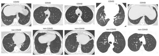
Figure 1.
Sample images of SARS-CoV-2 in CT scans.
Here, we explain the specific image preprocessing methods used in this study to enhance the quality of the training data. A total of 1986 CT scans were used, comprising COVID-19 and non-COVID-19 cases, to train the model representing 80% of the complete dataset (2482 scans). The preprocessing steps included the following.
3.1.1. Contrast-Limited Adaptive Histogram Equalization (CLAHE)
CLAHE is an advanced local contrast enhancement technique that improves the visibility of features in low-contrast images [41]. In this study, CLAHE was applied using Python 3.11.7 library OpenCV (4.11.0 version) via the functions cv2.createCLAHE() and cv2.cvtColor(). The image was first converted from the BGR (Blue, Green, Red) color space to the YUV (Luminance, Chrominance) color space, allowing contrast enhancement to be applied specifically to the luminance (Y) channel. Previous research [42] demonstrated that applying CLAHE to fundus images significantly improved feature visibility and enhanced the classification performance of deep learning models such as VGG16 and EfficientNetB4.
3.1.2. Gaussian Blur
Gaussian blur is a widely used image processing technique to reduce noise and fine detail by convolving the input image with a Gaussian kernel. This method produces a smoothed version of the image in which each pixel value is replaced by a weighted average of its surrounding pixels, where the weights decrease with increasing distance from the center pixel [43]. In this work, we implemented Gaussian blur using the OpenCV function cv2.GaussianBlur(), which applied a 5 × 5 Gaussian kernel with an automatically computed standard deviation. The 5 × 5 kernel operates over a 25-pixel neighborhood, performing a weighted average in which the center pixel contributes most strongly. This effectively reduces noise while preserving the overall image structure.
3.1.3. Data Augmentation
To improve the generalization of the model in the unseen dataset and reduce the risk of overfitting, a set of data augmentation techniques was applied to the training dataset. These included random resized cropping, horizontal flipping, affine rotation, color jittering, and channel-wise normalization. Random resized cropping was used to simulate variations in object scale and spatial position, while horizontal flipping introduced invariance to image orientation. A random rotation of up to ±15 degrees addressed minor angular deviations commonly found in real-world scenarios. Photometric transformations were incorporated via brightness and contrast adjustments using color jittering, mimicking diverse lighting conditions. Finally, normalization was applied to standardize the pixel value distributions across image channels, facilitating stable and efficient model training. As highlighted in the work in [44], such geometric and photometric augmentation strategies are foundational to modern preprocessing pipelines, offering an efficient means of increasing both the diversity and realism of training data without compromising semantic integrity.
3.2. Evaluation Metrics
The performance of the ViTGNN model for detecting COVID-19 from CT scans is evaluated using key performance indicators, including accuracy, precision, recall, F1-score, and Area Under the Curve (AUC). These metrics provide a comprehensive evaluation of the ability of the model to accurately classify patients as COVID-positive or COVID-negative. The evaluation depends on components that include True Positives (TPs), True Negatives (TNs), False Positives (FPs), and False Negatives (FNs), which offer insight into the effectiveness of the model in distinguishing between COVID-19 and non-COVID-19 cases. These components ensure a thorough evaluation of ViTGNN diagnostic performance.
3.3. Experimental Setup
The experimental setup evaluated the performance of the ViTGNN framework for detecting SARS-CoV-2 from CT scan images. The dataset was divided into training, validation, and test sets (80:10:10). ViTGNN used Convolutional Neural Networks (CNNs) and Graph Neural Networks (GNNs) to extract graph-based features from CT scans, which were then processed by Vision Transformers (ViT) for high-level feature classification. This hybrid approach ensured that the model leveraged the strengths of both architectures for improved diagnostic accuracy. Training was carried out on a system with the following specifications: 128.0 GiB memory, an AMD Ryzen Threadripper 3960X 24-core processor × 48, NVIDIA Corporation GA102 [GeForce RTX 3090] graphics, 2.9 TB disk capacity, Ubuntu 22.04.5 LTS (64-bit) operating system, and GNOME version 42.9.
The training environment used the Adam optimizer with a learning rate of 0.0001. The model was trained for 50 epochs with a batch size of 32, incorporating early stopping to prevent overfitting. Image preprocessing techniques such as CLAHE, Gaussian blurring, and image augmentation enhance image quality and improve feature detection. The implementation was carried out using PyTorch v2.6.0 and PyTorch Lightning v2.3.1, with additional libraries such as NumPy v1.26.4, Pandas v2.2.1, and Matplotlib v3.8.3. ViTGNN performance was assessed using key metrics such as accuracy, precision, recall, F1-score, and AUC. The results demonstrate the ability of the model to effectively detect SARS-CoV-2 from CT scans, highlighting its potential for medical diagnostics and its broader applicability to other healthcare challenges involving complex imaging data.
3.4. Implementation
The ViTGNN architecture is a hybrid model that combines Convolutional Neural Networks (CNNs), Graph Neural Networks (GNNs), and Vision Transformers (ViTs) to make use of their strengths in image analysis. The architecture captures both local and global features as well as structured relational information within an image. CNNs are good at extracting low-level and mid-level visual features such as edges, textures, and shapes through localized reception, but CNNs struggle to model long-range dependencies and relationships [45,46]. GNNs introduce a graph-based representation that can model spatial relationships or other structured connections between image regions, addressing the limitation that CNN feature maps alone do not explicitly encode higher-level topological relations [10,46]. Although ViT, on the other hand, uses self-attention to capture global context and long-range interaction across an entire image, pure ViT models can miss local details without a large training dataset [11,12,45].
The integration of these three components, called ViTGNN, as shown in Figure 2, is specifically designed to improve the detection of SARS-CoV-2 in CT scans, which aims to explore CNNs for hierarchical local feature extraction, GNNs for spatially structured feature refinement, and ViTs for global feature interaction and classification. This synergy addresses the shortcomings of using each network type in isolation, and information passed through these stages can achieve a more effective representation and detection of COVID-19 and non-COVID-19 cases. The following sections detail each component and its integration with ViTGNN.
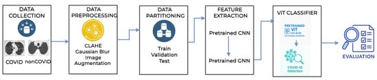
Figure 2.
Architecture model of the proposed ViTGNN framework.
3.5. CNN Feature Extractor
The first component is the Convolutional Neural Network feature extractor, where the CNN model is trained to learn spatial features like edges and textures from the preprocessed images (128 * 128 images—each image has a width of 128 pixels and a height of 128 pixels). The CNN architecture is designed similarly to classic models such as VGG or ResNet, and comprises two convolutional layers comprising batch normalization, ReLU activation, dropout for regularization, and global average pooling to aggregate the extracted features. That is, the first convolutional layer (conv1) applies a 3 × 3 filter with 32 filters, extracting basic features like edges, and the second layer (conv2) uses a 3 × 3 filter, but with 64 filters, to capture more complex patterns for better feature representation in the COVID-19 and non-COVID-19 cases. Batch normalization is used after convolutional layers to stabilize and speed training by normalizing the activation, while Dropout is used to regularize fully connected layers. However, in traditional CNN, it is common to use dropouts toward the end of the network rather than between convolutional layers. The final CNN layer (before the GNN module) outputs a feature map of size H×W with D feature channels; this can be thought of as a set of D-dimensional feature vectors arranged on a 2D grid corresponding to different image locations.
In summary, the CNN provides a rich, low-dimensional image representation that retains essential spatial information. Transforming raw pixels into feature vectors that encode local patterns, the CNN performs feature extraction and dimensionality reduction, making subsequent processing easier.
3.6. GNN-Based Spatial Representation Module
After the CNN, the output incorporates a Graph Neural Network module to take advantage of a graph-based representation of the features of the image. The motivation for this step is that treating the image as a graph of regions allows the model to explicitly reason about spatial relationships and context in a way that a regular CNN cannot [46]. In the CNN feature map, each cell (spatial location) is independent beyond the localized receptive field captured by convolution; by building a graph, we can connect distant regions or enforce longer-range interactions through message passing. This helps capture topological and relational information; for example, parts of an object can be connected on the graph to ensure that their features influence each other’s representation.
3.6.1. Graph Construction
We construct a graph , where each node represents a spatial region in the CNN feature map. Each node is initialized with a feature vector extracted from the CNN at its corresponding location. Given a CNN-generated feature map of size , the graph consists of nodes, where each node is associated with a D-dimensional feature vector. The edge set E defines the connectivity between nodes according to spatial adjacency, and each node is connected to its immediate neighbors in a four-connected grid structure, linking to adjacent nodes in the left, right, top, and bottom directions. This was implemented using relative coordinate offset neighbors = [(−1, 0), (1, 0), (0, −1), (0, 1)] that represent the top, bottom, left, and right neighbors, respectively. That is, only neighbors that fall within the valid spatial boundaries of the feature map are included in the graph. The grid-based graph structure preserves the spatial relationships in the CNN feature map, facilitating information propagation through the GCN. The 2D grid connectivity is computationally efficient and is well-suited for structured feature extraction from medical images. In addition, self-loops are included, which allow each node to retain its feature information during the Graph Convolutional Network (GCN) aggregation process. This helps stabilize the model by preserving local feature representations. That is, the self-loop is an edge that connects a node to itself.
3.6.2. GCN Architecture
With the graph defined, we apply a Graph Convolutional Network (GCN) to refine the node features. The GCN propagates information across these connections through message passing, where each node updates its feature representation by aggregating information from its neighbors. The GCN in our implemented model consists of two graph convolutional layers, which sequentially update the node features. The first GCN layer transforms the initial node features, while the second layer further refines these representations. Mathematically, the update of the feature for a node i is defined as
where:
- represents the set of neighboring nodes connected to node i.
- is a normalization factor based on the degrees of the nodes to ensure numerical stability.
- is a learnable weight matrix that applies a linear transformation to the features.
- is a non-linear activation function (ReLU).
Each GCN layer in our model follows three key steps.
- Linear transformation, where we project the feature vectors of the nodes into a new feature space using .
- Neighborhood aggregation, where we sum the transformed features of neighboring nodes using the adjacency matrix.
- Nonlinearity, where we use a Rectified Linear Unit (ReLU) activation function to add complexity to the feature representations. To avoid overfitting, we add dropout regularization after each GCN layer.
3.6.3. Node Feature Updates and Message Passing
The two-layer GCN architecture allows information to propagate beyond immediate neighbors. Each node aggregates features from its direct one-hop neighbors in the first layer. In contrast, in the second layer, each node incorporates information from its two-hop neighborhood, allowing our model to learn more contextual representations while preserving local spatial relationships. The GCN output retains the graph structure but contains refined node embeddings that integrate information from the surrounding regions. After graph convolution, we reshape the output node features into a 2D feature map to ensure compatibility with the Vision Transformer (ViT) for final classification. Unlike more complex graph-based architectures, such as Graph Attention Networks (GATs), which assign different importance to neighbor nodes, the GCN in our model applies uniform neighborhood aggregation, making it computationally efficient while capturing local dependencies in the image. In structuring the graph with spatial adjacency, we maintain the hierarchical feature representation obtained from the CNN while allowing information to flow across spatially connected nodes. The refined features provide a better representation of the image data before being processed by ViT for classification.
The GNN module adds a relational inductive bias. That is, it forces feature propagation in ways that reflect image topology, which can improve the learned representation for the subsequent classifier. CNNs model local patterns well but fail to capture long-range or topological relations. In contrast, GCNs easily capture contextual relationships, combining them and incorporating local features and long-distance dependencies [46].
In summary, the proposed framework uses a staged pre-training approach for feature extraction (Figure 1). In Stage 1, a CNN is pre-trained on the whole training set to extract localized visual features from the CT scan. The CNN comprises convolutional blocks with ReLU activations, batch normalization, and max-pooling, followed by dense layers used only during pre-training. Once trained, the convolutional layers serve as a fixed feature extractor, and their output feature maps are retained for use in downstream applications. In Stage 2, these feature maps are converted into a grid-structured graph where each spatial region corresponds to a node and edges encode local spatial adjacency. A Graph Convolutional Network is then applied to propagate contextual information across the graph. This integration allows the GCN to operate on rich, pre-trained local features, enabling the model to learn both local and global representations for robust downstream classification.
3.7. Vision Transformer (ViT) Classifier
The final stage of the model is a Vision Transformer (ViT) that serves as the classifier. The ViT takes the set of node features output by the GNN and processes them with a self-attention-based transformer encoder to produce a classification. In practice, the GNN output (the graph node features) is converted into a sequence of vectors suitable for transformer input. This involves flattening the graph node feature matrix into a sequence of length N (where N is the number of graph nodes, e.g., if using a grid graph). Each of these N feature vectors acts as a token or patch embedding for the transformer [47,48]. Before data is fed into the transformer, a learned positional encoding is added to each token. Unlike the CNN feature map, which has an implicit positional structure by its index, and the graph, which has an inherent structure, the transformer self-attention mechanism lacks an inherent sense of position. If the graph is a regular grid, 2D positional encodings can be flattened to align with the sequence. For simplicity, one can also flatten in row-major order and use a 1D positional embedding of length N. This positional information helps the ViT distinguish spatial relationships, allowing it to differentiate. We adopt a Vision Transformer encoder for classification, which consists of multiple layers of multi-head self-attention and feedforward networks with skip connections. A special classification token (CLS token) is added to the sequence, a learned embedding vector that does not correspond to a specific image patch but serves as an aggregate representation. The sequence length entering the transformer becomes (the N node features plus the CLS token). The self-attention mechanism of the transformer enables each token to attend to the content of the features of each other, allowing the model to focus on the relevant regions for classification.
For instance, if combinations of distant regions are important for a class, the self-attention layers capture these interactions, something neither the CNN nor the local GNN neighborhood fully captures. Multi-head attention enables the model to attend to multiple patterns or relationships in parallel, with each attention head learning a distinct attention map. The output of each attention layer is processed through a feedforward network and normalization, following the standard transformer architecture. During forward propagation, self-attention computes attention weights between every pair of tokens based on the products of their projected feature vectors. This results in a globally aware feature update, where each token receives a weighted sum of all other tokens’ features. Consequently, the transformer output features encode global dependencies, with the representation of the CLS token at the final layer serving as an aggregated image descriptor that has attended to various important regions of the image, and CLS token output is then fed to a classification head.
3.8. Integration of CNN-GNN-ViT
Integrating CNN, GNN, and ViT into a unified model called ViTGNN involves structuring the data flow and potentially training in multiple stages. The process begins with the CNN extracting spatial features from the input image, producing a feature map where each spatial location corresponds to a feature vector. These feature vectors are then used as node features in a graph, with edges strictly defined based on four-connected spatial adjacency. The adjacency matrix is constructed by connecting each node to its immediate top, bottom, left, and right neighbors, ensuring that local spatial relationships are preserved. In addition, self-loops are included to retain individual node features during the message passage. The GNN processes these node features by applying graph convolution layers, updating each node’s representation based on its neighbors. The refined node features are then flattened into a sequence, positional encodings are added, and a CLS token is prepended to prepare the data for the transformer. The ViT processes this sequence using self-attention layers, producing a final representation where the CLS token embedding serves as a global descriptor of the image. This representation is then passed through a fully connected layer to generate class scores, with a softmax function applied to obtain class probabilities. Training the entire model from scratch, especially the Vision Transformer (ViT), is computationally expensive. In order to mitigate this, we adopt a staged training approach where the ViT is initialized with pre-trained weights (ViT-B/16 model) from ImageNet and fine-tuned on our dataset with a freezing ratio of 0.5. That is, 50% of the ViT architecture layers are kept frozen so their weights do not change during training. Meanwhile, the CNN and GCN components are trained from scratch to extract local and relational features. This integration allows CNNs to capture local spatial patterns, GCNs to model relational structures, and ViTs to process global dependencies, creating a powerful framework for medical image analysis.
3.9. Model Training and Backpropagation
We train the ViTGNN model using supervised learning, where the pre-trained CNN and GNN are used as a feature extractor, and only the Vision Transformer is fine-tuned during the final training stage for classification. The CNN extracts spatial features from input images, which are then structured into a graph representation for processing by the GCN. The GCN aggregates information from immediate and second-order neighbors to refine spatial relationships before passing the processed features to the ViT classifier for final classification. The GCN is trained on the CNN output, where CNN-extracted feature maps serve as initial node attributes. The CNN and GCN are pre-trained in the feature extraction stage to ensure meaningful feature representations. The CNN extracts spatial features, while the GCN enhances them through neighborhood aggregation. The ViT, initialized with pre-trained weights, is fine-tuned during training to classify the refined feature representation. Unlike node-level supervision, where each graph node has a distinct label, ViTGNN employs image-level labels, assigning a single label to the entire image (COVID-19 or non-COVID-19). The cross-entropy loss is computed at the ViT output layer, providing global supervision that indirectly guides both the CNN and GCN. Since the GCN does not have explicit node-level labels, it learns representations based on the overall classification objective. Gradients are propagated backward, optimizing parameters at each stage, and trainable weight matrices W in the GCN layers are updated using gradient descent, with the AdamW optimizer improving convergence and weight decay regularization, preventing overfitting. Batch normalization and dropout regularization are applied across the CNN and GCN layers to maintain stability and avoid overfitting. Also, early stopping monitors validation loss and terminates training when no further improvement is observed.
In summary, the ViTGNN Algorithm 1 integrates CNN-GNN-based feature extraction with a ViT-based classifier, providing an effective approach for COVID-19 detection in CT scans. Image preprocessing involves CLAHE and Gaussian blur, followed by resizing and normalization. The dataset is divided into training, validation, and test sets, with a custom transformation pipeline. Initially, a CNN is used to extract low-level visual features, which are then passed to a GNN for spatial relationship modeling. Subsequently, these features are fused into a ViT for classification. The model is trained using cross-entropy loss, the Adam optimizer, and early stopping. After training, it is evaluated on test data using accuracy, precision, recall, F1-score, and AUC. This hybrid model captures detailed local features and broader image context, enhancing both accuracy and interpretability compared to traditional models.
| Algorithm 1: ViTGNN Model for SARS-CoV-2 Detection |
Input: Medical image dataset D (COVID, Non-COVID); CNN-GNN feature extractor ; Transformer classifier Output: Trained ViTGNN model
|
4. Results and Discussion
4.1. Baseline Models on SARS-CoV-2 Dataset
Wang et al. [4] conducted a comprehensive evaluation of multiple models on the SARS-CoV-2 CT dataset (Site A), which comprises 2482 CT images from 120 patients. In particular, this is the same dataset that we used to train and evaluate our proposed ViTGNN model. Their research provides benchmarks for assessing the effectiveness of different model designs in the diagnosis of COVID-19 in the cross-domain using CT imaging.
Initially designed for chest X-ray imaging, the Single (COVID-Net) model was applied directly to CT scans without architectural modifications. As a result, it showed limited performance, achieving the accuracy of 77.12%, precision of 80.04%, recall of 70.97%, F1-score of 76.03%, and an AUC of 84.08%. Recognizing these limitations, Wang et al proposed the Single (Redesign) model which introduced architectural and training enhancements, including selective batch normalization layers to stabilize feature distributions, global average pooling to reduce model parameters, and a cosine annealing learning rate strategy to facilitate smoother convergence. These improvements significantly improved model performance across all metrics. In an effort to address dataset variability, the Joint (COVID-Net) model was trained jointly on data combined from multiple clinical sites without considering domain shifts. However, this naive merging approach led to a performance degradation with the model attaining the accuracy of 68.72%, precision of 68.27%, recall of 69.41%, F1-score of 69.17%, and an AUC of 74.78%.
With an enhanced architecture in the Joint (Redesign) model, performance remained limited due to persistent challenges related to inter-site discrepancies. This resulted in an accuracy of 78.42%, precision of 80.82%, recall of 74.07%, F1-score of 77.86%, and an AUC of 85.72%. In order to mitigate domain heterogeneity, Wang et al introduced domain-adaptive architectures such as the Series Adapter model. This model sequentially inserted domain-specific adaptive layers after convolutional blocks, enabling limited site-specific adjustments while maintaining a shared backbone. As a result, it achieved improved performance with the accuracy of 85.73%, precision of 90.98%, recall of 81.91%, F1-score of 86.19%, and an AUC of 92.93%. Alternatively, the Parallel Adapter model placed domain-adaptive convolutional filters alongside the main convolution operations within residual blocks. This parallel structure allowed the network to learn domain-specific and shared features simultaneously, achieving an accuracy of 82.13%, precision of 83.51%, recall of 80.02%, F1-score of 82.39%, and an AUC of 89.99%.
Further advancing domain generalization, the MS-Net (Multi-Site Network) architecture was developed, which combined domain-specific auxiliary branches with a primary shared backbone and used an online knowledge transfer mechanism during training. This design further improved generalization across datasets, achieving an accuracy of 87.98%, precision of 93.78%, recall of 84.91%, F1-score of 88.73%, and an AUC of 94.37%, albeit at the expense of increased model complexity and computational overhead. Another notable contribution was the SepNorm (Separate Normalization) model, which addressed domain heterogeneity by replacing standard batch normalization with domain-specific batch normalization (DSBN) layers. In this setup, each clinical site maintained independent normalization statistics during training and inference, eliminating statistical mismatches between domains. This simple yet powerful modification resulted in an accuracy of 88.76%, precision of 95.46%, recall of 82.97%, F1-score of 87.88%, and an AUC of 94.57%.
Finally, the best performance was achieved with the Contrastive model. Building on the SepNorm framework, this model incorporated a contrastive learning objective that enforced samples from the same class across different domains to be closely clustered in the feature space while separating samples from different classes. By encouraging the learning of domain-invariant and class-discriminative representations, the Contrastive model achieved the highest metrics across all evaluated methods, recording an accuracy of 90.83%, precision of 95.75%, recall of 85.89%, F1-score of 90.87%, and an AUC of 96.24%.
4.2. Results
Table 2 presents a comparative analysis of the performance metrics of ViTGNN, the proposed model, against several established baseline models, evaluated using four key metrics: accuracy, precision, recall, and F1-score. These metrics collectively evaluate the model’s ability to detect COVID-19 correctly, avoid false positives, and minimize false negatives while providing a harmonic balance between precision and recall. The baseline models include various configurations such as COVID-NET (Single and Joint), redesigned versions, Series and Parallel Adapters, MS-NET, and a Contrastive model. Each baseline represents different approaches to feature extraction and classification, showing varying performance levels.
Table 2.
Performance metrics comparison of ViTGNN and baseline models.
The proposed ViTGNN demonstrates superior performance in all metrics, achieving an accuracy of 95.98%, with a precision of 96.07%, a recall of 96.01%, and an F1-score of 95.98%. These results surpass all baseline models by significant margins. Among the baseline models, the best-performing approach, the Contrastive model, achieves an accuracy of 90.83%, with a precision of 95.75%, a recall of 85.89%, and an F1-score of 90.97%. Although the Contrastive model exhibits a strong balance between precision and recall, it still falls short of the performance of ViTGNN, especially in recall and the F1-score, highlighting the effectiveness of the proposed model in achieving a more comprehensive generalization.
Interestingly, other baseline models such as MS-NET and the redesigned Single COVID-NET also perform well, with MS-NET achieving an accuracy of 87.98% and the redesigned Single COVID-NET achieving 89.09%. However, these models show limitations in precision and recall, indicating challenges in balancing the trade-offs between false positives and false negatives. In addition, joint models consistently underperform compared to their single counterparts, suggesting potential overfitting or noise amplification when combining features. Similarly, the Series Adapter outperforms the Parallel Adapter, which indicates structural differences in how the adapters handle feature hierarchies. The loss curve for training and validation, illustrated in Figure 3, further supports the effectiveness of the ViTGNN training process. The steady decline in training loss, accompanied by a consistent reduction in validation loss, indicates that the model effectively generalizes without overfitting. Furthermore, the training and validation accuracy curve in Figure 4 shows a convergence towards high accuracy, with a minimal divergence between training and validation accuracy, highlighting the robustness of the model during training.
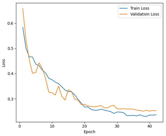
Figure 3.
Training and Validation Loss for ViTGNN Model.
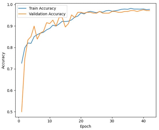
Figure 4.
Training and Validation Accuracy for ViTGNN Model.
The ROC curve in Figure 5 provides further evidence of ViTGNN’s superior classification capabilities. The model achieves an AUC score of 0.9869, indicating exceptional performance in distinguishing between classes. This high AUC score reflects the ability of ViTGNN to minimize false positives and false negatives, which is essential in high-stakes applications such as medical imaging. The superior performance of ViTGNN can be attributed to its advanced architectural design, which incorporates graph-based learning and visual transformers. This combination enables the model to leverage both spatial and contextual relationships in the data, leading to enhanced feature extraction and representation. The results indicate that ViTGNN not only excels in predictive accuracy but also maintains a consistent balance across all metrics, making it highly reliable for real-world applications.
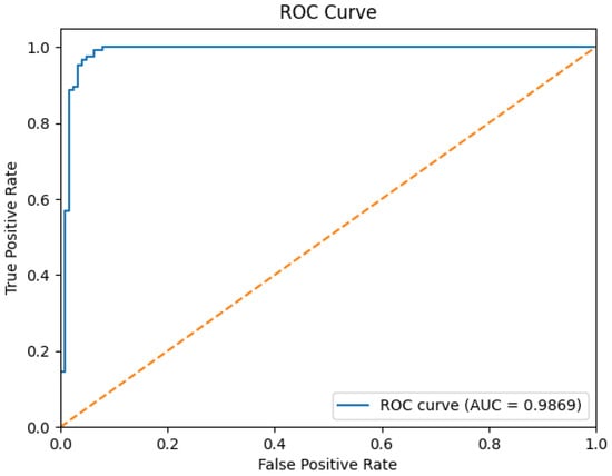
Figure 5.
ROC curve for the ViTGNN model. Note: The yellow dotted diagonal line in the ROC curve represents the performance of a random classifier and serves as a baseline, where the True Positive Rate (TPR) equals the False Positive Rate (FPR). That is, any model performing above this line demonstrates predictive power better than random guessing. In this plot, the solid blue line (AUC = 0.9869) significantly exceeds the diagonal, indicating the excellent classification performance of our proposed ViTGNN model.
In general, the results highlight ViTGNN as a state-of-the-art solution that outperforms established methods and sets a new benchmark for classification tasks. Its consistent performance across metrics demonstrates its potential in critical applications, paving the way for further research and optimization in related fields.
4.3. Generalizability of the Proposed Model and Ablation Study
4.3.1. Generalizability of the Proposed Model:
In order evaluate the performance of the proposed model, we tested it on two external chest X-ray datasets that varied substantially in disease categories, imaging protocols, and patient populations (Table 3).
Table 3.
Proposed model on Tuberculosis and Pneumonia datasets.
1. Tuberculosis (TB) Chest X-ray Dataset: This dataset, Figure 6, was compiled through a collaboration between Qatar University, the University of Dhaka, and medical institutions in Bangladesh and Malaysia. It consists of 700 publicly available TB-positive chest X-ray images and approximately 3500 normal cases [49]. These images were collected from various clinical settings and provide a valuable benchmark for testing cross-condition model generalization beyond COVID-19.
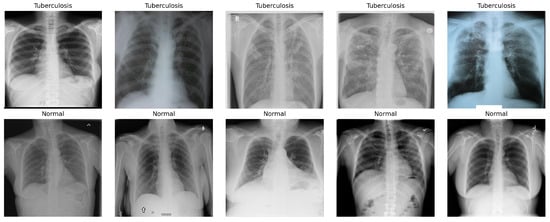
Figure 6.
Sample images of Tuberculosis (TB) Chest X-ray Dataset.
2. Pneumonia Chest X-ray Dataset: Sourced from pediatric patients aged 1 to 5 years at Guangzhou Women and Children’s Medical Center, this dataset, Figure 7, comprises 5863 anterior/posterior chest X-ray images labeled as pneumonia and normal [50].
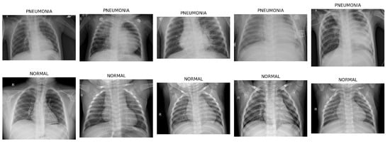
Figure 7.
Sample images of Pneumonia Chest X-ray Dataset.
4.3.2. Ablation Study
We conducted an ablation study to evaluate the contribution of each component within the proposed hybrid CNN-GNN-ViT model. The effectiveness of each stage was systematically assessed and measured by its impact on classification performance using metrics such as accuracy, precision, recall, and F1-score.
CNN Only
In this stage, we evaluated a Convolutional Neural Network (CNN) composed of convolutional and pooling layers, batch normalization, dropout regularization, and fully connected layers. This model primarily captures local spatial features within chest X-ray images. In the Tuberculosis dataset, the CNN achieved an accuracy of 91.67%, a precision of 95.45%, a recall of 75.00%, and an F1-score of 80.95%. On the Pneumonia dataset, the same model yielded 86.02% accuracy, 82.14% precision, 80.33% recall, and an F1-score of 81.16%. While the CNN was capable of detecting prominent local features associated with pulmonary diseases, its limited receptive field hindered the ability to model long-range spatial dependencies across image regions.
CNN + GNN
To address the limitations of local feature modeling, we augmented the CNN with a Graph Neural Network (GNN) in Stage 2. This hybrid CNN-GNN architecture used a grid-based graph structure to model spatial relationships among regional features. In the Tuberculosis dataset, the CNN-GNN model achieved better performance, with an accuracy of 92.14%, a precision of 95.69%, a recall of 76.43%, and an F1-score of 82.28%. For the Pneumonia dataset, the model achieved 85.25% accuracy, 80.60% precision, 81.04% recall, and 80.81% F1-score. The improvement, especially in F1-score and recall, suggests that the GNN component improves global context understanding, allowing the model to detect subtle, spatially diffuse patterns commonly seen in respiratory infections.
Our proposed ViTGNN model, a novel hybrid architecture that combines a Vision Transformer (ViT) with a Convolutional Neural Network and a Graph Neural Network, demonstrated consistently superior performance on both the Tuberculosis and Pneumonia datasets (see Table 3). This architecture effectively uses the ViT’s global self-attention mechanism along with the CNN’s local feature extraction and the GNN’s capacity to model spatial relationships among image regions. Specifically, on the Tuberculosis dataset, ViTGNN achieved an accuracy of 98.81%, a precision of 99.30%, a recall of 96.43%, and an F1-score of 97.79%. On the Pneumonia dataset, it recorded 95.59% accuracy, 92.68% precision, 97.04% recall, and a 94.52% F1-score. Remarkably, although ViTGNN was trained exclusively on datasets, it maintained high performance on both target datasets without requiring additional fine-tuning. This suggests a substantial degree of feature generalizability and robustness to domain shifts, emphasizing the model’s potential for broader clinical applicability across diverse respiratory pathologies and imaging conditions.
4.4. Computational Cost
We evaluate the trade-off between model performance and resource usage and consider the computational efficiency of all model variants across three medical imaging datasets: SARS-CoV-2, Tuberculosis, and Pneumonia. The comparison focused on two key metrics: total inference time and computational cost, both measured in seconds see Table 4.
Table 4.
Comparison of inference time and computational cost (in seconds).
Computational cost refers to the time required to complete the training of each model. This include forward and backward passes, weight updates and optimizer operations across all training epochs. It reflects the resource demands of the model in term of processor (CPU/GPU) usage, memory consumption and processing latency. Inference time, on the other hand, measures the duration required by a trained model to generate predictions on unseen test data. Specifically, it captures the average time taken for a single forward pass through the network per input sample during the testing phase [51,52].
Across all datasets, the CNN model consistently exhibited the lowest computational demands. Specifically, it completed inference in 0.72 s on the SARS-CoV-2 dataset with a computational cost of 86.09 s, followed by 2.16 s and 224.33 s for the Tuberculosis dataset and 2.88 s and 295.48 s for the Pneumonia dataset. This efficiency is attributed to its relatively lightweight and straightforward architecture, making it ideal for deployment in real-time or resource-constrained clinical environments.
In contrast, the CNN-GNN model introduced a substantial increase in both inference time and computational cost. On the SARS-CoV-2 dataset, inference required 21.43 s and incurred a computational cost of 967.29 s. Similar patterns were observed for the Tuberculosis (37.43 s, 1703.91 s) and Pneumonia (46.27 s, 2100.16 s) datasets. This increase is due to the added complexity of graph construction and the iterative message-passing operations inherent to Graph Neural Networks (GNNs).
The most computationally demanding model was the full hybrid ViTGNN, see Table 4 which integrates a Vision Transformer (ViT) with both CNN and GNN components. For the SARS-CoV-2 dataset, ViTGNN required 22.10 s for inference and a total computational cost of 8902.39 s. For the Tuberculosis and Pneumonia datasets, the respective values rose to 38.16 s and 11,009.81 s, and 47.60 s and 11,836.54 s. This overhead is attributed to the self-attention mechanisms and the model’s deeper and more parameter-intensive architecture.
Overall, while ViTGNN incurs the highest computational burden, its superior diagnostic accuracy and robust generalization performance may justify its use in scenarios where processing time is less critical than predictive precision.
5. Conclusions
This research highlights the effectiveness of the ViTGNN framework in addressing the challenge of SARS-CoV-2 detection from CT scan images. Combining the strengths of Convolutional Neural Networks and Graph Neural Networks (GNNs) for detailed feature extraction and Vision Transformers (ViTs) for high-level feature classification, ViTGNN has demonstrated superior diagnostic accuracy. Through a comprehensive experimental setup, the framework consistently achieved exceptional performance metrics, including high accuracy, precision, recall, F1-score, and AUC, validating its utility in medical imaging applications. The use of advanced preprocessing techniques ensured that the input data was optimized for feature extraction, further enhancing the model’s diagnostic capabilities. In addition, the efficient use of computational resources, coupled with techniques such as early stopping, demonstrated the model’s ability to balance performance and computational efficiency effectively. The results confirm the potential of ViTGNN for SARS-CoV-2 detection and highlight its applicability to larger healthcare challenges that involve complex imaging data. Its ability to generalize across various scenarios and provide consistent performance makes it a promising tool for integration into clinical workflows.
6. Limitation
The proposed ViTGNN model demonstrates strong performance in COVID-19 detection from CT scan images; however, several limitations must be acknowledged. Due to the high computational cost and resource constraints associated with training the model, only a single evaluation run was performed. Although this run produced favorable performance metrics, the absence of repeated trials limits the ability to report variability measures such as standard deviations or to perform statistical significance tests. In addition, the current model lacks integrated explainability mechanisms, and the computational complexity introduced by the Vision Transformer component results in increased training and inference time.
Future Work
Future work will address the limitations mentioned earlier and further advance the ViTGNN to enhance its clinical viability and trustworthiness. We will conduct multiple experimental runs using different random seeds to enable statistical effectiveness through the computation of confidence intervals and the application of hypothesis testing methods such as paired t-tests. This will strengthen the reproducibility and generalizability of performance outcomes. In parallel, we will focus on improving the model’s interpretability and transparency by integrating explainable AI (XAI) methods. In addition to graph-based and gradient-based approaches such as GNNExplainer, Layer-wise Relevance Propagation (LRP), and Grad-CAM, we plan to explore recent developments in Vision Transformer explainability. Specifically, we will investigate ICEv2 for patch-wise, class-discriminative visualization without modifying the core architecture (Choi et al. [19]), Transformer Input Sampling (TIS) for perturbation-free token-based saliency mapping (Englebert et al. [21]), and TRAM for efficient token pruning through attention-based centrality (Marchetti et al. [20]).
Moreover, wavelet-based super-resolution methods have demonstrated promise in enhancing fine-grained features crucial for accurate medical diagnosis. Yu et al. [14] introduced a WPRNN constrained by wavelet energy entropy, which fuses shallow and deep features across resolutions to improve perceptual quality and preserve subtle anatomical details. Although our current ViTGNN framework emphasizes end-to-end classification, integrating such low-level vision enhancements in future extensions could further improve feature extraction and classification performance.
Author Contributions
Conceptualization, K.A., A.W., T.A. and L.A.; Data curation, K.A.; Investigation, K.A., A.W., T.A. and L.A.; Methodology, K.A., Q.W. and J.F.; Project administration, K.A.; Resources, K.A., Q.W. and J.F.; Implementation, K.A.; Supervision, Q.W. and J.F.; Validation, K.A., Q.W. and J.F.; Visualization, K.A.; Writing—original draft preparation, K.A., A.W., T.A. and L.A.; Writing—review and editing, K.A., Q.W. and J.F. All authors have read and agreed to the published version of the manuscript.
Funding
This work was supported by the U.S. National Science Foundation (NSF) under Grant No. 2447364. Any opinions, findings, and conclusions or recommendations expressed in this material are those of the authors and do not necessarily reflect the views of the National Science Foundation.
Data Availability Statement
The datasets used in this study are publicly available at the following sources: SARS-CoV-2 CT Scan Dataset (https://www.kaggle.com/datasets/plameneduardo/sarscov2-ctscan-dataset, accessed on 10 December 2024); Chest X-ray Pneumonia Dataset (https://www.kaggle.com/datasets/paultimothymooney/chest-xray-pneumonia, accessed on 6 June 2025); and Tuberculosis Chest X-ray Dataset (https://www.kaggle.com/datasets/tawsifurrahman/tuberculosis-tb-chest-xray-dataset, accessed on 6 June 2025).
Acknowledgments
The authors acknowledge the Department of Computer and Information Sciences, Towson University, Maryland, USA, for providing the computational resources and academic environment that supported this study. Access to high-level computing resources such as the NVIDIA GeForce RTX 3090 GPU significantly facilitated experimental design, data analysis, and overall research quality. All content was thoroughly reviewed and revised by the authors, who take full responsibility for the final version of this publication.
Conflicts of Interest
The authors declare no conflicts of interest.
Abbreviations
The following abbreviations are used in this manuscript:
| ReLU | Rectified Linear Unit |
| GCN | Graph Convolutional Network |
| CNN | Convolutional Neural Network |
| GNN | Graph Neural Network |
| ViT | Vision Transformer |
| ROC | Receiver Operating Characteristic |
| SARS-CoV-2 | Severe Acute Respiratory Syndrome Coronavirus 2 |
| AUC | Area Under Curve |
| CLAHE | Contrast-Limited Adaptive Histogram Equalization |
| CT | Computed Tomography |
| VITGNN | Vision Transformer, Graph Neural Network, and Convolutional Neural Network |
References
- Jaiswal, A.; Gianchandani, N.; Singh, D.; Kumar, V.; Kaur, M. Classification of the COVID-19 infected patients using DenseNet201 based deep transfer learning. J. Biomol. Struct. Dyn. 2021, 39, 5682–5689. [Google Scholar] [CrossRef] [PubMed]
- Afshar, P.; Heidarian, S.; Enshaei, N.; Naderkhani, F.; Rafiee, M.J.; Oikonomou, A.; Fard, F.B.; Samimi, K.; Plataniotis, K.N.; Mohammadi, A. COVID-CT-MD, COVID-19 computed tomography scan dataset applicable in machine learning and deep learning. Sci. Data 2021, 8, 121. [Google Scholar] [CrossRef] [PubMed]
- Sahoo, P.; Saha, S.; Mondal, S.; Chowdhury, S.; Gowda, S. Vision Transformer-Based Federated Learning for COVID-19 Detection Using Chest X-Ray. In Proceedings of the 29th International Conference on Neural Information Processing, Virtual Event, 22–26 November 2022; Part VII. Springer: Cham, Switzerland, 2023; Volume 1794, pp. 77–88. [Google Scholar] [CrossRef]
- Wang, Z.; Liu, Q.; Dou, Q. Contrastive cross-site learning with redesigned net for COVID-19 CT classification. IEEE J. Biomed. Health Inform. 2020, 24, 2806–2813. [Google Scholar] [CrossRef]
- Soares, E.; Angelov, P.; Biaso, S.; Cury, M.; Abe, D. A large multiclass dataset of CT scans for COVID-19 identification. Evol. Syst. 2024, 15, 635–640. [Google Scholar] [CrossRef]
- Ibrahim, M.R.; Youssef, S.M.; Fathalla, K.M. Abnormality detection and intelligent severity assessment of human chest computed tomography scans using deep learning: A case study on SARS-COV-2 assessment. J. Ambient. Intell. Humaniz. Comput. 2023, 14, 5665–5688. [Google Scholar] [CrossRef]
- Parikh, D.; Fein-Ashley, J.; Ye, T.; Kannan, R.; Prasanna, V. ClusterViG: Efficient Globally Aware Vision GNNs via Image Partitioning. arXiv 2025, arXiv:2501.10640. [Google Scholar]
- Sahoo, P.; Saha, S.; Mondal, S.; Gowda, S. Vision transformer based COVID-19 detection using chest ct-scan images. In Proceedings of the 2022 IEEE-EMBS International Conference on Biomedical and Health Informatics (BHI), Ioannina, Greece, 27–30 September 2022; pp. 1–4. [Google Scholar]
- Than, J.C.; Thon, P.L.; Rijal, O.M.; Kassim, R.M.; Yunus, A.; Noor, N.M.; Then, P. Preliminary study on patch sizes in vision transformers (vit) for COVID-19 and diseased lungs classification. In Proceedings of the 2021 IEEE National Biomedical Engineering Conference (NBEC), Kuala Lumpur, Malaysia, 9–10 November 2021; pp. 146–150. [Google Scholar]
- Xu, H.; Wu, Y. G2ViT: Graph neural network-guided vision transformer enhanced network for retinal vessel and coronary angiograph segmentation. Neural Netw. 2024, 176, 106356. [Google Scholar] [CrossRef]
- Mondal, A.K.; Bhattacharjee, A.; Singla, P.; Prathosh, A. xViTCOS: Explainable vision transformer based COVID-19 screening using radiography. IEEE J. Transl. Eng. Health Med. 2021, 10, 1–10. [Google Scholar] [CrossRef]
- Wang, Y.; Deng, Y.; Zheng, Y.; Chattopadhyay, P.; Wang, L. Vision Transformers for Image Classification: A Comparative Survey. Technologies 2025, 13, 32. [Google Scholar] [CrossRef]
- Dosovitskiy, A.; Beyer, L.; Kolesnikov, A.; Weissenborn, D.; Zhai, X.; Unterthiner, T.; Dehghani, M.; Minderer, M.; Heigold, G.; Gelly, S.; et al. An image is worth 16x16 words: Transformers for image recognition at scale. arXiv 2020, arXiv:2010.11929. [Google Scholar]
- Yu, Y.; She, K.; Shi, K.; Cai, X.; Kwon, O.M.; Soh, Y. Analysis of medical images super-resolution via a wavelet pyramid recursive neural network constrained by wavelet energy entropy. Neural Netw. 2024, 178, 106460. [Google Scholar] [CrossRef]
- Zhang, L.; Wen, Y. A transformer-based framework for automatic COVID19 diagnosis in chest CTs. In Proceedings of the IEEE/CVF International Conference on Computer Vision, Montreal, BC, Canada, 11–17 October 2021; pp. 513–518. [Google Scholar]
- Zhang, P.; Yan, Y.; Zhang, X.; Li, C.; Wang, S.; Huang, F.; Kim, S. TransGNN: Harnessing the collaborative power of transformers and graph neural networks for recommender systems. In Proceedings of the 47th International ACM SIGIR Conference on Research and Development in Information Retrieval, (SIGIR ’24), Washington, DC, USA, 14–18 July 2024; pp. 1285–1295. [Google Scholar]
- Shome, D.; Kar, T.; Mohanty, S.N.; Tiwari, P.; Muhammad, K.; AlTameem, A.; Zhang, Y.; Saudagar, A.K.J. Covid-transformer: Interpretable covid-19 detection using vision transformer for healthcare. Int. J. Environ. Res. Public Health 2021, 18, 11086. [Google Scholar] [CrossRef]
- Xiao, X.; Kong, Y.; Li, R.; Wang, Z.; Lu, H. Transformer with convolution and graph-node co-embedding: An accurate and interpretable vision backbone for predicting gene expressions from local histopathological image. Med. Image Anal. 2024, 91, 103040. [Google Scholar] [CrossRef]
- Choi, H.; Jin, S.; Han, K. ICEv2: Interpretability, Comprehensiveness, and Explainability in Vision Transformer. Int. J. Comput. Vis. 2025, 133, 2487–2504. [Google Scholar] [CrossRef]
- Marchetti, M.; Traini, D.; Ursino, D.; Virgili, L. Efficient token pruning in Vision Transformers using an attention-based Multilayer Network. Expert Syst. Appl. 2025, 279, 127449. [Google Scholar] [CrossRef]
- Englebert, A.; Stassin, S.; Nanfack, G.; Mahmoudi, S.A.; Siebert, X.; Cornu, O.; De Vleeschouwer, C. Explaining through Transformer Input Sampling. In Proceedings of the IEEE/CVF International Conference on Computer Vision Workshops (ICCVW), Paris, France, 2–6 October 2023; pp. 806–815. [Google Scholar] [CrossRef]
- Soares, E.; Angelov, P.; Biaso, S.; Froes, M.H.; Abe, D.K. SARS-CoV-2 CT-scan dataset: A large dataset of real patients CT scans for SARS-CoV-2 identification. MedRxiv 2020. [Google Scholar] [CrossRef]
- Chetoui, M.; Akhloufi, M.A. Explainable Vision Transformers and Radiomics for COVID-19 Detection in Chest X-rays. J. Clin. Med. 2022, 11, 3013. [Google Scholar] [CrossRef]
- Nguyen, V.B.; Hy, T.S.; Tran-Thanh, L.; Nghiem, N. Predicting COVID-19 pandemic by spatio-temporal graph neural networks: A New Zealand’s study. arXiv 2023, arXiv:2305.07731. [Google Scholar]
- Chen, J.; Wu, L.; Zhang, J.; Zhang, L.; Gong, D.; Zhao, Y.; Chen, Q.; Huang, S.; Yang, M.; Yang, X.; et al. Deep learning-based model for detecting 2019 novel coronavirus pneumonia on high-resolution computed tomography. Sci. Rep. 2020, 10, 19196. [Google Scholar] [CrossRef]
- Wang, L.; Lin, Z.Q.; Wong, A. COVID-Net: A tailored deep convolutional neural network design for detection of COVID-19 cases from chest X-ray images. Sci. Rep. 2020, 10, 1–12. [Google Scholar] [CrossRef]
- Hu, S.; Gao, Y.; Niu, Z.; Jiang, Y.; Li, L.; Xiao, X.; Wang, M.; Fang, E.F.; Menpes-Smith, W.; Xia, J.; et al. Weakly supervised deep learning for COVID-19 infection detection and classification from CT images. IEEE Access 2020, 8, 118869–118883. [Google Scholar] [CrossRef]
- Wang, J.; Bao, Y.; Wen, Y.; Lu, H.; Luo, H.; Xiang, Y.; Li, X.; Liu, C.; Qian, D. Prior-attention residual learning for more discriminative COVID-19 screening in CT images. IEEE Trans. Med. Imaging 2020, 39, 2572–2583. [Google Scholar] [CrossRef] [PubMed]
- Shibly, K.; Dey, R.; Rahman, M.T.; Shah, F.; Rahman, T.; Sarker, M.H.; Islam, M.N.; Saba, T.; Arshad, H.; Rahman, M.M. COVID Faster R-CNN: A Novel Deep Learning Framework for COVID-19 Detection from Chest X-Ray Images. Comput. Biol. Med. 2021, 132, 104306. [Google Scholar] [CrossRef]
- Song, Y.; Zheng, S.; Li, L.; Zhang, X.; Zhang, X.; Huang, Z.; Chen, J.; Wang, R.; Zhao, H.; Chong, Y.; et al. Deep learning enables accurate diagnosis of novel coronavirus (COVID-19) with CT images. IEEE Trans. Med. Imaging 2020, 39, 2625–2635. [Google Scholar] [CrossRef] [PubMed]
- Loey, M.; Smarandache, F.; Khalifa, N. Within the Lack of Chest COVID-19 X-ray Dataset: A Novel Detection Model Based on GAN and Deep Transfer Learning. Symmetry 2020, 12, 651. [Google Scholar] [CrossRef]
- Salehi, S.; Abedi, A.; Balakrishnan, S.; Gholamrezanezhad, A. Coronavirus Disease 2019 (COVID-19): A Systematic Review of Imaging Findings in 919 Patients. AJR Am. J. Roentgenol. 2020, 215, 87–93. [Google Scholar] [CrossRef]
- Li, L.; Qin, L.; Xu, Z.; Lu, H.; Luo, H.; Xiang, Y.; Li, X.; Liu, C.; Qian, D. Using artificial intelligence to detect COVID-19 and community-acquired pneumonia based on pulmonary CT: Evaluation of the diagnostic accuracy. Radiology 2020, 296, E65–E71. [Google Scholar] [CrossRef]
- Wang, X.; Deng, X.; Fu, Q.; Zhou, Q.; Feng, J.; Ma, H.; Liu, W.; Zheng, C. A weakly-supervised framework for COVID-19 classification and lesion localization from chest CT. IEEE Trans. Med. Imaging 2020, 39, 2615–2625. [Google Scholar] [CrossRef]
- Ozturk, T.; Talo, M.; Yildirim, E.A.; Baloglu, U.B.; Yildirim, O.; Acharya, U.R. Automated detection of COVID-19 cases using deep neural networks with X-ray images. Comput. Biol. Med. 2020, 121, 103792. [Google Scholar] [CrossRef]
- Heidari, M.; Mirniaharikandehei, S.; Khuzani, A.Z.; Danala, G.; Qiu, Y.; Zheng, B. Improving the performance of CNN to predict the likelihood of COVID-19 using chest X-ray images with preprocessing algorithms. Int. J. Med. Inform. 2020, 144, 104284. [Google Scholar] [CrossRef]
- Ouchicha, C.; Ammor, O.; Meknassi, M. CVDNet: A novel deep learning architecture for detection of coronavirus (COVID-19) from chest X-ray images. Chaos Solitons Fractals 2020, 140, 110245. [Google Scholar] [CrossRef] [PubMed]
- Chowdhury, M.E.; Rahman, T.; Khandakar, A.; Mazhar, R.; Kadir, M.A.; Mahbub, Z.; Islam, M.T.; Ayari, M.A.; Al-Emadi, N.; Reaz, M.B.I. Can AI Help in Screening Viral and COVID-19 Pneumonia? IEEE Access 2020, 8, 132665–132676. [Google Scholar] [CrossRef]
- Zheng, C.; Deng, X.; Fu, Q.; Zhou, Q.; Feng, J.; Ma, H.; Liu, W.; Wang, X. Deep learning-based detection for COVID-19 from chest CT using weak label. medRxiv 2020. [Google Scholar] [CrossRef]
- Aslani, S.; Lilaonitkul, W.; Gnanananthan, V.; Raj, D.; Rangelov, B.; Young, A.L.; Hu, Y.; Taylor, P.; Alexander, D.C.; Jacob, J. Optimising Chest X-Rays for Image Analysis by Identifying and Removing Confounding Factors. arXiv 2022, arXiv:2208.10320. [Google Scholar]
- Fu, Q.; Celenk, M.; Wu, A. An improved algorithm based on CLAHE for ultrasonic well logging image enhancement. Clust. Comput. 2019, 22, 12609–12618. [Google Scholar] [CrossRef]
- Hayati, M.; Muchtar, K.; Roslidar; Maulina, N.; Syamsuddin, I.; Elwirehardja, G.N.; Pardamean, B. Impact of CLAHE-based image enhancement for diabetic retinopathy classification through deep learning. Procedia Comput. Sci. 2023, 216, 57–66. [Google Scholar] [CrossRef]
- Flusser, J.; Farokhi, S.; Höschl, C.; Suk, T.; Zitova, B.; Pedone, M. Recognition of images degraded by Gaussian blur. IEEE Trans. Image Process. 2015, 25, 790–806. [Google Scholar] [CrossRef]
- Khalifa, N.E.; Loey, M.; Mirjalili, S. A comprehensive survey of recent trends in deep learning for digital images augmentation. Artif. Intell. Rev. 2022, 55, 2351–2377. [Google Scholar] [CrossRef]
- Kim, J.W.; Khan, A.U.; Banerjee, I. Systematic review of hybrid vision transformer architectures for radiological image analysis. J. Imaging Inform. Med. 2025. [Google Scholar] [CrossRef]
- Liu, Z.Q.; Tang, P.; Zhang, W.; Zhang, Z. CNN-enhanced heterogeneous graph convolutional network: Inferring land use from land cover with a case study of park segmentation. Remote Sens. 2022, 14, 5027. [Google Scholar] [CrossRef]
- Han, K.; Wang, Y.; Guo, J.; Tang, Y.; Wu, E. Vision gnn: An image is worth graph of nodes. Adv. Neural Inf. Process. Syst. 2022, 35, 8291–8303. [Google Scholar]
- Chen, T.; Philippi, I.; Phan, Q.B.; Nguyen, L.; Bui, N.T.; Nguyen, T.T. A vision transformer machine learning model for COVID-19 diagnosis using chest X-ray images. Healthc. Anal. 2024, 5, 100332. [Google Scholar] [CrossRef]
- Rahman, T.; Khandakar, A.; Kadir, M.A.; Islam, K.R.; Islam, K.F.; Mazhar, R.; Hamid, T.; Islam, M.T.; Kashem, S.; Mahbub, Z.B.; et al. Reliable Tuberculosis Detection Using Chest X-Ray With Deep Learning, Segmentation and Visualization. IEEE Access 2020, 8, 191586–191601. [Google Scholar] [CrossRef]
- Kermany, D.S.; Goldbaum, M.; Cai, W.; Valentim, C.C.; Liang, H.; Baxter, S.L.; McKeown, A.; Yang, G.; Wu, X.; Yan, F.; et al. Identifying medical diagnoses and treatable diseases by image-based deep learning. Cell 2018, 172, 1122–1131. [Google Scholar] [CrossRef]
- Justus, D.; Brennan, J.; Bonner, S.; McGough, A.S. Predicting the Computational Cost of Deep Learning Models. In Proceedings of the 2018 IEEE International Conference on Big Data (Big Data), Seattle, WA, USA, 10–13 December 2018; pp. 3873–3882. [Google Scholar] [CrossRef]
- Zhang, H.; Huang, Y.; Wen, Y.; Yin, J.; Guan, K. InferBench: Understanding Deep Learning Inference Serving with an Automatic Benchmarking System. arXiv 2020, arXiv:2011.02327. Available online: https://arxiv.org/abs/2011.02327 (accessed on 27 June 2025).
Disclaimer/Publisher’s Note: The statements, opinions and data contained in all publications are solely those of the individual author(s) and contributor(s) and not of MDPI and/or the editor(s). MDPI and/or the editor(s) disclaim responsibility for any injury to people or property resulting from any ideas, methods, instructions or products referred to in the content. |
© 2025 by the authors. Licensee MDPI, Basel, Switzerland. This article is an open access article distributed under the terms and conditions of the Creative Commons Attribution (CC BY) license (https://creativecommons.org/licenses/by/4.0/).