
Predicting the Magnitude of Earthquakes Using Grammatical Evolution


Abstract
1. Introduction
2. Materials and Methods
2.1. The Dataset Employed
- On the Earthquake Interactive Browser platform, the “maximum earthquakes” parameter was set to 25,000 in order to extract the maximum available number of records.
- The “time range” was then adjusted to correspond to the specific year or range of years targeted for data collection.
- Subsequently, the “magnitude range” was specified, the filter was applied, and the dataset was downloaded in Excel format.
- The final dataset was further processed by creating a separate column for each variable, including the following: Year, Month, Day, Time, Latitude, Longitude, Depth, Magnitude, Magnitude Code, Region, Region Code, Lithospheric/Tectonic Plate, Lithospheric/Tectonic Plate Code, Stratovolcano, Volcanic Field, Lava Dome, Caldera, Complex, Compound, Shield, Pyroclastic, Minor, and Submarine.
2.2. Grammatical Evolution Preliminaries
- The set N represents non-terminal symbols.
- The set T contains the terminal symbols of the language.
- The symbol denotes the start symbol of the grammar.
- The set P holds the production rules of the grammar.
- Read the next element V from the current chromosome.
- Select the production rule using the following equation: Rule = V mod . The constant stands for the total number of production rules for the non-terminal symbol that is currently under processing.
2.3. The Rule Production Method
- Step 1—Initialization step.
- Set as the number of chromosomes, and as the maximum number of allowed generations.
- Set as the selection rate of the genetic algorithm, and as the corresponding mutation rate.
- Initialize the chromosomes . Each chromosome is considered a set of randomly selected positive integers.
- Set , the generation counter.
- Step 2—Fitness calculation step.
- For perform the following:
- (a)
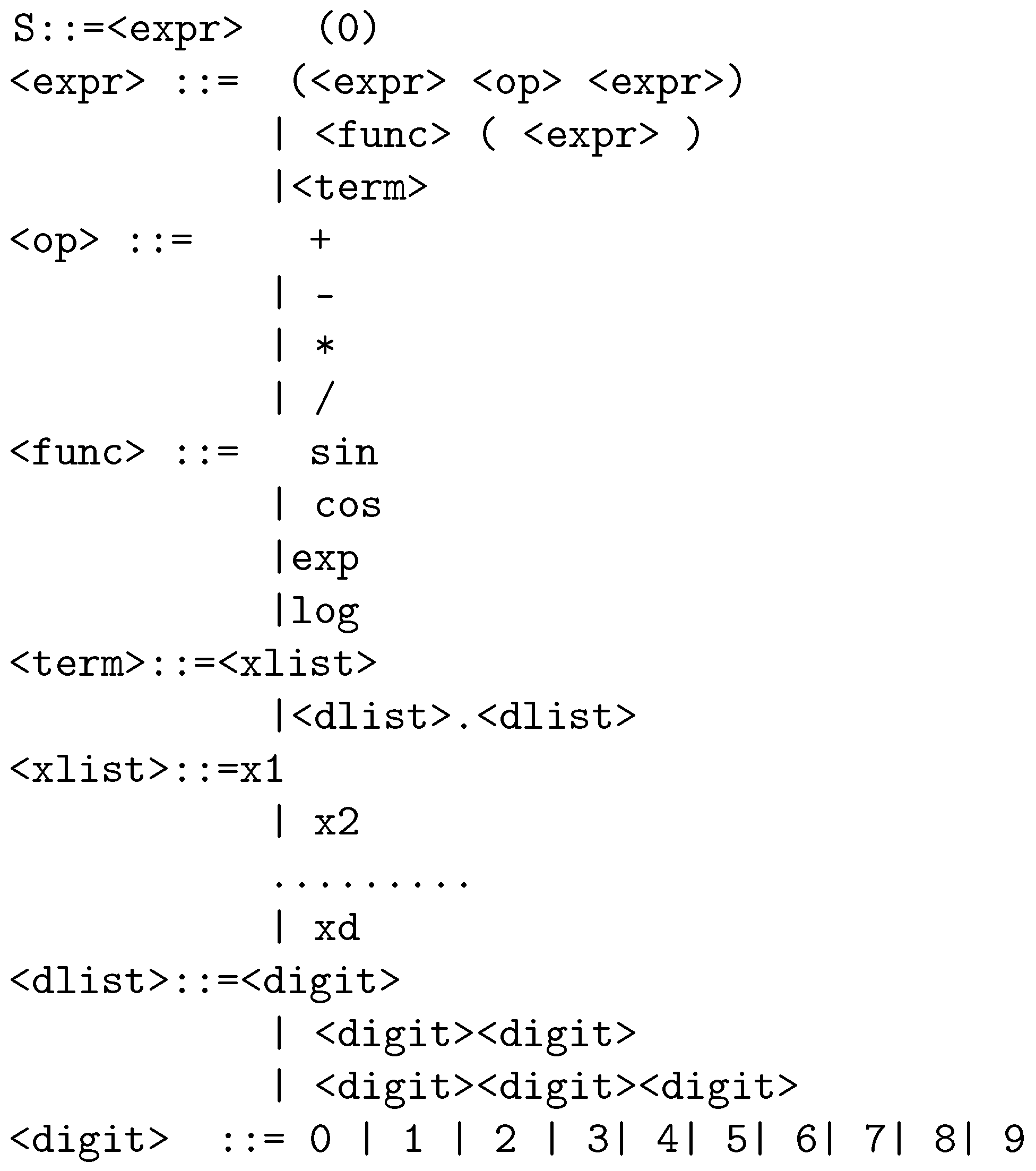
- Create the program for the chromosome using the grammar of Figure 3 and the Grammatical Evolution production mechanism.
- (b)
- Set as the fitness value for chromosome the training error of the produced program, calculated as follows:The set defines the training set of the objective problem, where the value is considered as the actual output for the input pattern . In the current implementation of Grammatical Evolution, the fitness function is defined as the sum of squared errors between the predicted and actual earthquake magnitudes across the training set. This fitness function is crucial in guiding the evolutionary process by favoring candidate solutions (programs) that minimize prediction error. As earthquake magnitude prediction is a regression task, this formulation ensures that evolved models are optimized for minimizing the deviation from actual magnitudes.
- End For
- Step 3—Genetic operations step.
- Select the best chromosomes from the current population. These chromosomes will be transferred intact to the next generation.
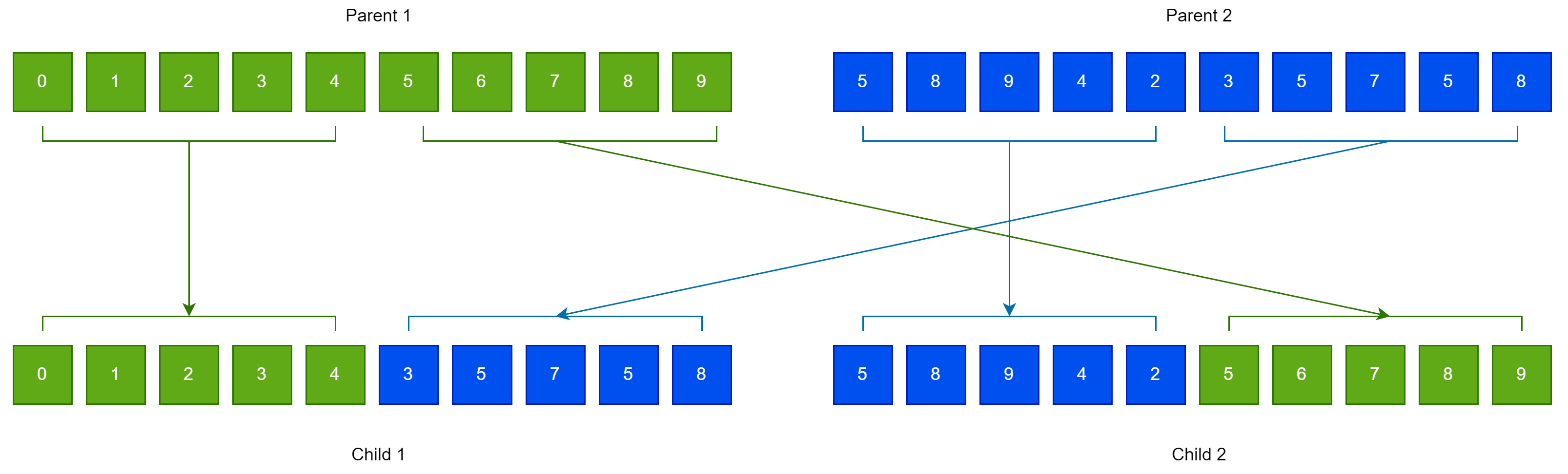
- Create chromosomes with the assistance of the one-point crossover shown graphically in Figure 4. For every couple of created offsprings, two chromosomes should be chosen from the current population using tournament selection.
- Mutation procedure: For every element of each chromosome, a random number is selected. The corresponding element is altered randomly when .
- Step 4—Termination check step.
- Set .
- If , go to the fitness calculation step.
2.4. Constructed Neural Networks
- Step 1—Initialization step.
- Define as the number of chromosomes in the genetic population and as the total number of allowed generations.
- Set as the used selection rate and as the used mutation rate.
- Initialize the chromosomes . Each chromosome is considered as a set of randomly selected positive integers.
- Set as the generation counter.
- Step 2—Fitness calculation step.
- For , perform the following:
- (a)
- Obtain the chromosome .
- (b)
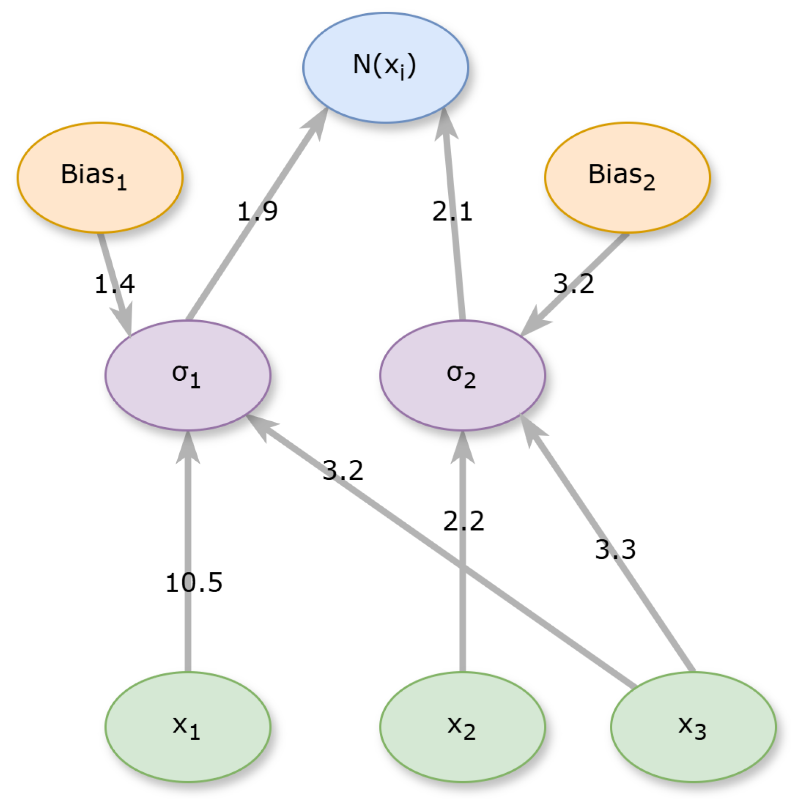
- Create the corresponding neural network for this chromosome using the grammar in Figure 5.
- (c)
- Calculate the associated fitness value as the training error of network , defined as follows:
- End For
- Step 3—Application of genetic operations. Apply the same genetic operations as in the algorithm of Section 2.3.
- Step 4—Termination check step.
- Set .
- Terminate if .
- Go to the fitness calculation step.
2.5. The Feature Construction Method
- Initialization step.
- (a)
- Set the parameters of the method: —the number of chromosomes, —the maximum number of allowed generations, —the selection rate, and —the mutation rate.
- (b)
- Initialize the chromosomes as sets of random integers.
- (c)
- Set as the number of constructed features.
- (d)
- Set , the generation counter.
- Fitness calculation step.
- (a)
- For perform the following:
- Produce artificial features for the processed chromosome using the grammar in Figure 7.
- Modify the original training set using the constructed features .
- Apply a machine learning model, denoted as , to the modified set and define as the fitness value the training error of .
- (b)
- End For
- Genetic operations step. Apply the same genetic operations as applied in the algorithm in Section 2.3.
- Termination check step.
- (a)
- Set.
- (b)
- Terminate when .
- (c)
- Go to the fitness calculation step.
3. Experimental Results
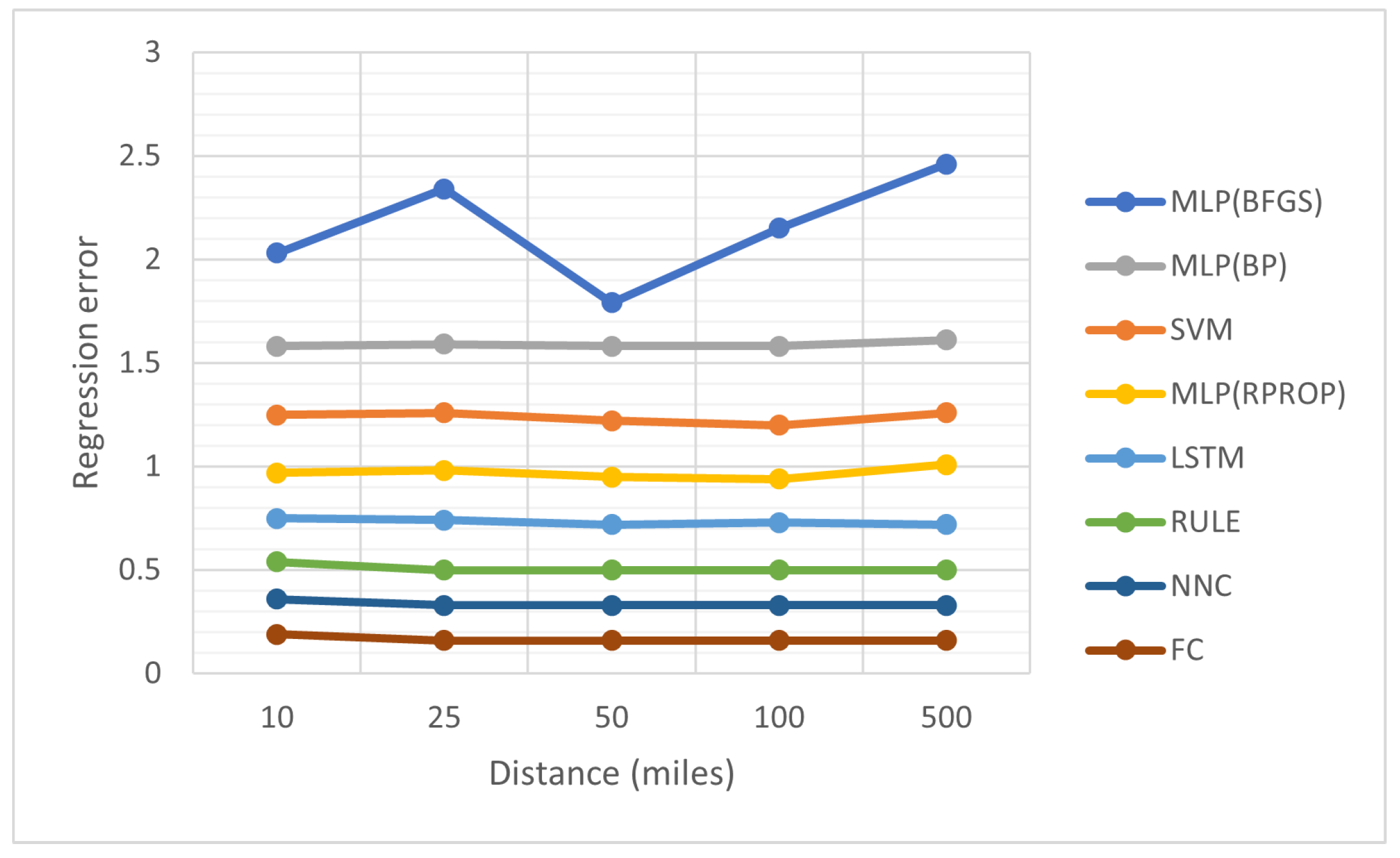
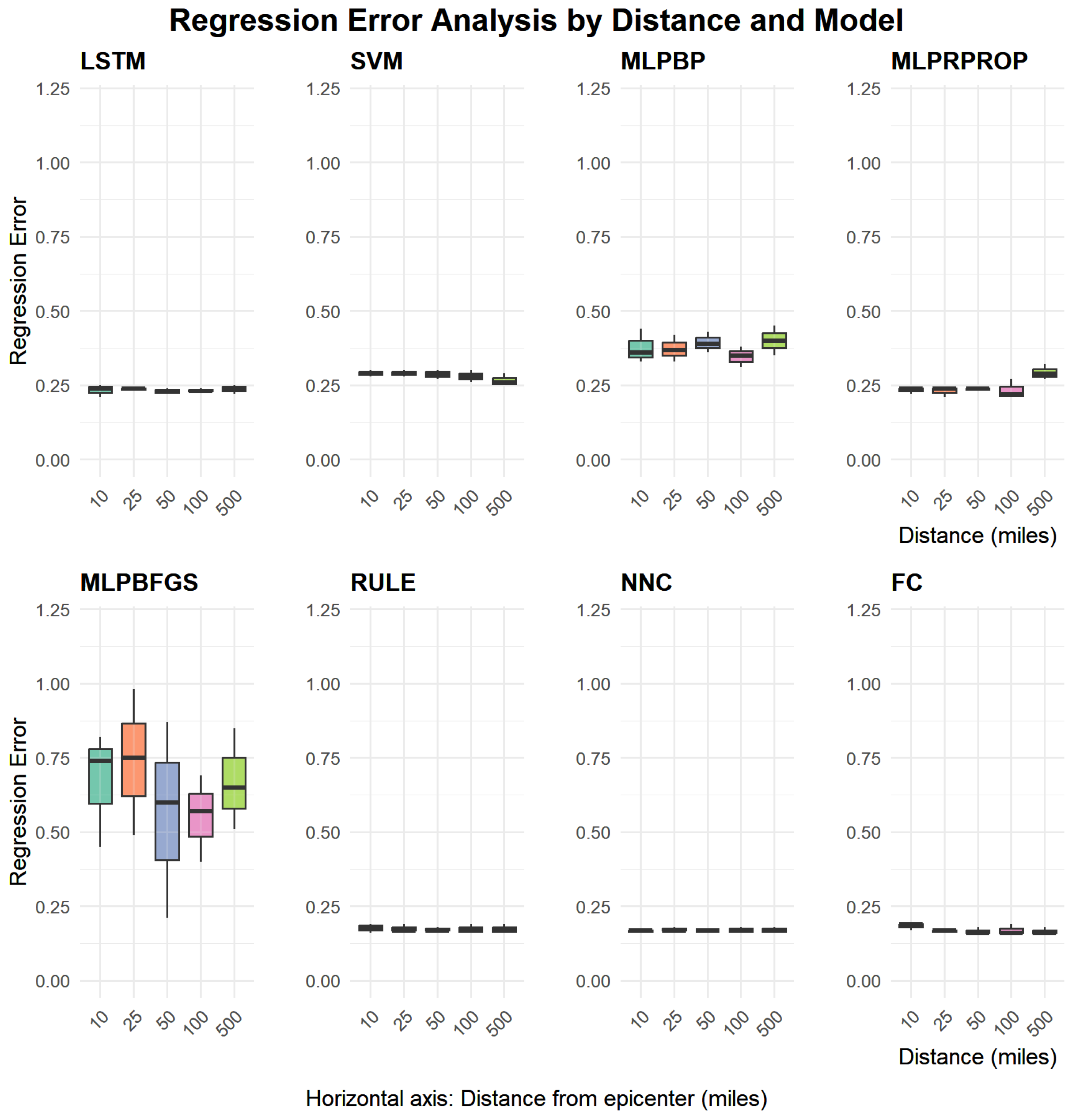
- The column YEAR denotes the recording year for the earthquakes.
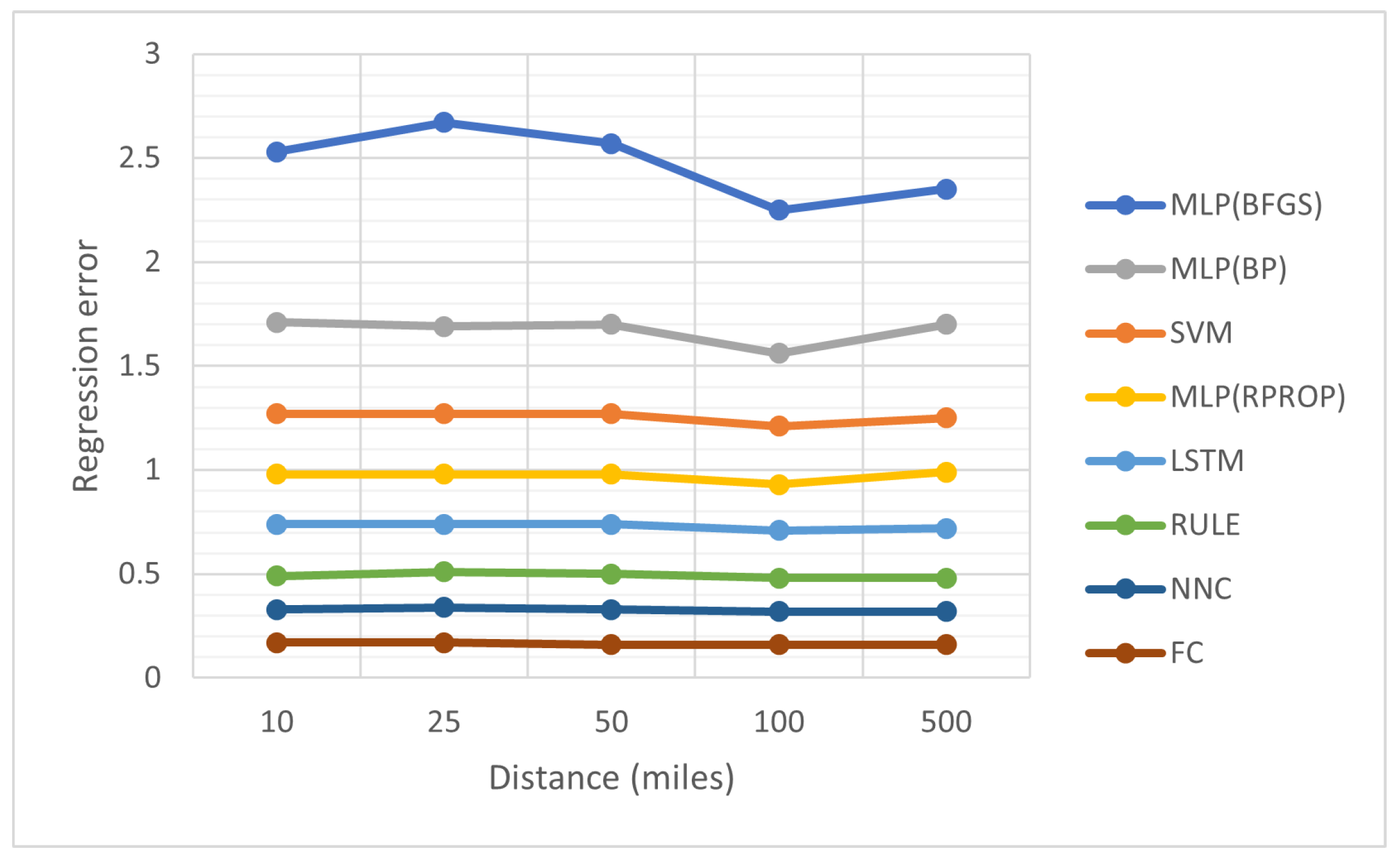
- The column denotes the critical distance, expressed in miles, used in the preprocessing of the earthquake data.
- The column MLP(BP) denotes the incorporation of the Back Propagation algorithm [65] in the training of a neural network with processing nodes.
- The column MLP(BFGS) denotes the usage of the BFGS optimization procedure [68] for the training of an artificial neural network with processing nodes.
- The column RULE denotes the incorporation of the rule construction method, described in Section 2.3.
- The column NNC represents the usage of the Neural Network Construction method, provided in Section 2.4.
- The column FC represents the usage of the Feature Construction technique, outlined in Section 2.5.
- The row AVERAGE represents the average error for all years and critical distances.
4. Conclusions
Author Contributions
Funding
Institutional Review Board Statement
Informed Consent Statement
Data Availability Statement
Conflicts of Interest
References
- Seismograph. Britannica, Earth Sciences. Available online: https://www.britannica.com/science/seismograph (accessed on 20 May 2025).
- Robert Mallet. Britannica, Civil Engineering. Available online: https://www.britannica.com/biography/Robert-Mallet (accessed on 20 May 2025).
- Can You Predict Earthquakes? United States Geological Survey. Available online: https://www.usgs.gov/faqs/can-you-predict-earthquakes (accessed on 20 May 2025).
- Bergen, K.J.; Chen, T.; Li, Z. Preface to the focus section on machine learning in seismology. Seismol. Res. Lett. 2019, 90, 477–480. [Google Scholar] [CrossRef]
- Hutchison, A. How machine learning might unlock earthquake prediction. MIT Technology Review. 29 December 2023. Available online: https://www.technologyreview.com/2023/12/29/1084699/machine-learning-earthquake-prediction-ai-artificial-intelligence/ (accessed on 20 May 2025).
- Hincks, T.; Aspinall, W.; Cooke, R.; Gernon, T. Oklahoma’s induced seismicity strongly linked to wastewater injection depth. Science 2018, 359, 1251–1255. [Google Scholar] [CrossRef]
- Obara, K. Nonvolcanic deep tremor associated with subduction in southwest Japan. Science 2002, 296, 1679–1681. [Google Scholar] [CrossRef] [PubMed]
- Obara, K.; Kato, A. Connecting slow earthquakes to huge earthquakes. Science 2016, 353, 253–257. [Google Scholar] [CrossRef] [PubMed]
- Bletery, Q.; Nocquet, J.M. The precursory phase of large earthquakes. Science 2023, 381, 297–301. [Google Scholar] [CrossRef]
- Avolio, C.; Muller, U.; Wikelski, M. The secret knowledge of animals. Max Planck Institute of Animal Behavior. 12 April 2024. Available online: https://www.ab.mpg.de/578863/news_publication_21821500_transferred?c=413930 (accessed on 20 May 2025).
- Mousavi, S.M.; Beroza, G.C. A machine-learning approach for earthquake magnitude estimation. Geophys. Res. Lett. 2020, 47, e2019GL085976. [Google Scholar] [CrossRef]
- DeVries, P.M.; Viégas, F.; Wattenberg, M.; Meade, B.J. Deep learning of aftershock patterns following large earthquakes. Nature 2018, 560, 632–634. [Google Scholar] [CrossRef]
- Ross, Z.E.; Meier, M.A.; Hauksson, E. P wave arrival picking and first-motion polarity determination with deep learning. J. Geophys. Res. Solid Earth 2018, 123, 5120–5129. [Google Scholar] [CrossRef]
- Rouet-Leduc, B.; Hulbert, C.; Lubbers, N.; Barros, K.; Humphreys, C.J.; Johnson, P.A. Machine learning predicts laboratory earthquakes. Geophys. Res. Lett. 2017, 44, 9276–9282. [Google Scholar] [CrossRef]
- Rouet-Leduc, B.; Hulbert, C.; Johnson, P.A. Continuous chatter of the Cascadia subduction zone revealed by machine learning. Nat. Geosci. 2019, 12, 75–79. [Google Scholar] [CrossRef]
- Tan, Y.J.; Waldhauser, F.; Ellsworth, W.L.; Zhang, M.; Zhu, W.; Michele, M.; Chiaraluce, L.; Beroza, G.C.; Segou, M. Machine-learning-based high-resolution earthquake catalog reveals how complex fault structures were activated during the 2016–2017 central Italy sequence. Seism. Rec. 2021, 1, 11–19. [Google Scholar] [CrossRef]
- Mousavi, S.M.; Ellsworth, W.L.; Zhu, W.; Chuang, L.Y.; Beroza, G.C. Earthquake transformer—An attentive deep-learning model for simultaneous earthquake detection and phase picking. Nat. Commun. 2020, 11, 3952. [Google Scholar] [CrossRef]
- Hsu, Y.F.; Zaliapin, I.; Ben-Zion, Y. Informative modes of seismicity in nearest-neighbor earthquake proximities. J. Geophys. Res. Solid Earth 2024, 129, e2023JB027826. [Google Scholar] [CrossRef]
- Bayliss, K.; Naylor, M.; Main, I.G. Probabilistic identification of earthquake clusters using rescaled nearest neighbour distance networks. Geophys. J. Int. 2019, 217, 487–503. [Google Scholar] [CrossRef]
- Saad, O.M.; Chen, Y.; Savvaidis, A.; Fomel, S.; Jiang, X.; Huang, D.; Oboue, Y.A.S.I.; Yong, S.; Wang, X.A.; Zhang, X.; et al. Earthquake forecasting using big data and artificial intelligence: A 30-week real-time case study in China. Bull. Seismol. Soc. Am. 2023, 113, 2461–2478. [Google Scholar] [CrossRef]
- Asim, K.M.; Martínez-Álvarez, F.; Basit, A.; Iqbal, T. Earthquake magnitude prediction in Hindukush region using machine learning techniques. Nat. Hazards 2017, 85, 471–486. [Google Scholar] [CrossRef]
- Corbi, F.; Sandri, L.; Bedford, J.; Funiciello, F.; Brizzi, S.; Rosenau, M.; Lallemand, S. Machine learning can predict the timing and size of analog earthquakes. Geophys. Res. Lett. 2019, 46, 1303–1311. [Google Scholar] [CrossRef]
- Hoque, A.; Raj, J.; Saha, A.; Bhattacharya, P. Earthquake magnitude prediction using machine learning technique. In Trends in Computational Intelligence, Security and Internet of Things: Third International Conference, ICCISIoT 2020, Tripura, India, 29–30 December 2020, Proceedings 3; Springer International Publishing: Berlin/Heidelberg, Germany, 2020; pp. 37–53. [Google Scholar]
- Zhu, C.; Cotton, F.; Kawase, H.; Nakano, K. How well can we predict earthquake site response so far? Machine learning vs physics-based modeling. Earthq. Spectra 2023, 39, 478–504. [Google Scholar] [CrossRef]
- Xiong, P.; Tong, L.; Zhang, K.; Shen, X.; Battiston, R.; Ouzounov, D.; Iuppa, R.; Crookes, D.; Long, C.; Zhou, H. Towards advancing the earthquake forecasting by machine learning of satellite data. Sci. Total Environ. 2021, 771, 145256. [Google Scholar] [CrossRef]
- Bhatia, M.; Ahanger, T.A.; Manocha, A. Artificial intelligence based real-time earthquake prediction. Eng. Appl. Artif. Intell. 2023, 120, 105856. [Google Scholar] [CrossRef]
- Earthquake Early Warning System. Japan Meteorological Agency. Available online: https://www.jma.go.jp/jma/en/Activities/eew.html (accessed on 20 May 2025).
- Earthquake Early Warning System (Japan). Wikipedia. Available online: https://en.wikipedia.org/wiki/Earthquake_Early_Warning_(Japan) (accessed on 20 May 2025).
- ShakeAlert. US Geological Survey, Earthquake Hazards Program. Available online: https://earthquake.usgs.gov/data/shakealert/ (accessed on 20 May 2025).
- ShakeAlert. Earthquake Early Warning (EEW) System. Available online: https://www.shakealert.org/ (accessed on 20 May 2025).
- Beroza, G.C.; Segou, M.; Mousavi, M.S. Machine learning and earthquake forecasting—Next steps. Nat. Commun. 2021, 12, 4761. [Google Scholar] [CrossRef]
- Mousavi, S.M.; Beroza, G.C. Machine learning in earthquake seismology. Annu. Rev. Earth Planet. Sci. 2023, 51, 105–129. [Google Scholar] [CrossRef]
- O’Neill, M.; Ryan, C. Grammatical evolution. IEEE Trans. Evol. Comput. 2001, 5, 349–358. [Google Scholar] [CrossRef]
- Backus, J.W. The Syntax and Semantics of the Proposed International Algebraic Language of the Zurich ACM-GAMM Conference. In Proceedings of the International Conference on Information Processing, UNESCO, Paris, France, 15–20 June 1959; pp. 125–132. [Google Scholar]
- Ryan, C.; Collins, J.; O’Neill, M. Grammatical evolution: Evolving programs for an arbitrary language. In Genetic Programming; EuroGP 1998; Lecture Notes in Computer Science; Banzhaf, W., Poli, R., Schoenauer, M., Fogarty, T.C., Eds.; Springer: Berlin/Heidelberg, Germany, 1998; Volume 1391. [Google Scholar]
- O’Neill, M.; Ryan, M.C. Evolving Multi-line Compilable C Programs. In Genetic Programming; EuroGP 1999; Lecture Notes in Computer Science; Poli, R., Nordin, P., Langdon, W.B., Fogarty, T.C., Eds.; Springer: Berlin/Heidelberg, Germany, 1999; Volume 1598. [Google Scholar]
- Puente, A.O.; Alfonso, R.S.; Moreno, M.A. Automatic composition of music by means of grammatical evolution. In Proceedings of the 2002 Conference on APL: Array Processing Languages: Lore, Problems, and Applications, APL ’02, Madrid, Spain, 22–25 July 2002; pp. 148–155. [Google Scholar]
- Galván-López, E.; Swafford, J.M.; O’Neill, M.; Brabazon, A. Evolving a Ms. PacMan Controller Using Grammatical Evolution. In Applications of Evolutionary Computation. EvoApplications 2010; Lecture Notes in Computer Science; Springer: Berlin/Heidelberg, Germany, 2010; Volume 6024. [Google Scholar]
- Shaker, N.; Nicolau, M.; Yannakakis, G.N.; Togelius, J.; O’Neill, M. Evolving levels for Super Mario Bros using grammatical evolution. In Proceedings of the 2012 IEEE Conference on Computational Intelligence and Games (CIG), Granada, Spain, 11–14 September 2012; pp. 304–331. [Google Scholar]
- Martínez-Rodríguez, D.; Colmenar, J.M.; Hidalgo, J.I.; Villanueva Micó, R.J.; Salcedo-Sanz, S. Particle swarm grammatical evolution for energy demand estimation. Energy Sci. Eng. 2020, 8, 1068–1079. [Google Scholar] [CrossRef]
- Ryan, C.; Kshirsagar, M.; Vaidya, G.; Cunningham, A.; Sivaraman, R. Design of a cryptographically secure pseudo random number generator with grammatical evolution. Sci. Rep. 2022, 12, 8602. [Google Scholar] [CrossRef] [PubMed]
- Martín, C.; Quintana, D.; Isasi, P. Grammatical Evolution-based ensembles for algorithmic trading. Appl. Soft Comput. 2019, 84, 105713. [Google Scholar] [CrossRef]
- Bishop, C. Neural Networks for Pattern Recognition; Oxford University Press: Oxford, UK, 1995. [Google Scholar]
- Cybenko, G. Approximation by superpositions of a sigmoidal function. Math. Control Signals Syst. 1989, 2, 303–314. [Google Scholar] [CrossRef]
- Lakkos, S.; Hadjiprocopis, A.; Compley, R.; Smith, P. A neural network scheme for earthquake prediction based on the Seismic Electric Signals. In Proceedings of the IEEE Conference on Neural Networks and Signal Processing, Ermioni, Greece, 6–8 September 1994; pp. 681–689. [Google Scholar]
- Negarestani, A.; Setayeshi, S.; Ghannadi-Maragheh, M.; Akashe, B. Layered neural networks based analysis of radon concentration and environmental parameters in earthquake prediction. J. Environ. Radioact. 2002, 62, 225–233. [Google Scholar] [CrossRef] [PubMed]
- Panakkat, A.; Adeli, H. Neural network models for earthquake magnitude prediction using multiple seismicity indicators. Int. J. Neural Syst. 2007, 17, 13–33. [Google Scholar] [CrossRef]
- Holland, J.H. Genetic algorithms. Sci. Am. 1992, 267, 66–73. [Google Scholar] [CrossRef]
- Sastry, K.; Goldberg, D.; Kendall, G. Genetic algorithms. In Search Methodologies: Introductory Tutorials in Optimization and Decision Support Techniques; Springer: Berlin/Heidelberg, Germany, 2005; pp. 97–125. [Google Scholar]
- Tsoulos, I.G. Learning Functions and Classes Using Rules. AI 2022, 3, 751–763. [Google Scholar] [CrossRef]
- Tsoulos, I.G.; Gavrilis, D.; Glavas, E. Neural network construction and training using grammatical evolution. Neurocomputing 2008, 72, 269–277. [Google Scholar] [CrossRef]
- Papamokos, G.V.; Tsoulos, I.G.; Demetropoulos, I.N.; Glavas, E. Location of amide I mode of vibration in computed data utilizing constructed neural networks. Expert Syst. Appl. 2009, 36, 12210–12213. [Google Scholar] [CrossRef]
- Christou, V.; Tsoulos, I.G.; Loupas, V.; Tzallas, A.T.; Gogos, C.; Karvelis, P.S.; Antoniadis, N.; Glavas, E.; Giannakeas, N. Performance and early drop prediction for higher education students using machine learning. Expert Syst. Appl. 2023, 225, 120079. [Google Scholar] [CrossRef]
- Toki, E.I.; Pange, J.; Tatsis, G.; Plachouras, K.; Tsoulos, I.G. Utilizing Constructed Neural Networks for Autism Screening. Appl. Sci. 2024, 14, 3053. [Google Scholar] [CrossRef]
- Gavrilis, D.; Tsoulos, I.G.; Dermatas, E. Selecting and constructing features using grammatical evolution. Pattern Recognit. Lett. 2008, 29, 1358–1365. [Google Scholar] [CrossRef]
- Park, J.; Sandberg, I.W. Universal Approximation Using Radial-Basis-Function Networks. Neural Comput. 1991, 3, 246–257. [Google Scholar] [CrossRef]
- Yu, H.; Xie, T.; Paszczynski, S.; Wilamowski, B.M. Advantages of Radial Basis Function Networks for Dynamic System Design. IEEE Trans. Ind. Electron. 2011, 58, 5438–5450. [Google Scholar] [CrossRef]
- Tsoulos, I.G.; Tzallas, A.; Tsalikakis, D. NNC: A tool based on Grammatical Evolution for data classification and differential equation solving. SoftwareX 2019, 10, 100297. [Google Scholar] [CrossRef]
- Tsoulos, I.G. QFC: A Parallel Software Tool for Feature Construction, Based on Grammatical Evolution. Algorithms 2022, 15, 295. [Google Scholar] [CrossRef]
- Hall, M.; Frank, F.; Holmes, G.; Pfahringer, B.; Reutemann, P.; Witten, I.H. The WEKA data mining software: An update. ACM Sigkdd Explor. Newsl. 2009, 11, 10–18. [Google Scholar] [CrossRef]
- Yu, Y.; Si, X.; Hu, C.; Zhang, J. A review of recurrent neural networks: LSTM cells and network architectures. Neural Comput. 2019, 31, 1235–1270. [Google Scholar] [CrossRef] [PubMed]
- Ketkar, N.; Moolayil, J.; Ketkar, N.; Moolayil, J. Introduction to pytorch. In Deep Learning with Python: Learn Best Practices of Deep Learning Models with PyTorch; Apress: New York, NY, USA, 2021; pp. 27–91. [Google Scholar]
- Xue, H.; Yang, Q.; Chen, S. SVM: Support vector machines. In The Top Ten Algorithms in Data Mining; Chapman and Hall/CRC: Boca Raton, FL, USA, 2009; pp. 51–74. [Google Scholar]
- Chang, C.C.; Lin, C.J. LIBSVM: A library for support vector machines. ACM Trans. Intell. Syst. Technol. (TIST) 2011, 2, 27. [Google Scholar] [CrossRef]
- Vora, K.; Yagnik, S. A survey on backpropagation algorithms for feedforward neural networks. Int. J. Eng. Dev. Res. 2014, 1, 193–197. [Google Scholar]
- Pajchrowski, T.; Zawirski, K.; Nowopolski, K. Neural speed controller trained online by means of modified RPROP algorithm. IEEE Trans. Ind. Inform. 2014, 11, 560–568. [Google Scholar] [CrossRef]
- Hermanto, R.P.S.; Nugroho, A. Waiting-time estimation in bank customer queues using RPROP neural networks. Procedia Comput. Sci. 2018, 135, 35–42. [Google Scholar] [CrossRef]
- Powell, M.J.D. A Tolerant Algorithm for Linearly Constrained Optimization Calculations. Math. Program. 1989, 45, 547–566. [Google Scholar] [CrossRef]


| 2010–2025 | Deaths | Injured People | Homeless People |
|---|---|---|---|
| Floods | 82,644 | 111,954 | 7,552,142 |
| Storms | 51,091 | 125,266 | 3,671,100 |
| Wildfires | 1622 | 13,810 | 94,925 |
| Earthquakes | 337,372 | 698,085 | 1,547,581 |
| 2004 | 2010 | 2012 | |
|---|---|---|---|
| Earthquakes | 126,972 | 294,432 | 370,582 |
| 0–4.9 mag | 126,003 | 292,387 | 369,101 |
| 5–5.9 mag | 893 | 1909 | 1374 |
| 6–6.9 mag | 68 | 117 | 92 |
| 7–7.9 mag | 7 | 19 | 13 |
| 8–8.9 mag | 1 | 0 | 2 |
| 9–10 mag | 1 | 0 | 0 |
| Expression | Chromosome | Operation |
|---|---|---|
| <expr> | 9,8,6,4,16,10,17,23,8,14 | |
| (<expr><op><expr>) | 8,6,4,16,10,17,23,8,14 | |
| (<terminal><op><expr>) | 6,4,16,10,17,23,8,14 | |
| (<xlist><op><expr>) | 4,16,10,17,23,8,14 | |
| (x2<op><expr>) | 16,10,17,23,8,14 | |
| (x2+<expr>) | 10,17,23,8,14 | |
| (x2+<func>(<expr>)) | 17,23,8,14 | |
| (x2+cos(<expr>)) | 23,8,14 | |
| (x2+cos(<terminal>)) | 8,14 | |
| (x2+cos(<xlist>)) | 14 | |
| (x2+cos(x3)) |
| Parameter | Meaning | Value |
|---|---|---|
| Chromosomes | 500 | |
| Maximum number of generations | 200 | |
| Selection rate | 0.10 | |
| Mutation rate | 0.05 | |
| Number of created features | 2 | |
| H | Weights | 10 |
| YEAR | LSTM | SVM | MLP (BP) | MLP (RPROP) | MLP (BFGS) | RULE | NNC | FC | |
|---|---|---|---|---|---|---|---|---|---|
| 2004 | 10 | 0.25 | 0.29 | 0.44 | 0.24 | 0.82 | 0.16 | 0.16 | 0.17 |
| 2004 | 25 | 0.23 | 0.29 | 0.42 | 0.24 | 0.98 | 0.17 | 0.17 | 0.17 |
| 2004 | 50 | 0.24 | 0.29 | 0.43 | 0.24 | 0.87 | 0.17 | 0.17 | 0.16 |
| 2004 | 100 | 0.23 | 0.28 | 0.35 | 0.22 | 0.69 | 0.16 | 0.16 | 0.16 |
| 2004 | 500 | 0.24 | 0.26 | 0.45 | 0.27 | 0.65 | 0.16 | 0.16 | 0.16 |
| 2010 | 10 | 0.24 | 0.30 | 0.36 | 0.24 | 0.74 | 0.19 | 0.17 | 0.19 |
| 2010 | 25 | 0.24 | 0.30 | 0.37 | 0.21 | 0.49 | 0.19 | 0.18 | 0.17 |
| 2010 | 50 | 0.23 | 0.30 | 0.39 | 0.24 | 0.60 | 0.18 | 0.17 | 0.18 |
| 2010 | 100 | 0.24 | 0.30 | 0.31 | 0.27 | 0.40 | 0.19 | 0.18 | 0.19 |
| 2010 | 500 | 0.25 | 0.29 | 0.40 | 0.32 | 0.51 | 0.19 | 0.18 | 0.18 |
| 2012 | 10 | 0.21 | 0.28 | 0.33 | 0.22 | 0.45 | 0.18 | 0.17 | 0.19 |
| 2012 | 25 | 0.24 | 0.28 | 0.33 | 0.24 | 0.75 | 0.17 | 0.17 | 0.16 |
| 2012 | 50 | 0.22 | 0.27 | 0.36 | 0.23 | 0.21 | 0.17 | 0.17 | 0.16 |
| 2012 | 100 | 0.23 | 0.26 | 0.38 | 0.21 | 0.57 | 0.17 | 0.17 | 0.16 |
| 2012 | 500 | 0.22 | 0.25 | 0.35 | 0.29 | 0.85 | 0.17 | 0.17 | 0.16 |
| AVERAGE | 0.234 | 0.283 | 0.378 | 0.245 | 0.639 | 0.175 | 0.170 | 0.171 |
| Noise Percent | |||||
|---|---|---|---|---|---|
| Feature | 0.1% | 0.05% | 1% | 2% | 5% |
| 1 | 0.176 | 0.228 | 0.175 | 0.175 | 0.175 |
| 2 | 0.177 | 0.175 | 0.175 | 0.172 | 0.175 |
| 3 | 0.175 | 0.176 | 0.175 | 0.175 | 0.175 |
| 4 | 0.175 | 0.175 | 0.175 | 0.175 | 0.175 |
| 5 | 0.175 | 0.175 | 0.175 | 0.175 | 0.175 |
| 6 | 0.175 | 0.176 | 0.175 | 0.175 | 0.175 |
| 7 | 0.175 | 0.175 | 0.175 | 0.193 | 0.175 |
| 8 | 0.175 | 0.175 | 0.175 | 0.175 | 0.175 |
| 9 | 0.175 | 0.175 | 0.175 | 0.175 | 0.175 |
| 10 | 0.175 | 0.175 | 0.175 | 0.175 | 0.175 |
| 11 | 0.175 | 0.175 | 0.175 | 0.175 | 0.176 |
| 12 | 0.176 | 0.175 | 0.175 | 0.175 | 0.176 |
| 13 | 0.175 | 0.175 | 0.176 | 0.176 | 0.175 |
| 14 | 0.176 | 0.175 | 0.176 | 0.176 | 0.175 |
| 15 | 0.175 | 0.175 | 0.176 | 0.175 | 0.175 |
Disclaimer/Publisher’s Note: The statements, opinions and data contained in all publications are solely those of the individual author(s) and contributor(s) and not of MDPI and/or the editor(s). MDPI and/or the editor(s) disclaim responsibility for any injury to people or property resulting from any ideas, methods, instructions or products referred to in the content. |
© 2025 by the authors. Licensee MDPI, Basel, Switzerland. This article is an open access article distributed under the terms and conditions of the Creative Commons Attribution (CC BY) license (https://creativecommons.org/licenses/by/4.0/).
Share and Cite
Kopitsa, C.; Tsoulos, I.G.; Charilogis, V. Predicting the Magnitude of Earthquakes Using Grammatical Evolution. Algorithms 2025, 18, 405. https://doi.org/10.3390/a18070405
Kopitsa C, Tsoulos IG, Charilogis V. Predicting the Magnitude of Earthquakes Using Grammatical Evolution. Algorithms. 2025; 18(7):405. https://doi.org/10.3390/a18070405
Chicago/Turabian StyleKopitsa, Constantina, Ioannis G. Tsoulos, and Vasileios Charilogis. 2025. "Predicting the Magnitude of Earthquakes Using Grammatical Evolution" Algorithms 18, no. 7: 405. https://doi.org/10.3390/a18070405
APA StyleKopitsa, C., Tsoulos, I. G., & Charilogis, V. (2025). Predicting the Magnitude of Earthquakes Using Grammatical Evolution. Algorithms, 18(7), 405. https://doi.org/10.3390/a18070405