Abstract
This paper presents an algorithm for the implementation of a model that calculates shunt currents in redox flow batteries. The formation patterns of the equivalent electrical circuit that models shunt currents in redox flow batteries are analyzed in such a way that the proposed algorithm is applicable for batteries with any number of cell stacks and any number of cells per stack. Linear algebra is applied to solve the equation system related to the equivalent electric circuit. The solution of such a system of equations is obtained by performing the inverse of a matrix and premultiplying that matrix on both sides of the equation system. This being rather trivial, the real problem lies in automating the generation of the matrices relative to the system of equations. For this reason, it is analyzed how to generate the matrixes in order to facilitate the implementation of their generation. Finally, the most important parts of the implementation of the resolution algorithm are shown.
1. Introduction
Redox flow batteries are composed of stacks of cells connected in series by means of bipolar plates. At the time of operation, the load or supply is connected to the battery and current flows through the cells at the same time as the electrolyte circulates through the battery pipes, leading to redox reactions inside the cells [1,2]. Because the electrolyte is conductive, and the cells and stacks are connected to each other, there are currents called shunt currents that circulate through the pipes and impair the performance of the batteries by decreasing the current flowing through the cells [3,4,5,6].
The existence of these currents negatively affects the battery, the most commented effect being the decrease in coulombic efficiency of the battery [7,8]. While many studies on the topic are conducted around reducing shunt currents to maximize performance, shunt currents also negatively affect the lifespan of many types of batteries. The appearance of these currents can raise the temperature of the electrolyte [7], thus raising the internal temperature of the battery [9,10]. Elevated temperatures can accelerate undesirable side reactions within the battery cells, leading to faster degradation of the electrode materials, electrolyte decomposition, and an increased risk of thermal runaway. They also produce the appearance of the self-discharge effect [10]. Another undesirable effect generated by shunt currents is the corrosion of battery materials that can occur in different components of a flow battery, such as bipolar plates, electrodes, or current collectors, due to the secondary reactions that can occur when the electrons that navigate through the electrolyte make contact with the surfaces of the components [11].
For these reasons, it is crucial to analyze and quantify these currents in the battery design phase in order to mitigate the problems inherent to their appearance. The analysis of the shunt currents is carried out by using an electrical model equivalent to the battery [4,12,13]. This way of modeling electric currents in a redox flow battery was first proposed by NASA researchers in [14], and until now it continues to be used, being the most common way to model this aspect of the batteries [2,3,6,8,12,15,16].
The equivalent electrical circuit is a circuit composed of resistors and voltage sources, making it possible to solve it using only Kirchoff’s laws to formulate the equations for nodes and nets. These equations form a system of equations whose solution implies obtaining the currents through the pipes and cells of the battery. There are several problems when planning and solving the electrical circuit. On the one hand, due to the number of nets and nodes that are generated in the electrical circuit, the solution of the system of equations must be obtained with the help of computers. On the other hand, the inclusion of each stack or cell contributes some variables and equations to the equation system, but not all cells and stacks contribute in the same way. The generation of the equivalent electrical circuit has certain patterns that are reflected in the equation system, so it is necessary to carry out an in-depth analysis in order to arrive at an implementation that serves to solve different configurations of the number of cells and battery stacks.
This article aims to explain in detail the analysis of the electrical circuit generation patterns and a way to implement the solution of the system of equations. Due to the nature of the problem, as well as the patterns found in the analysis phase, object orientation has been consistently used when designing the implementation. The implementation fragments shown in the article are the most important. That is, when it comes to coding the implementation, there is actually more code and more object classes than shown.
This article is divided into six parts. The Section 2 reviews some articles related to the topic, explaining the most important sections. The Section 3 briefly explains the motivation behind writing this article. The Section 4 explains in detail the analysis performed for the implementation and the most important aspects of the algorithm for said implementation. The Section 5 shows comparisons of the results obtained with our implementation with those reported in other articles, as a way of validating the results. The Section 6 is dedicated to analyzing the execution times of the implementation for different cases, and the article closes by giving the conclusion. In addition to these sections, an appendix (Appendix A) has been added listing all the equations relating to the equivalent electrical circuit.
2. Related Work
This section is dedicated to a brief review of recently published articles related to shunt currents models for VRFB.
In [16], an analysis of the current distribution in a 10-cell VRFB with a single 10-cell stack was performed. This analysis consists of the comparison of a computational model with experimental data. The model presented is the equivalent electrical circuit of the 10-cell battery. The Kirchhoff equations of the electrical circuit are presented with the simplification that the current flowing in the upper channels is equivalent to the current flowing in the respective lower channels. In this way, the number of variables and equations is reduced by almost half. In the experimental part, the manufacture of a 10-cell laboratory scale VRFB is described, giving information about the materials used for it. Finally, the results of the experiment are shown and a comparison with the exposed model is made. A lot of information is given regarding the manufacture of the battery, which is useful for replicating the experiment. In the part of the computational model, although the battery has only one stack and simplifications have been made to reduce the number of equations and variables, no information is shown on how the implementation has been carried out.
In [6], the mathematical model of the equivalent electrical circuit to a multistack VRFB is shown. The configuration of the connections between stacks seems to follow a U-type configuration which, according to the literature, is inferior to a Z-type configuration in terms of reduction in shunt currents as stated in [12]. The methodology to obtain the model equations is the same as in [16], being that Kirchoff’s laws of nodes and meshes are applied. These simplifications are also applied at the inter-stack level, making the current flowing through the lower trunk the same as that of the respective upper trunk. Although the equations are ordered by differentiating cases, no further details are shown, such as how the matrices are generated and how they have been implemented.
Ref. [12] is a widely cited article in which a study of a number of designs of VRFB was carried out in order to obtain the best design in terms of efficiency, taking into account pressure losses and shunt currents. The article is useful in obtaining data on parameters related to electrolytes, electrodes, pipe measurements, etc. It is shown how the pressure losses have been modeled, but as far as the shunt currents are concerned, it is limited to only show the equivalent circuit.
Ref. [17] shows the battery electrical model and the mass and energy balance model of a VRFB, comparing the models with experimental data. Regarding the electrical model in which the shunt currents are calculated, not much detail is given. Two articles by the same author are indicated for further details of the electric model [10,18] in which equivalent electrical circuits of the batteries are shown. However, no details of the equations related to the equivalent electrical model are shown, at least as far as Kirchoff’s equations are concerned, nor are there details shown about the implementation of the electrical model in any of the three, limiting themselves to commenting that the implementation has been carried out in MATLAB.
A model of the equivalent electrical circuit formulated by Kirchoff’s laws is shown in [8]. This model is applied for a case of a single stack with 19 cells; therefore, no consideration is given to the equations related to the nodes and meshes of the stacks, since they have only one stack. The model is simplified in the same way as in [16]. The article proceeds to show comparisons of the values obtained by applying this model with values obtained experimentally. No details of how the model has been implemented are shown or given.
3. Motivation
As can be seen, it is quite common to present simplified models of the equivalent electrical circuit, in which it is assumed that the same current flows in the input and output channels of the cell. These same simplifications are usually made for the input and output branches respective to the stacks. This implies certain limitations in the models. Having the same currents in the output channels and branches implies that these channels have the same electrical resistance. The electrical resistance of the pipes depends on their dimensions and the conductivity of the electrolyte flowing through them. The conductivity of the electrolyte depends on the concentrations of the vanadium species. If the dimensions of the inlet and outlet pipes (which is logical), assuming that they have the same electrical resistance, implies that the concentrations of the electrolyte species are the same at the entrance and exit of the cell, which is not the case. For generic simulations, it is understandable to consider that the input and output channels and branches have the same electrical resistance, but it is preferable to introduce assumption in the parameters rather than in the model itself.
Another aspect that has not been detailed is how the implementation has been carried out. This is why there are doubts as to how they have approached this issue. There are tools like Simulink that allows the building of electrical circuits and simulate them. For example, for a specific case with a not very high number of cells and stacks, simulation could be performed directly in Simulink; but even for cases with these characteristics, the construction of the electrical circuit can be complicated. It is also possible to generalize the circuit construction in Simulink by creating scripts to build the circuit and parameterizing them with the number of cells and stacks. This is something the authors of this article have already conducted, and at runtime, Simulink took a long time not only to execute, but also to compile the model for cases where there were more than 100 cells. Due to this problem, it was decided to implement the model via scripts, building the matrices related to the equations of the nodes and meshes of the equivalent electrical circuit as well as performing the operations to clear the unknowns. When implementing the scripts, we realized that it was quite complex to do without a thorough analysis of the problem.
This article is motivated by these reasons and because, as far as we know, we have not seen anything similar published.
4. Methods
4.1. Electrical Circuit Formation Analysis
In the analysis of the formation of the circuit, it was identified that the cells between the first and last cells of a stack introduced more variables to the system of equations than the first and last cells as well as the first and last stacks. This is because the first and last cells introduce two manifolds each, while the intermediate cells introduce four each. And with the stacks, the same happens but with the trunks (Figure 1). It was determined that the first cell of each stack introduces anode manifolds and the last introduces cathode manifolds, the reason being that the first cell does not form its own net on the cathode while the last does not form its own net on the anode.
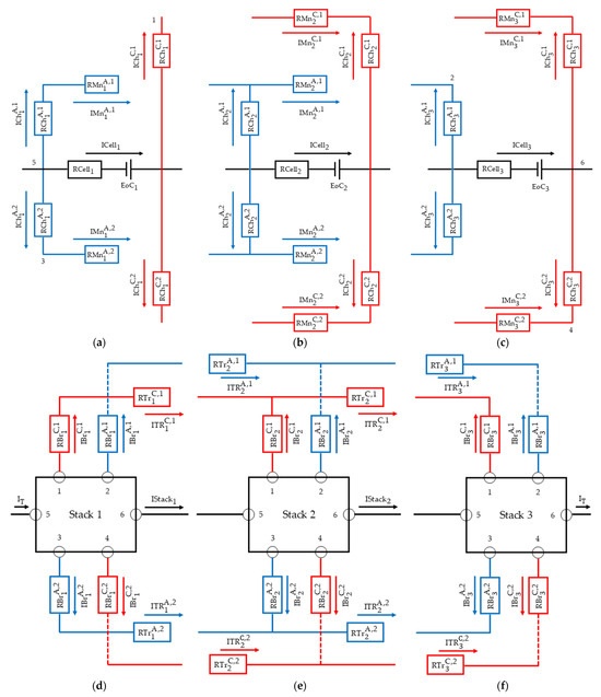
Figure 1.
Electrical circuit formation patterns between cells (a–c) and between stacks (d–f). The connections between the branches of the stacks and the cells are indicated by numbers. (a) First cells of stacks; (b) middle cells of the stacks; (c) last cells of stacks; (d) first stack of the battery; (e) middle stacks of the battery; (f) last stack of the battery.
From this analysis, 9 different cases are identified, each one introducing different unknowns, variables, and equations to the equation system (Table 1). The difference between the case of the first cell of the circuit and that of the first cell of the stack is that, in the equations of the first cell of the circuit, there is no dependence on variables from cells prior to it. There is no difference between the case of the last cell in the circuit and the last cell in the stack. They were simply differentiated to homogenize the implementation. There is a special case, related to the configuration of having a single stack. This case differs in that the stack does not add additional nets or nodes, and therefore, it does not add additional variables, unknowns, and equations.

Table 1.
Variables, unknowns, and equations of the identified cases.
In this analysis, only one configuration has been discarded, which is that of the stacks having a single cell, because it has not been seen to make much practical sense.
4.2. Analyzing the Equation System: Matrix Indexing
The equation system must be converted to matrix form for solution by computer. This way, two column vectors (A and I) and a rectangular matrix (B) are defined, fulfilling the equality shown in Equation (1):
where A is a column vector with the independent terms of the system of equations, B is a matrix with the coefficients of the equations of the system, and I is a column vector with the unknowns of the system (the currents). The values of the unknowns are obtained by premultiplying by the inverse of B on both sides. In order to generate these matrices, it is necessary to define how they will be organized. It was decided to index the matrices in such a way that the unknowns of the instances of the cases are contiguous in vector I. Table 2 serves as an example of indexing vector I for a case with 4 stacks of 3 cells each.
Table 2.
Example of the indexing of the vector for a case with 4 stacks and 3 cells for each stack.
Each row of matrix B follows the same indexing as the column vector I. The equations of each case instance are entered one by one, in an orderly manner, into each row of the A and I vectors as well as the B matrix. First, the equations related to the nodes are entered and then those related to the nets. Thus, vector A is indexed as shown in Table 3 for the example case of Table 2.
Table 3.
Example of indexing vector for a case with 4 stacks and 3 cells for each stack.
The first number in the parenthesis refers to the stack number and the second to the cell number within that stack. In the previous indexing tables, it has not been specified in this way because the indexing of each case instance refers to the variables of its own case. The difference in this table is that the instances of the stack cases refer to variables specific to the cells.
4.3. Implementation
4.3.1. Particularities of Implementation
The implementation has been approached using object orientation. This is because the problem to be solved fits very well with this paradigm. The programming has been implemented with MATLAB 2023b. While MATLAB is ideal for both computation and modeling, MATLAB’s object orientation has some peculiarities that have affected implementation, making it a bit strange in some parts. To list some of these particularities:
- By default, objects are passed by value and not by reference; to be passed by reference, it is necessary that the classes of such objects inherit from a special MATLAB class [19].
- In the classes, you can specify the type of attributes and parameters. Although this is not necessary, it increases the robustness of the code and is useful at the time of programming.
- There is no such thing as null as in other programming languages. When specifying the attributes of the class, you can assign a value directly that serves as a default value of the attribute when creating the objects [20]. If nothing is specified, the attribute will default to a specific value. For example, for numerical array-type attributes, the default value is an empty array. For singular class types, as long as the constructor of the class can accept 0 parameters, the default is an object of that class calling the constructor with 0 arguments.
- It is possible to specify static methods, but not static attributes.
- However, the default value of attributes whose type is of an object class that is shared by all objects of that class. If at any time in the life of the object of the class the instance of that attribute is not replaced, all the objects will be operating with a shared attribute between them.
If you want to make a linkedlist-type structure specifying the type of attributes of the nodes that make references to other nodes, things get complicated. If you want to make classes that have attributes that are of a type of an abstract class, you have to specify as default value an instance of a non-abstract subclass of that class. For these reasons, what will be presented will be generic and the particularities introduced by MATLAB will be ignored. What we want to show is a way to deal with problems of this type, rather than the specific code of a programming language.
4.3.2. Class Definition
Each different case has been coded as a different class. Two superclasses are defined, to define the common interfaces of the classes related to cells and those related to stacks. Both cells and stacks can be viewed as nodes, which can be connected to two other nodes of the same type. Therefore, both the superclass—from which the classes relative to the cases of the stacks are derived—and the superclass—from which the relative cases of the cells are derived—are also derived from a superclass in which the behavior of a node as described above is implemented. In this way and roughly obviating implementation details, Figure 2 would show a diagram of the proposed hierarchy.
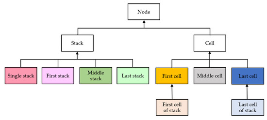
Figure 2.
Proposed class hierarchy diagram.
Each case class stores statically as constants the number of node and net equations, as well as indexes relative to the indexation of its variables for the rows of the matrix and the column of vector . There is no need to differentiate one set of variables for the indexing of the resistance coefficients for matrix and another for the currents of column vector , since both indexing processes follow the same pattern. The class instances, because they have node behavior, store a variable to reference the previous node and another to reference the next node.
Stacks have been seen as lists of cells. Therefore, additionally and as implemented, each instance of a Stack-type class has a variable referencing the first cell of the stack and another one referencing last cell. As stated, there are some equations in the first and last cells that change depending on whether the battery has more than one stack. If you want to delegate that change to the cell classes in those cases, you will have to add an extra reference referencing the stack to which it belongs. In this case, we wanted to delegate that to the classes related to the stacks; therefore, it would not be necessary (although we did include them in the implementation).
In an auxiliary mode, the stack instances also store the number of cells included in the stack itself as well as the number of unknowns added by those cells; these two attributes are necessary when coding the net equations of the stacks. Figure 3 shows a diagram to show what navigability would look like for a specific example.
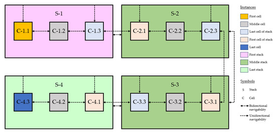
Figure 3.
Navigability diagram for an example of 4 stacks and 3 cells per stack.
In addition to these classes, there is another additional class that represents the list of stacks of the battery and that following the linkedlist model used so far has references to the instances of the first stack and the last stack of the battery or of the only stack in case there is only one.
In the Stack superclass, two attributes have been added, corresponding to two vectors, one of them being related to electrical resistance values and the other related to current values. For the Cell superclass, 4 attributes have been added, corresponding to two vectors; one for the electrical resistances and the other for the currents. The remaining two are to store the cell’s EoC value and the voltage value. The size of the arrays as well as their indexing are delegated to the classes that inherit from these superclasses and serve to store the inputs for encoding the equation system and the outputs for solving it.
4.4. Algorithms
The four main operations of this part are the creation of the data structures, the encoding of the node equations, the encoding of the net equations, and the decoding of the current vector results. All methods are started in the stack list instance.
4.4.1. Creation of the Data Structures
The creation of the data structures is where all instances of both stacks and cells are initialized, creating the double-linked list. Algorithm 1 shows the method in which the stacks are created from the stack list instance. In the constructors of all types of stacks, the construction of the intermediate cells is delegated to a method implemented in the generic superclass, as shown in Algorithm 2. Note that the setNext method shown in the algorithms generates the navigability in both directions, i.e., the reference of the next one is stored in the object in which it is invoked and the reference of the previous one is also stored in the instance that is passed as a parameter.
| Algorithm 1. Algorithm of stacks list construction. | ||||||||||
| Input: sNum: the number of stacks, cPsNum: the number of cells per stack. | ||||||||||
| Result: Build the double linked list of stacks and cells. | ||||||||||
| Class the method belongs to: StackList. | ||||||||||
| 1: | procedure buildStackList (sNum, cPsNum) | |||||||||
| 2: | self.stackNumber = sNum; | |||||||||
| 3: | if sNum == 1 | |||||||||
| 4: | self.fStack = SingleStack (cPsNum); | |||||||||
| 5: | self.varNum = 9∙cPsNum − 4; /** Each cell individually contributes 4 variables (4 channel currents and 1 cell current). In addition, the manifold currents must be taken into account. The total number of manifolds in a stack equals to The total number of manifolds in a stack of cells is equal to 4 × (number of cells − 1). A single stack does not add any more variables to the system, so the total number of variables is n × (4 + 1) + 4 × (n − 1) = 9n − 4 with n being the number of cells of the stack. **/ | |||||||||
| 6: | else | |||||||||
| 7: | self.fStack = FirstStack (cPsNum); | |||||||||
| 8: | tmpS = self.fStack; | |||||||||
| 9: | for i = 1: (sNum − 2) | |||||||||
| 10: | mStack = MiddleStack (cPsNum); | |||||||||
| 11: | tmpS.setNext (mStack); | |||||||||
| 12: | tmpS = mStack; | |||||||||
| 13: | end | |||||||||
| 14: | self.lStack = LastStack (cPsNum); | |||||||||
| 15: | tmpS.setNext (self.lStack); /** In case there are 0 middle stacks tmpS will refer to the object relative to the first stack. In case of having one or more middle stacks tmpS will refer to the object relative to the last middle stack **/ | |||||||||
| 16: | self.varNum = sNum∙ (9∙cPsNum + 4) − 4; /** It must be taken into account that each stack adds 9n − 4 variables relative to the cells. As there is more than one, each stack adds 4 variables (the branch currents), and in addition to that, the trunk currents must be taken into account. As with the manifolds, the total number of trunks is equal to 4 × (number of stacks − 1). Where m is the number of stacks and n is the number of cells per stack, the total number of variables is m × (9n − 4) + 4m + 4 × (m − 1) = m × (9n + 4) − 4. **/ | |||||||||
| 17: | end | |||||||||
| 18: | end | |||||||||
| Algorithm 2. Algorithm of the generic construction of the stacks. | ||||||||
| Input: fCell: instance of the first cell of the stack, lCell: instance of the last cell of stack, mCellNum: number of middle cells to be created. | ||||||||
| Result: Build the internal linked list of cells of each stack. | ||||||||
| Class the method belongs to: Stack. | ||||||||
| 1: | procedure buildStackCells (fCell, lCell, mCellNum) | |||||||
| 2: | self.fCell = fCell; | |||||||
| 3: | tmpC = self.fCell; | |||||||
| 4: | for i = 1: mCellNum | |||||||
| 5: | mCell = MiddleCell (); | // Create the middle cell objects. | ||||||
| 6: | tmpC.setNext (mCell); | |||||||
| 7: | tmpC = mCell; | |||||||
| 8: | end | |||||||
| 9: | self.lCell = lCell; | |||||||
| 10: | tmpC.setNext (self.lCell); /** Same as tmpS but with objects relative to cells. **/ | |||||||
| 11: | end | |||||||
The generic method receives as the parameter the instances of the first and last cell of the stack, due to the type differentiation between the first and last cell of the circuit and the first and last cell of the stack.
4.4.2. Codification of Node Equations
The node equations refer to the structure of the electrical circuit. The coefficients of these equations are always 1 or 0 and do not change as long as the circuit is not changed. Therefore, it is only necessary to run the coding process of these equations once, regardless of the simulation time imposed and the simulation steps to be performed. As explained above, the execution of the operations always starts in the stack list instance.
This instance has 3 additional attributes: An instance of an object that serves as an equation pointer, which refers to the row of the matrix or vector in which to encode the equations; an instance of an object that serves as a stack pointer, referring to the previous stack processed, the current stack to be processed and the next stack to be processed; and an instance of an object that, being of the same type as the stack pointer, serves to reference the previous cell processed, the current cell to process, and the next cell to process. These two pointers do not refer to the objects itself. What they do is reference with the absolute position number the first variable/unknown that introduces the case of the object in the equation system.
Algorithm 3 shows the method of how the stack list instance starts the process of encoding the node equations.
| Algorithm 3. Algorithm for the codification of the node equations (I) | |||||||
| Input: bMat: equation system coefficient matrix. | |||||||
| Result: Encode of the equations of stacks and cells nodes. | |||||||
| Class the method belongs to: StackList. | |||||||
| 1: | procedure buildNodeEquations (bMat) | ||||||
| 2: | self.eqPntr.reset (1); /** Reset pointer to point to row 1 of matrix and vectors. **/ | ||||||
| 3: | self.cPntr.reset (1); /** Reset the object so that the index indicating the absolute position of the first variable of the next cell to be processed is equal to 1. **/ | ||||||
| 4: | tmpS = self.fStack; | ||||||
| 5: | self.sPntr.reset (1 + tmpS.cellVarNumber); /** Reset the object so that the index indicating the absolute position of the first variable of the next stack to be processed is equal to the number of cell variables of the first stack + 1. **/ | ||||||
| 6: | for i = 1:self.stackNumber | ||||||
| 7: | tmpS.buildNodeEquations (bMat, self.cPntr, self.sPntr, self.eqPntr); /** Call to the generic method of Stack type objects that is implemented in the Stack superclass. **/ | ||||||
| 8: | self.eqPntr.updtRowPntr (tmpS.netEquationsNumber); /** The pointer is updated each time a cell or stack equation is encoded. However, since the node and net equations of each cell/stack are encoded contiguously and this method only encodes node equations, it is necessary to update the pointer after processing each stack to omit the rows relating to the net equations of that stack. **/ | ||||||
| 9: | tmpS = tmpS.getNext (); | ||||||
| 10: | end | ||||||
| 11: | end | ||||||
The first thing that is performed in the method is the reset of the positions to which the pointers point, returning them to the starting positions. After that, it enters a loop in which, for each stack, the buildNodeEquations method is invoked. Keep in mind that, as with the variables, the equations of each case are codified sequentially in the matrix and vectors, so that if a case introduces a total of 7 equations to the system (counting the equations of nodes and nets), these 7 will be coded in contiguous rows. Since, in this method, only the equations of the nodes of the cases are being codified, it is necessary to adjust the equation pointer to omit the rows relative to the equations of the nets after processing each case, which is why the updtRowPntr method is invoked. Algorithm 4 has been implemented for the buildNodeEquations method of the stacks.
| Algorithm 4. Algorithm for the codification of the node equations (II) | |||||||
| Input: bMat: equation system coefficient matrix, cPntr: cell pointer, sPntr: stack pointer, eqPntr: equation pointer. | |||||||
| Result: Encode the equations of stack and their cells nodes. | |||||||
| Class the method belongs to: Stack. | |||||||
| 1: | procedure buildNodeEquations (bMat, cPntr, sPntr, eqPntr) | ||||||
| 2: | self.updatePointerIndexes (sPntr); /** Call to the Stack type object’s own method to update the stacks variable pointer. Each subclass of Stack implements this method. For objects relative to the first and middle stacks the implementation is the same, but for objects relative to the last stack it differs. **/ | ||||||
| 3: | tmpC = self.fCell; | ||||||
| 4: | for i = 1:self.cellNumber | ||||||
| 5: | tmpC.buildNodeEquations (bMat, cPntr, eqPntr); /** Call to the generic method of Cell type objects implemented in the Cell superclass. **/ | ||||||
| 6: | eqPntr.updtRowPntr (tmpC.netEquationsNumber); /** The same commented about the equation pointer in Algorithm 3 but applied to the context of cell equations. **/ | ||||||
| 7: | tmpC = tmpC.getNext (); | ||||||
| 8: | end | ||||||
| 9: | self.stackConnector.connect (self, bMat, sPntr, eqPntr); /** To complete the equations relating to the nodes that connect the stack to the first and last cell. It could have been implemented in the classes related to those objects. But doing so would mean losing the generalization of the implementation of the first and last cells in the case of there being only one stack. It was decided to create our own objects to carry out this implementation, to make it possible to have it generalized in case we wanted to implement other ways of connecting the stacks with the cells. **/ | ||||||
| 10: | self.buildSelfNodeEquations (bMat, sPntr, eqPntr); /** Call to the Stack type object’s own method to encode the equations relative to the stack. Each subclass of Stack implements this method. **/ | ||||||
| 11: | end | ||||||
The updatePointerIndexes and buildSelfNodeEquations methods have their implementation delegated to the subclasses of the Stack class. As mentioned earlier in the article, some equations of the first and last cells are modified in case there is more than one stack. In addition, the equations that are affected depend on how the stacks are connected to their cells (u-form or z-form, for example). To solve this peculiarity, we have assigned as an attribute (named as stackConnector) to the Stack class an object type to delegate the modification of these equations. As this work is oriented towards stacks connected in the form of z, we have ensured that these objects are created in the constructors. But in cases of allowing other types of connections, it would be an input parameter of the constructor or another function of the Stack-derived classes. The class relative to the case of having only one stack would have an object of this type, which would not perform any action. As with the Stack-derived classes, the updatePointerIndexes and buildNodeEquations of the Cell class have delegated implementations in the subclasses of Cell. This way, it is only necessary to differentiate cases in the construction of the data structures. The method buildNodeEquations of the Cell classes has the form shown in Algorithm 5.
| Algorithm 5. Algorithm for the codification of the node equations (III). | ||||
| Input: bMat: equation system coefficient matrix, eqPntr: equation pointer, cPntr: cell pointer. | ||||
| Result: Encode of cell node equations. | ||||
| Class the method belongs to: all types of Cell. | ||||
| 1: | procedure buildNodeEquations (bMat, cPntr, eqPntr) | |||
| 2: | self.updatePointerIndexes (cPntr); | |||
| 3: | self.buildEq1 (bMat, cPntr, eqPntr); | |||
| 4: | eqPntr.updtRowPntr (1); | |||
| 5: | self.buildEq2 (bMat, cPntr, eqPntr); | |||
| 6: | eqPntr.updtRowPntr (1); | |||
| 7: | // … Repeat to all node equations of the cell | |||
| 8: | end | |||
Equation (2) is the first equation of the case relative to the first cell of the stacks.
This equation is encoded in the matrix as shown in Algorithm 6. The coding of the equations relative to the nodes have the same form.
| Algorithm 6. Example algorithm of coding of Equation (2) relative to the case of first stack cell. | ||||
| Input: bMat: equation system coefficient matrix, eqPntr: equation pointer, cPntr: cell pointer. | ||||
| Result: Encode the first equation of the first cell of a stack. | ||||
| Class the method belongs to: FirstCellOfStack. | ||||
| 1: | procedure buildEq1 (bMat, cPntr, eqPntr) | |||
| 2: | bMat.setValue (eqPntr.row, cPntr.prevIdx + self.previous.Cell, 1); | |||
| 3: | bMat.setValue (eqPntr.row, cPntr.prevIdx + self.previous.ChC1, −1); | |||
| 4: | bMat.setValue (eqPntr.row, cPntr.prevIdx + self.previous.ChC2, −1); | |||
| 5: | bMat.setValue (eqPntr.row, cPntr.actIdx + self.Cell, −1); | |||
| 6: | bMat.setValue (eqPntr.row, cPntr.actIdx + self.ChA1, −1); | |||
| 7: | bMat.setValue (eqPntr.row, cPntr.actIdx + self.ChA2, −1); | |||
| 8: | end | |||
Before each stack or cell instance processing, the corresponding pointer instance is updated. Remembering that these pointers store the absolute value of the first variable of the previous case processed, the current case processed and the next case to be processed, the update is performed as follows in Table 4.
Table 4.
Update example of the cell and stack pointers.
That is, the values are shifted to the left to adjust them to the current case to be processed. Since this method is invoked before and not after processing the instance, in the method to reset the pointers, the position of the first instance to be processed is passed as a value but stored as the next instance to be processed. Table 5 shows an example of the modification of the stack and cell pointers for a battery with 4 stacks and 3 cells per stack. This method of updating the pointers is the same as the coding of the equations of the nodes and nets.
Table 5.
Full example of the update of the stack and cell pointers.
4.4.3. Codification of Net Equations
The algorithmizing of the coding of the equations of the nets has been performed in a very similar way to that of the equations of the nodes. This is no coincidence, as it is precisely what was sought. In this way, the mechanisms used for the coding of the node equations could be reused.
Unlike with the node equations, to codify the net equations, additional inputs are needed, relating to the EoC values of each cell as well as the resistances of each pipe segment. These inputs could be considered as inputs to the methods related to the coding of the equations. However, doing so was problematic. This is because introducing the values as inputs, given that these inputs contain arrays with the values of the resistors and EoC, implied that it was necessary to know from the outside how the electrical circuit is generated and to have such arrays generated by differentiating the cases. This same problem manifested itself with the output.
It was therefore decided to associate the Cell and Stack objects with the inputs and outputs, making each object have attributes to receive the inputs and return the outputs. These attributes are lists of objects and not double-type values. In this way, the reference to those objects is stored not only internally in the case objects (Cell- and Stack-type objects), but also in an ordered way, in an external object. The same applies for current vectors and voltage variables. This makes it possible to externally modify the values without having to iterate over the objects related to the cases. Although not detailed, the construction of the external arrays is part of the construction of the data structures. Figure 4 shows a schematic of the above.
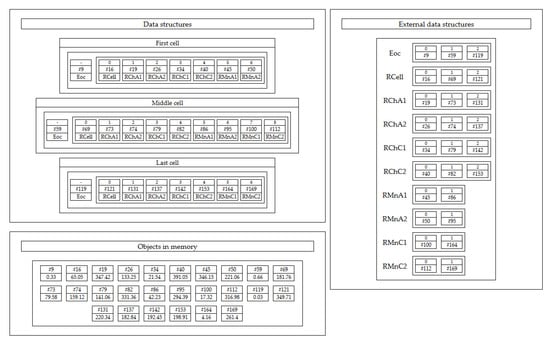
Figure 4.
Diagram of the organization of the inputs (the outputs follow the same logic).
This is the major difference in how the coding of the net equations has been performed with respect to those of the nodes, with the rest being very similar. Algorithm 7 presents how to start coding the net equations in the StackList object type. As can be seen, the structure of Algorithm 3 is maintained.
| Algorithm 7. Algorithm for the codification of the net equations (I). | ||||||||
| Input: aVec: equation system column vector of the independent term, bMat: equation system coefficient matrix, current: imposed current to the battery. | ||||||||
| Result: Encode of the equations of stacks and cells nets. | ||||||||
| Class the method belongs to: StackList. | ||||||||
| 5: | procedure buildNetEquations (aVec, bMat, current) | |||||||
| 6: | self.eqPntr.reset (1); | /** The same resets are performed as in the function buildNodeEquations of the same class. **/ | ||||||
| 7: | self.cPntr.reset (1); | |||||||
| 8: | tmpS = self.fStack; | |||||||
| 9: | self.sPntr.reset (1 + tmpS.cellVarNumber); | |||||||
| 10: | aVec.setValue (eqPntr.row, 1, current); /** Assign in row 1 of the column vector A the value of the current. In the call to the function the position of the column is also specified even if there is only one column. **/ | |||||||
| 11: | for i = 1:self.stackNumber | |||||||
| 12: | tmpS.buildNetEquations (aVec, bMat, self.cPntr, self.sPntr, self.eqPntr); /** This time the equation pointer update is made in the stack object. This is because when processing the nodes, the equation pointer is located in the first row relative to the stack net equations. However, when the stack net equations are processed, the equation pointer is located in the first row relative to the first node equation of the first cell of the next stack. **/ | |||||||
| 13: | tmpS = tmpS.getNext (); | |||||||
| 14: | end | |||||||
| 15: | end | |||||||
Apart from the method calling for stack objects, the only difference with respect to that shown in Algorithm 3 is that the equation pointer is not updated. This update is performed inside the method that was called for in the loop. Algorithm 8 shows the method related to the encoding of the equations of the net of stack-type objects.
| Algorithm 8. Algorithm for the codification of the node equations (II). | |||||||
| Input: aVec: equation system column vector of the independent term, bMat: equation system coefficient matrix, cPntr: cell pointer, sPntr: stack pointer, eqPntr: equation pointer. | |||||||
| Result: Encode the equations of stack and their cells nets. | |||||||
| Class the method belongs to: Stack. | |||||||
| 5: | procedure buildNetEquations (aVec, bMat, cPntr, sPntr, eqPntr) | ||||||
| 6: | self.updatePointerIndexes (sPntr); | ||||||
| 7: | tmpC = self.fCell; /** In the processing of the stack net equations, as with the nodes, the net equations of the stack cells are first encoded. **/ | ||||||
| 8: | for i = 1:self.cellNumber | ||||||
| 9: | eqPntr.updtRowPntr (tmpC.nodeEquationsNumber); /** Since the equation pointer is located in the row of the first cell node equation, it should be updated to be located in the row of the first cell net equation. **/ | ||||||
| 10: | tmpC.buildNetEquations (aVec, bMat, cPntr, eqPntr); | ||||||
| 11: | tmpC = tmpC.getNext (); | ||||||
| 12: | end | ||||||
| 13: | eqPntr.updtRowPntr (self.nodeEquationsNumber); /** At the end of the loop, the same thing happens with the equation pointer as happened in the loop. Therefore, it is updated to place it in the row of the first net equation of the stack. **/ | ||||||
| 14: | self.buildSelfNetEquations (aVec, bMat, cPntr, sPntr, eqPntr); | ||||||
| 15: | end | ||||||
4.4.4. Decoding the Current Vector
After performing the operation of the inverse of B and premultiplying vector A with this matrix, it is simply necessary to perform a complete iteration of the cell and stack objects to obtain the values of the currents of vector I using the indices. The output values are stored in the objects relative to the outputs of each Cell and Stack object, so that they are accessible from the outside.
5. Comparative Experiments
This section is dedicated to validating the implementation of the algorithm. Since we do not have our own experimental data, comparisons will be made using the parameters of other papers and their results with what is obtained with our model.
5.1. First Comparison
A test of the model has been performed using the design parameters G of [12] and comparing the results. The parameters of model G of item [12] are shown in Table 6.
Table 6.
Parameters for comparison 1.
Figure 5 shows a comparison between the shunt current data obtained by the model and the data shown in the article [12].
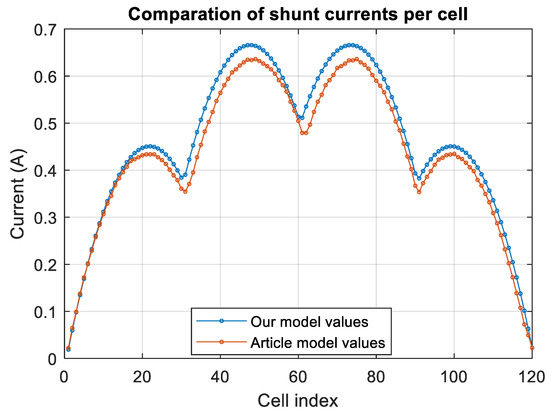
Figure 5.
Comparison using the G design of [12].
The data of the article with which the comparison has been made were obtained from the image shown in that article, so they are not entirely accurate with respect to what was obtained in the article from which they were taken. The shape of the graph is the same, although there are differences in the values obtained. We would have liked to understand the reason for this difference, but the article itself does not show the model. That said, the differences are not too significant.
5.2. Second Comparison
The second comparison has been made with the case relative to the discharge of 54A with SoC 0.5 of article [8]. Having analyzed the data given in the article, the following parameterization has been extracted (Table 7).
Table 7.
Parameters for comparison 1.
As with the previous comparison, the data with which they are compared have been extracted using the graphs shown in the article. In addition, these data have also been necessary for the obtaining of some of the parameters (cell’s EoC, for example). Figure 6 shows the comparison of the cell currents and voltages obtained by our model and the one obtained in [8] for a discharge current of 54 amps and a SoC of 0.5.
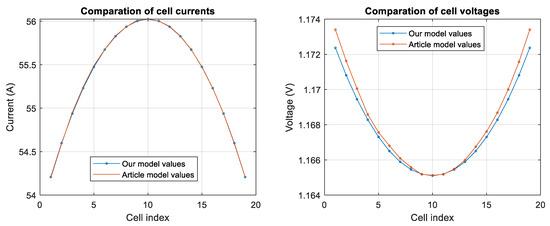
Figure 6.
Comparison with the data of article [8] for 54 amperes of discharge current and a SoC 0.5.
6. Analysis
This part is dedicated to the analysis of the implementation execution times. The program runs have been executed on a computer with 16 Gb of ram and an Intel(R) Core (TM) i5-7500 processor. When measuring times, a differentiation has been established between the part in which the objects are constructed together with the codification of the node equations and the part in which the mesh equations are encoded and the system is solved. The execution of the codification of the node equations is performed after the construction of the objects in the same call, so they are measured together. To measure the times, the functions for constructing the objects (together with the codification of the node equations) and the function for codification the net equations and solving the equation system have been executed in a loop. Table 8 shows the results for different parameterizations of stack number and cell number per stack. The times shown have been obtained by executing loops of 100 iterations except in the last cases, in which it has been decided to reduce the number of repetitions to 20.
Table 8.
Execution times of different cases.
Figure 7 is a graphical representation of the data obtained.
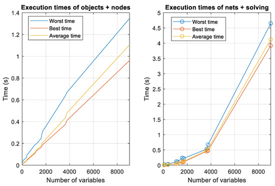
Figure 7.
Graphical representation of case execution times.
As can be seen, the times relative to the instantiation of the objects, together with the codification of the equations of the nodes, follow a fairly linear pattern, for the codification of the net equations and the resolution of the equation system is different as the number of variables increases. This is to be expected, since to solve the system of equations, the calculation of the inverse of a matrix of dimensions equal to the number of variables must be performed.
As previously mentioned, before addressing the problem in the manner shown in the article, a code was implemented which, based on the parameters of the number of stacks and cells per stack, carried out the construction of the equivalent circuit in Simulink. The problem with that is that the model compilation times were already very high, with the order of hours for a cell count at around 120. Once compiled, execution was also very slow, which is why these results are very positive.
Finally, it is worth highlighting the linearity with respect to the number of variables with which the times of object creation increase, not to mention the introduction of the coefficients of the node equations. This was something to be expected, since, in the end, the algorithms are linear. However, in the times relative to the insertion of the coefficients of the net equations and the resolution, this linearity does not exist, because an inverse of a matrix is performed in the resolution.
7. Conclusions
This work arises from the need to model the shunt currents of a generic vanadium flow redox battery. While there are quite a few articles that discuss modeling shunt currents, many of them make simplifications that limit the possibility of testing different hypothetical cases. In addition, none of the articles consulted by the authors on this topic showed how they had carried out the implementation, possibly due to its complexity, the use of external tools to simulate, or that they have only been able to carry out the implementation for a specific case.
This article has shown a way to implement the resolution of shunt currents in a generic way for batteries with any number of cells and stacks (except for the special case of one cell per stack, since it was thought that it did not make much sense). The factors to be taken into account and the patterns that must be identified in order to be able to reach implementation have been discussed.
Author Contributions
Conceptualization, D.A.I.-G.; methodology, D.A.I.-G.; software, validation, D.A.I.-G.; formal analysis, D.A.I.-G.; investigation, D.A.I.-G.; resources; data curation; writing—review and editing, D.A.I.-G. and J.M.L.-G.; visualization; supervision; project administration, E.Z. and J.O.; funding acquisition, E.Z. All authors have read and agreed to the published version of the manuscript.
Funding
Mobility Lab Foundation, a governmental organization of the Provincial Council of Araba and the local council of Vitoria-Gasteiz.
Data Availability Statement
All data generated in the current study are available upon reasonable request to the corresponding authors.
Conflicts of Interest
Javier Olarte is employed by the Center for Cooperative Research on Alternative Energies (CIC EnergiGUNE). The remaining authors declare that the research was conducted in the absence of any commercial or financial relationships that could be construed as potential conflicts of interest.
Appendix A
This appendix is dedicated to showing the equations of the equivalent electric circuit by organizing them as shown in the analysis of the electric circuit formation. The authors have previously published the model in a more detailed form in another journal [21].
Appendix A.1. Equations of the First Cell of the Stack and the First Cell of the Circuit
The Equations (A1)–(A7) are those relative to the first cell of the stacks.
The first cell of the circuit is a particular case of the first cell of a stack. In this case, the application of Equation (A1) is replaced with that of Equation (A8):
where is the current imposed in the charge or discharge of the battery. In this case, the possibility of the battery having only one stack is also considered, replacing Equations (A3) and (A4) with Equations (A9) and (A10) due to the disappearance of the trunks and branches that join stacks.
Appendix A.2. Equations of Middle Cells of Stacks
The Equations (A11)–(A19) are those relative to the intermediate cells of the stacks.
These equations are not affected by the number of battery stacks.
Appendix A.3. Equations of Last Cell of the Stack and Last Cell of the Circuit
The Equations (A20)–(A26) are those relative to the last cells of the stacks.
Just as it happened with the first cell of the circuit, the last cell of the circuit is a particular case of the last cell of the stack. The equations that apply to this particular case are similar to all the previous ones, except if the battery has a single stack, the Equations (A21) and (A24) would be replaced with the Equations (A27) and (A28).
Appendix A.4. Equations of the First Stack of the Circuit
The Equations (A29)–(A34) are those relative to the first stack of the circuit.
Appendix A.5. Equations of the Middle Stacks of the Circuit
The Equations (A35)–(A42) are those relative to the middle stacks of the circuit.
Appendix A.6. Equations of Last Stack of the Circuit
The Equations (A43)–(A48) are those relative to the last stack of the circuit.
Appendix A.7. Equations of Single Stack
In the case that the battery has only one stack, the considerations made for the first and last cells of the circuit must be taken into account. Otherwise, no additional equations are added.
References
- Li, Y.; Skyllas-Kazacos, M.; Bao, J. A Dynamic Plug Flow Reactor Model for a Vanadium Redox Flow Battery Cell. J. Power Sources 2016, 311, 57–67. [Google Scholar] [CrossRef]
- Trovò, A.; Picano, F.; Guarnieri, M. Maximizing Vanadium Redox Flow Battery Efficiency: Strategies of Flow Rate Control. In Proceedings of the 2019 IEEE 28th International Symposium on Industrial Electronics (ISIE), Vancouver, BC, Canada, 12–14 June 2019; pp. 1977–1982. [Google Scholar]
- Zhao, X.; Kim, Y.-B.; Jung, S. Shunt Current Analysis of Vanadium Redox Flow Battery System with Multi-Stack Connections. J. Energy Storage 2023, 73, 109233. [Google Scholar] [CrossRef]
- Xing, F.; Zhang, H.; Ma, X. Shunt Current Loss of the Vanadium Redox Flow Battery. J. Power Sources 2011, 196, 10753–10757. [Google Scholar] [CrossRef]
- Burney, H.S.; White, R.E. Predicting Shunt Currents in Stacks of Bipolar Plate Cells with Conducting Manifolds. J. Electrochem. Soc. 1988, 135, 1609. [Google Scholar] [CrossRef]
- Chou, H.-W.; Chang, F.-Z.; Wei, H.-J.; Singh, B.; Arpornwichanop, A.; Jienkulsawad, P.; Chou, Y.-S.; Chen, Y.-S. Locating Shunt Currents in a Multistack System of All-Vanadium Redox Flow Batteries. ACS Sustain. Chem. Eng. 2021, 9, 4648–4659. [Google Scholar] [CrossRef]
- Fink, H.; Remy, M. Shunt Currents in Vanadium Flow Batteries: Measurement, Modelling and Implications for Efficiency. J. Power Sources 2015, 284, 547–553. [Google Scholar] [CrossRef]
- Chen, Y.-S.; Ho, S.-Y.; Chou, H.-W.; Wei, H.-J. Modeling the Effect of Shunt Current on the Charge Transfer Efficiency of an All-Vanadium Redox Flow Battery. J. Power Sources 2018, 390, 168–175. [Google Scholar] [CrossRef]
- Tang, A.; McCann, J.; Bao, J.; Skyllas-Kazacos, M. Investigation of the Effect of Shunt Current on Battery Efficiency and Stack Temperature in Vanadium Redox Flow Battery. J. Power Sources 2013, 242, 349–356. [Google Scholar] [CrossRef]
- Trovò, A.; Marini, G.; Sutto, A.; Alotto, P.; Giomo, M.; Moro, F.; Guarnieri, M. Standby Thermal Model of a Vanadium Redox Flow Battery Stack with Crossover and Shunt-Current Effects. Appl. Energy 2019, 240, 893–906. [Google Scholar] [CrossRef]
- Darling, R.M.; Shiau, H.-S.; Weber, A.Z.; Perry, M.L. The Relationship between Shunt Currents and Edge Corrosion in Flow Batteries. J. Electrochem. Soc. 2017, 164, E3081. [Google Scholar] [CrossRef]
- Ye, Q.; Hu, J.; Cheng, P.; Ma, Z. Design Trade-Offs among Shunt Current, Pumping Loss and Compactness in the Piping System of a Multi-Stack Vanadium Flow Battery. J. Power Sources 2015, 296, 352–364. [Google Scholar] [CrossRef]
- Wandschneider, F.T.; Röhm, S.; Fischer, P.; Pinkwart, K.; Tübke, J.; Nirschl, H. A Multi-Stack Simulation of Shunt Currents in Vanadium Redox Flow Batteries. J. Power Sources 2014, 261, 64–74. [Google Scholar] [CrossRef]
- Prokopius, P.R. Model for Calculating Electrolytic Shunt Path Losses in Large Electrochemical Energy Conversion Systems. 1976. Available online: https://ntrs.nasa.gov/citations/19760014614 (accessed on 19 June 2025).
- Kaminski, E.A.; Savinell, R.F. A Technique for Calculating Shunt Leakage and Cell Currents in Bipolar Stacks Having Divided or Undivided Cells. J. Electrochem. Soc. 1983, 130, 1103. [Google Scholar] [CrossRef]
- Glazkov, A.; Pichugov, R.; Loktionov, P.; Konev, D.; Tolstel, D.; Petrov, M.; Antipov, A.; Vorotyntsev, M.A. Current Distribution in the Discharge Unit of a 10-Cell Vanadium Redox Flow Battery: Comparison of the Computational Model with Experiment. Membranes 2022, 12, 1167. [Google Scholar] [CrossRef] [PubMed]
- Trovò, A.; Alotto, P.; Giomo, M.; Moro, F.; Guarnieri, M. A Validated Dynamical Model of a kW-Class Vanadium Redox Flow Battery. Math. Comput. Simul. 2021, 183, 66–77. [Google Scholar] [CrossRef]
- Moro, F.; Trovò, A.; Bortolin, S.; Del Col, D.; Guarnieri, M. An Alternative Low-Loss Stack Topology for Vanadium Redox Flow Battery: Comparative Assessment. J. Power Sources 2017, 340, 229–241. [Google Scholar] [CrossRef]
- Comparison of Handle and Value Classes. Available online: https://www.mathworks.com/help/matlab/matlab_oop/comparing-handle-and-value-classes.html (accessed on 2 April 2025).
- Initialize Property Values. Available online: https://www.mathworks.com/help/matlab/matlab_oop/initialize-property-values.html#br18hyr (accessed on 10 February 2025).
- Ispas-Gil, D.A.; Zulueta, E.; Olarte, J.; Zulueta, A.; Fernandez-Gamiz, U. Optimization of the Shunt Currents and Pressure Losses of a VRFB by Applying a Discrete PSO Algorithm. Batteries 2024, 10, 257. [Google Scholar] [CrossRef]
Disclaimer/Publisher’s Note: The statements, opinions and data contained in all publications are solely those of the individual author(s) and contributor(s) and not of MDPI and/or the editor(s). MDPI and/or the editor(s) disclaim responsibility for any injury to people or property resulting from any ideas, methods, instructions or products referred to in the content. |
© 2025 by the authors. Licensee MDPI, Basel, Switzerland. This article is an open access article distributed under the terms and conditions of the Creative Commons Attribution (CC BY) license (https://creativecommons.org/licenses/by/4.0/).