Article

A Survey of Visual SLAM Based on RGB-D Images Using Deep Learning and Comparative Study for VOE

Information Technology Department, Tan Trao University, Tuyen Quang City 22000, Vietnam
*
Author to whom correspondence should be addressed.
Algorithms 2025, 18(7), 394; https://doi.org/10.3390/a18070394
Submission received: 21 April 2025 / Revised: 13 June 2025 / Accepted: 23 June 2025 / Published: 27 June 2025
(This article belongs to the Special Issue Advances in Deep Learning and Next-Generation Internet Technologies)

Abstract

Visual simultaneous localization and mapping (Visual SLAM) based on RGB-D image data includes two main tasks: One is to build an environment map, and the other is to simultaneously track the position and movement of visual odometry estimation (VOE). Visual SLAM and VOE are used in many applications, such as robot systems, autonomous mobile robots, assistance systems for the blind, human–machine interaction, industry, etc. To solve the computer vision problems in Visual SLAM and VOE from RGB-D images, deep learning (DL) is an approach that gives very convincing results. This manuscript examines the results, advantages, difficulties, and challenges of the problem of Visual SLAM and VOE based on DL. In this paper, the taxonomy is proposed to conduct a complete survey based on three methods to construct Visual SLAM and VOE from RGB-D images (1) using DL for the modules of the Visual SLAM and VOE systems; (2) using DL to supplement the modules of Visual SLAM and VOE systems; and (3) using end-to-end DL to build Visual SLAM and VOE systems. The 220 scientific publications on Visual SLAM, VOE, and related issues were surveyed. The studies were surveyed based on the order of methods, datasets, evaluation measures, and detailed results. In particular, studies on using DL to build Visual SLAM and VOE systems have analyzed the challenges, advantages, and disadvantages. We also proposed and published the TQU-SLAM benchmark dataset, and a comparative study on fine-tuning the VOE model using a Multi-Layer Fusion network (MLF-VO) framework was performed. The comparison results of VOE on the TQU-SLAM benchmark dataset range from 16.97 m to 57.61 m. This is a huge error compared to the VOE methods on the KITTI, TUM RGB-D SLAM, and ICL-NUIM datasets. Therefore, the dataset we publish is very challenging, especially in the opposite direction (OP-D) when collecting and annotation data. The results of the comparative study are also presented in detail and available.

1. Introduction

Localization and mapping of the environment (3D space) for robots operating in the home, autonomous vehicles in factories, and as guides for blind people are very important research in computer vision and robotics. In the study of Zhai et al. [1,2], machine learning was used to train the model to predict the robot’s motion trajectory and monitor the observation state. From there, applications can be developed to control the robot’s two arms.
These studies of Visual SLAM and VOE help entities locate themselves in the environment, understand the scene, and employ their navigation. To perform these tasks, it is necessary to solve computer vision problems. Previously, the input data used to perform the two problems Visual SLAM and VOE were SONAR sensors, 2D laser scanners, and LiDAR. In the 21st century, the development of computer hardware and image sensors has brought many newer and more affordable types of data such as monocular, stereo, or RGB-D. They can collect visual information about their surroundings. Therefore, research on Visual SLAM and VOE in studies on these types of data is receiving very strong research attention.
Recently, with the advent of DL with some popular model types such as Convolutional (conv.) Neural Networks (CNNs), Recurrent Neural Networks (RNNs), Generative Adversarial Networks (GANs), etc., these models have brought impressive results in computer vision, ML, and AI. Recent studies have investigated the following: Ajagbe et al. [3] conducted a survey of studies using DL for pandemic detection and prediction from 44 scientific publications on using DL for detection and prediction and related issues. The survey results were systematized and analyzed from data tables and charts in these 44 studies.
At the same time, the study also clearly shows the current status and forecast results of the COVID-19 pandemic. Adetayo et al. [4]) conducted a statistical survey and analyzed data collected from 145 stakeholders on the use of ML and AI technology in agricultural production in Shonga, Nigeria. The data collected were analyzed based on eleven factors, and shortcomings and limitations were also pointed out to find solutions to overcome these situations. Taiwo et al. [5] conducted a study applying ML and DL to predict crimes based on hourly activities on Twitter and existing criminal profiles based on demographics. The features were extracted from the data and trained based on the SHAP model. The xgboost algorithm was used to optimize the model during the model training. The accuracy result of the model was 81%.
In recent years, there have been many valuable surveys on visual SLAM and VOE, as shown in Table 1. The input data for the studies surveyed above were derived solely from image sensors, and DL was also the method, with the best results in studies on Visual SLAM and VOE. A study by Abaspur et al. [6] presented a complete survey of Visual SLAM methods, in which the Visual SLAM construction model includes five steps (feature extraction, feature matching, pose estimation, loop closure, and map building), as shown in Figure 1. The study of Favorskaya et al. [7] is the most recent survey of Visual SLAM, in which the Visual SLAM process includes two main stages: VOE and loop closure. When broken down in detail, it includes six steps: data pre-processing, feature extraction, feature matching, pose estimation, map building, and loop closure. Recently, Phan et al. [8] proposed a detailed survey of DL methods for VOE, including DL networks in each module of the VOE system and end-to-end DL for VOE. In addition, the authors also focused on the loss functions of DLs for VOE model optimization.
DL is also examined with three methods to implementing Visual SLAM: adding auxiliary modules based on DL, replacing modules with DL modules, and using end-to-end DL. However, most of the above surveys are based on statistics and classification of methods and datasets without examining in detail the algorithms and results of Visual SLAM and VOE methods. At the same time, the advantages, disadvantages, and challenges of implementing Visual SLAM and VOE have not been presented. However, DL requires a large amount of learning data, especially to have a model capable of estimating environmental maps in many different environments and contexts, enriching learning data is an urgent requirement. Building a dataset to evaluate Visual SLAM and VOE algorithm models faces many challenges such as large environments with difficulties in collecting and synchronizing data, data collection equipment, annotation data, and labeling data, as well as external factors affecting the data collection process. Previous datasets such as the KITTI [9,10,11], TUM RGB-D SLAM [12], and ICL-NUIM [13] datasets have been collected and used to evaluate models for nearly a decade; these databases were collected from image sensors based on old technology, such as TUM collected and synchronized based on Microsoft Kinect. Therefore, collecting databases to evaluate Visual SLAM and VOE algorithmic models is necessary.
Table 1. Surveys on the Visual SLAM and VOE from 2017 to 2024.
AuthorsYearMethodsType of
Datasets
Survey
of DL
[14]2017Visual SLAM,
VOE
RGB-DNo
[15]2019Visual-inertial
SLAM,
VOE
Stereo,
RGB-D
No
[16]2020Visual SLAM,
VOE
RGB-DYes
[17]2020Visual SLAMRGB-DYes
[18]2020Semantic SLAM,
Visual SLAM
Monocular,
RGB-D,
Stereo
Yes
[19]2021Visual SLAMRGB-DYes
[20]2022Embedded SLAM,
Visual-inertial
SLAM,
Visual-SLAM,
VOE
RGB-DYes
[6]2022Visual SLAM,
VOE
Sonar,
Laser,
LiDAR,
RGB-D,
Monocular,
Stereo
Yes
[21]2022Visual SLAMRGB-DYes
[22]2022Visual SLAMRGB-DYes
[23]2022Visual SLAM,
VOE
RGB-DYes
[24]2022Semantic
Visual SLAM
Sonar,
Laser,
LiDAR,
RGB-D,
Monocular,
Stereo
Yes
[25]2022Visual SLAM,
VOE
RGB-D,
GPS
No
[26]2022Visual SLAMRGB-DYes
[27]2022VOELiDAR,
RGB-D,
Point cloud
Yes
[28]2023Visual SLAM,
VOE
RGB-DYes
[29]2023Visual SLAMMonocular,
RGB-D,
Stereo
Yes
[7]2023Visual SLAM,
VOE
Monocular,
RGB-D,
Stereo
Yes
[30]2024Visual SLAM,
VOE
Monocular,
RGB-D
Yes
[31]2024Visual SLAM,
VOE
Monocular,
RGB, Stereo,
LiDAR
No
[32]2024Visual SLAM,
Visual-Inertial SLAM
RGB-D, IMUNo
[33]2024Visual SLAM,
Visual-Inertial SLAM
RGB-DYes
[34]2024VOEMonocular,
RGB
Yes
Although there have been surveys on DL-based Visual SLAM and VOE, these surveys only cover one aspect such as surveying the method of using DL in Visual SLAM and VOE systems. And there has not been a comprehensive study on the approach, advantages, disadvantages, challenges, evaluation dataset, evaluation metrics, and results. Based on the model of Visual SLAM and the VOE system, we first propose a taxonomy of Visual SLAM and the VOE framework to conduct a complete survey based on three methods to construct Visual SLAM and VOE from RGB-D images (1) using DL for the modules of the Visual SLAM and VOE systems; (2) using DL to supplement the modules of Visual SLAM and VOE systems; and (3) using end-to-end DL to build Visual SLAM and VOE systems, as shown in Figure 2. To have a detailed overview of the methods and results of implementing Visual SLAM and VOE, we have conducted a comprehensive and detailed survey of the methods; evaluation datasets; evaluation measures; results, advantages, and disadvantages; and the applications and challenge of DL-based Visual SLAM and VOE implementation methods with input data from RGB-D image sensors. In addition, we also aim at the applications of the surveyed studies. Currently, the price of the RGB-D sensor is much more reasonable than the LiDAR sensor. It is widely used, and the data obtained from the RGB-D image sensor provide data that are intuitive and close to the real environment surrounding the object. In particular in this study, we conduct a survey and analyze research in both the application direction of Visual SLAM and VOE.
Figure 1. The general framework for building the Visual SLAM [6]. VOE systems typically include feature extraction, feature matching, loop closure, optimization, and pose estimation steps. Both VOE and Visual SLAM systems perform the front-end process on data collected from the environment, and the back-end development involves a regression process based on the extracted features in the front-end process.
Algorithms 18 00394 g001
Nowadays, there has been strong development of computer hardware and image sensors. The Intel Real Scene D435 was launched in 2018, with a reasonable price and highly accurate data. At the same time, the RGB-D databases used to evaluate Visual SLAM and VOE models were proposed between 2005 and 2020 and are no longer suitable for image sensor technology. In this paper, we used Intel Real Scene D435 to collect, prepare annotation data, and publish the TQU-SLAM benchmark dataset for evaluating the VOE model. At the same time, a comparative study for VOE on the TQU-SLAM benchmark dataset was also performed with an MLF-VO framework [35].
With the above works and the remaining points in previous studies, our paper includes the following main contributions:
  • A taxonomy for investigating DL-based methods to perform Visual SLAM and VOE from data acquired from RGB-D image sensors is proposed. We conducted a complete survey based on three methods to construct Visual SLAM and VOE from RGB-D images (1) using DL for modules of the Visual SLAM and VOE systems; (2) using DL to supplement the modules of Visual SLAM and VOE systems; and (3) using end-to-end DL to build Visual SLAM and VOE systems.
  • The surveyed studies were examined in detail and are presented in the following order: methods, evaluation dataset, evaluation measures, results, and discussion analysis. We also present the challenges in implementing DL-based Visual SLAM and VOE with input data obtained from RGB-D sensors.
  • We collected and published the TQU-SLAM benchmark dataset, including devices and equipment for data collection, data collection environment, data collection process, data synchronization/data correction and data labeling, and annotation/ground truth (GT) data preparation, and fine-tuned a VOE model with the MLF-VO framework for a comparative study. The VOE results are presented in detail and visually, and analysis and discussion are also presented.
The structure of the paper is organized as follows. Section 1 introduces the studies of Visual SLAM and VOE, the previous surveys on Visual SLAM and VOE, and the advantages and disadvantages of deep learning-based methods for Visual SLAM and VOE. Related studies on previous surveys of Visual SLAM and VOE are presented in Section 2. Our surveys on deep learning based on the Visual SLAM and VOE are presented in Section 3. Section 4 presents the discussions and challenges of the Visual SLAM and VOE based on deep learning. Section 5 presents a comparative study of VOE on the TQU-SLAM benchmark dataset. We finally conclude and give some ideas for future works presented in Section 6.

2. Related Work

Visual SLAM and VOE surveys are not new. In just six years, we found 18 valuable papers on Visual SLAM and VOE surveys [6,7,14,15,16,17,18,19,20,21,22,23,24,25,26,27,28,29]. Details of these survey studies are shown in Table 1. Therein, the research of Taketomi et al. [14] surveyed Visual SLAM studies from 2010 to 2016 based on traditional machine learning methods and their results, though DL-based studies were not presented. Jinyu et al. [15] conducted a survey study on collecting data databases from monocular cameras (KITTI, EuRoC, TUM, ADVIO, and monocular visual–inertial SLAM) for evaluating traditional machine learning-based Visual SLAM models such as the PTAM, ORB-SLAM2, LSD-SLAM, and DSO. Lai et al. [16] performed a small survey for a dynamic SLAM system based on deep learning, and some comparisons of traditional DL and ML are briefly presented. Azzam et al. [17] conducted a survey on Visual SLAM based on extracted features; the surveyed features are traditional features, including low-level features, mid-level features, high-level features, and hybrid features. These features were also only applied to traditional machine learning models. Xia et al. [18] surveyed a semantic SLAM system oriented to building applications for moving robots. The features extracted to solve each step in the Visual SLAM model were extracted from DL. However, this study only surveyed up to 2019, and the discussions were mainly about the methods of implementing Visual SLAM; the results were not presented in detail. Fang et al. [19] performed a comparative study was conducted to estimate VOE on the TUM RGB-D SLAM [12] database, in which features for VOE were extracted based on Mask CNN for detecting and segmenting objects in the scene. Barros et al. [20] surveyed Visual SLAM in three aspects: visual only, visual–inertial, and RGB-D SLAM. The surveyed methods included both traditional machine learning and DL-based methods tested on commonly used databases such as the KITTI [9,10,11] dataset, TUM RGB-D SLAM [12] dataset, ICL-NUIM [13] dataset, etc. The surveyed problem was limited to the methods; detailed results have not been presented. Abaspur et al. [6] conducted a survey study on the state-of-the-art methods for building Visual SLAM; the survey was conducted from the technology of data collection devices to traditional feature extraction methods to DL feature extraction methods. The methods for building Visual SLAM were also surveyed from traditional machine learning to DL. However, the problems were surveyed based on the method only, and the results were not presented in detail. Qin et al. [21] conducted a survey study on underwater Visual SLAM construction methods. The research was based on two feature extraction methods, geometry-based and DL-based, for estimating underwater movement direction and position. Zhang et al. [22] conducted a small survey on Visual SLAM methods in the traditional model, including steps when building Visual SLAM such as feature detection and matching, key frame selection, closed-loop detection, and map optimization, and some outstanding studies on Visual SLAM up to 2022 were also introduced. Tsintotas et al. [23] conducted a survey study on the use of loop closure detection in Visual SLAM methods over the past 20 years to 2022. The studies only stopped at introducing the methods and analyzing some advantages and disadvantages; results not presented in detail.Chen et al. [24] conducted a survey study on the development process of semantic Visual SLAM and three problems of semantic Visual SLAM, which are semantic information extraction on the images, semantic object association, and the application of extracted semantic information. At the same time, commonly used databases for Visual SLAM were analyzed and compared. Tian et al. [25] surveyed Visual SLAM methods from data collected from UAVs up to 2022. Detailed results were not presented in this study. Tourani et al. [26] surveyed the development stages of Visual SLAM construction methods up to 2022 regarding data collection device technology, databases, and Visual SLAM methods. However, detailed results were not presented. Agostinho et al. [27] conducted a survey on VOE based on LiDAR, GPS/IMU, and image sensor data. The surveyed methods range from traditional to DL methods. Dai et al. [28] have done a fairly comprehensive survey on Visual SLAM up to 2022. The survey research ranges from data types collected from different sensors such as LiDar, GPS, and image sensors to traditional methods and DL. Mokssit et al. [29] conducted a fairly comprehensive survey on DL-based Visual SLAM up to 2022 according to the mechanisms of machine learning: unsupervised learning, self-supervised learning, and supervised learning, especially the methods that are analyzed for advantages and disadvantages. However, the specific results were not presented. Favors et al. [7] conducted a comprehensive survey on Visual SLAM and DL-based VOE up to 2023. The studies were surveyed in detail up to the year, main approaches, and evaluation databases. However, detailed results were not presented. Herrera et al. [30] conducted a comprehensive survey on Visual SLAM and VOE based on traditional features and features extracted from DL.
Regarding the Visual SLAM categories, refs. [28,29] have done a very valuable survey of DL techniques for Visual SLAM. In the research of [29], the authors proposed a taxonomy of four DL-based learning methods: modular learning, joint learning, confidence learning, and active learning. Modular learning includes learning depth to estimate the depth of the scene; learning optical flow is the process of determining optical flow (the process of determining the movement of a camera or object in the scene).
Barros et al. [20] surveyed Visual SLAM algorithms, including three approaches based on output data: visual-only SLAM, visual–inertial SLAM, and RGB-D SLAM. For each method, a timeline is presented. Finally, databases for evaluating Visual SLAM algorithms are presented. In more detail, research by [24] surveyed semantic Visual SLAM. The survey is based on semantic Visual SLAM construction that meets the requirements of accuracy and real-time application. The authors investigated three methods—object detection, semantic segmentation, and instance segmentation—to extract semantic information from the environment.
Jinyu et al. [15] conducted a survey and evaluated the algorithms of visual–inertial SLAM. The basic theories of Visual SLAM and visual–inertial SLAM are presented. The most important types of content include filtering-based methods and optimization-based methods presented to solve the problem of building Visual SLAM and visual–inertial SLAM systems. Finally, databases KITTI [10], EuRoC [36], TUM VI [37], ADVIO [38], and VICON [15] are listed and were used to evaluate visual–inertial SLAM construction models.
Tourani et al. [26] presented a survey based on 45 recent outstanding studies on Visual SLAM, in which recent advancements and impressive results of Visual SLAM were analyzed and discussed based on the novelty domain, objectives, employing algorithms, and semantic level. At the same time, the existing challenges and trends of Visual SLAM systems were discussed.
Favors et al. [7] presented state-of-the-art Visual SLAM systems, in which the Visual SLAM system construction model was also surveyed and presented with a very detailed approach to using DL techniques. At the same time, prominent databases for evaluating Visual SLAM models were also listed and briefly described.
Exmining only VOE categories, Agostinho et al. [27] conducted a complete and detailed survey of VOE systems used for robots and autonomous vehicles operating indoors. The authors presented the state of the art of VOE from models, algorithms, and results. The results showed an increase in accuracy of 33.14% for trajectory construction from point cloud data. At the same time, challenges when building a VOE system were also discussed and presented.
Exmining the application of Visual SLAM and VOE categories, Theodorou et al. [39] surveyed the applications of Visual SLAM for localization, mapping, and wayfinding. The applications are presented according to Visual SLAM algorithms with three methods: monocular-based (based on the image sequence), stereo-based (based on the camera trajectory and building a map of the environment built based on feature points), and monocular- and stereo-based (based on image sequences or feature points for mapping, tracking, and wayfinding). Research by [16] surveyed methods for building Visual SLAM and VOE systems according to two methods: traditional and DL.

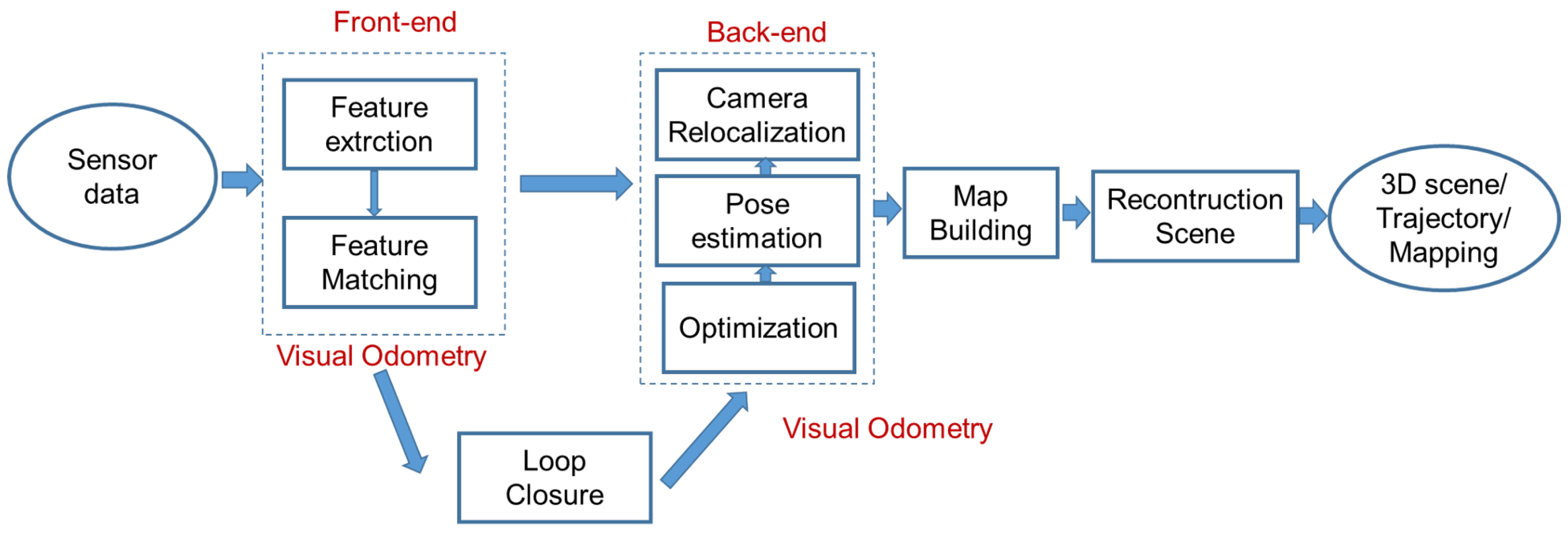
3. Visual SLAM and Visual Odometry Using Deep Learning: Survey

As shown in Figure 2, the paper surveys Visual SLAM and VOE based on the RGB-D images captured from image sensors. In this study, we only surveyed studies conducted based on DL.

3.1. Deep Learning-Based Module for Visual SLAM and Visual Odometry

As in the [29] study, the Visual SLAM model includes the following modules: depth estimation, optical flow, VOE, mapping, and loop closure detection. The study of [7] presents the survey according to the architecture of DL. In contrast in this paper, we present the modules for the architecture of DL networks to build the Visual SLAM system in the following.

3.1.1. Depth Estimation

a. Methods
According to the depth estimation module, Eigen et al. [40] proposed a deep network consisting of two stacks to directly regress depth using the coarse-scale network to estimate the global structure of the scene and using the fine-scale network to refine it using local information. Chen et al. [41] proposed a deep network which is a variation of the hourglass to estimate depth by training a multi-scale deep network and relative depth annotations of the data. The input for pixel-wise depth prediction is a single image. Zhou et al. [42] proposed an end-to-end learning deep network for a single-view depth (scene structure) and pose estimation (camera motion) from the image sequence. To predict single-view depth, the DispNet network architecture was used in an encoder–decoder design. To predict the pose of the camera, the target view was concatenated with all the source views according to the color channel of the input image sequence. Wang et al. [43] proposed a method to improve the method performance of [42] for depth estimation and camera pose by the CNN-based with a simple normalization step, thereby significantly improving the performance of depth estimation. In the proposed approach; the authors applied a Direct Visual Odometry (DVO) [44] pose predictor to predict the output pose based on the input dense depth map, thereby reducing information loss of sequence frames during scene reconstruction. Garg et al. [45] proposed an unsupervised CNN learning method based on auto-encoder architecture to predict single view depth without requiring learning from annotated GT depths. The loss function in this CNN represents the difference between the source image and the inverse-warped target image; it represents the correlation of the prediction error and aligns two different depth maps without using the GT of depth maps. Godard et al. [46] proposed an end-to-end unsupervised DL network to estimate monocular depth with a new information loss function that enforces left–right depth consistency inside the network. The information loss function is capable of combining three error information: smoothness/disparity smoothness loss, reconstruction/appearance matching loss, and left–right disparity consistency terms/left–right disparity consistency loss. The loss function is the sum of the above three error information. Casser et al. [47] proposed an unsupervised DL method based on exploiting 3D geometry structure and semantics to build a model to estimate scene depth and ego-motion. The input of the learning method is a sequence of RGB frames and performs the following calculation steps: object masks, object ego-motion, and individual object motion. The output of the learning model is the image warped according to ego-motion. Bian et al. [48] proposed an unsupervised DL network for estimating depth and motion from two consecutive frames of monocular video. The feature used for the training process is a geometry consistency constraint extracted from a self-discovered mask for dynamic scenes and occlusions to enforce scale consistency, from which the motion of a global scale can be estimated.
Most of the studies presented above only used RGB images as input to the DL network to estimate the depth of the scene, as researched by [47] by moving objects in a frame sequence to estimate scene depth based on how fast objects move between pairs of color image frames. These studies aim to only use RGB images of cheap cameras without paying attention to the depth data of the datasets presented below.
b. Datasets
KITTI Dataset: The KITTI dataset [9,10,11] is the most popular database for evaluating Visual SLAM and VOE models and algorithms. This database includes two versions: the KITTI 2012 dataset [10] and the KITTI 2015 dataset [11]. The KITTI dataset is a computer vision dataset for autonomous driving research. It includes more than 4000 high-resolution images, LIDAR point clouds, and sensor data from a car equipped with various sensors. The dataset provides annotations for object detection, tracking, and segmentation, as well as depth maps and calibration parameters. The KITTI dataset is widely used to train and evaluate DL models for automated driving and robotics. KITTI dataset is collected from two high-resolution camera systems: a Velodyne HDL-64E laser scanner (grayscale and color) and a state-of-the-art OXTS RT 3003 localization system (a combination of devices such as GPS, GLONASS, security IMU, and RTK correction signals). These devices were mounted on a car and collected data over a distance of 39.2 km. The resolution of the image produced is 1240 × 376 pixels. The GT data for evaluating Visual SLAM models and VO include 3D pose annotation data of the scene. The GT data to evaluate object detection models and 3D orientation estimation include accurate 3D bounding boxes for object classes. The 3D object’s point cloud data are marked through manual labeling. In the improved dataset of the KITTI dataset, Menze et al. [11] developed additional data to evaluate the optical flow algorithm. The authors used the 3D CAD model in the Google 3D Warehouse database to build 3D scenes with static elements and insert moving objects.
The NYUDepth dataset was proposed by [49]. The authors used Microsoft (MS) Kinect to collect data from three US cities with 464 different indoor scenes and classified them into 26 scene classes with a total of 1449 RGB-D images/3D scenes. Within the scenes, there are 35,064 distinct objects spread across 894 different classes and labeled manually.
The Make3D dataset was proposed by [50]. This database includes 534 pairs of RGB-D images and color images, with a resolution of 2272 × 1704 pixels, and depth images with a resolution of 55 × 305 pixels. The training data include 400 images, and the testing data include 134 images collected from a 3D scanner. In addition, this database was also supplemented with 588 image pairs from the Internet by someone not part of the data collection project with a size of 800 × 600 pixels.
The Cityscapes dataset was proposed by [51]. This dataset was collected from stereo cameras using 1/3 in CMOS 2 MP sensors (OnSemi AR0331) in 50 different cities of outdoor environments. It has been used to evaluate object detection and classification models, especially DL models. The GT data were prepared with 5000 manually annotated images from 27 cities in a dense pixel-level method. In addition, it is also supplemented with 20,000 raw pixel-level annotated images for evaluating object detection using object boundaries.
The TUM RGB-D SLAM dataset was proposed by [12]. This database used the MS Xbox Kinect sensor to collect RGB-D frame sequences in two environments with sizes of 6 × 6 m2 and 10 × 12 m2, respectively. The first environment is in the office, and the second environment is in a large industrial hall. This database includes 39 RGB-D frame sequences with a size of 640 × 480 pixels and an acquisition rate of 30 Hz, and they are divided into four groups as follows: calibration, testing and debugging, handheld SLAM, and robot SLAM.
The ICL-NUIM dataset was proposed by [13]. This database includes RGB-D sequences collected in the living room and the office room by MS Kinect. It has been used to evaluate VO models, 3D reconstruction, and SLAM algorithms. The GT includes 3D camera trajectories and synthetic trajectories data built on RGB-D images and adds noise from color images and noise from depth images.
c. Evaluation measures
To evaluate depth estimation models, the Root Mean Squared Error ( R M S E ) measure is often used. The R M S E is the square root of the average of the squared errors. The R M S E is the standard deviation of the residuals (prediction error). The residual is a measure of distance from the regression line data points; the R M S E is a measure of how spread out these residuals are. In other words, it tells you how concentrated the data are around the line of best fit. The R M S E includes the R M S E l i n e a r expressed in Formula (1) and R M S E l o g expressed in Formula (2).
R M S E l i n e a r = i = 1 N y i y i * 2 N
R M S E l o g = i = 1 N l o g y i l o g y i * 2 N
where N is the number of data points, y i is the predicted depth map, and y i * is the GT depth map. The R M S E l i n e a r and R M S E l o g have values as small as possible.
d. Results and discussions
The results of evaluating depth estimation on KITTI, NYUDepth, Make3D [50], Cityscapes [51], TUM RGB-D SLAM, and ICL-NUIM datasets with R M S E l i n e a r and R M S E l o g measurements are shown in Table 2. The evaluation results of DRM-SLAM_F [52] on the NYUDepth dataset [49] are the best. The evaluation results of Cowan-GGR [53] on the KITTI dataset are the best. The evaluation results of DVO_CNN [43] on the Make3D dataset [50] are the best. The evaluation results of DRM-SLAM_F [52] on the TUM RGB-D SLAM dataset are the best. The evaluation results of PE_N [54] on the ICL-NUIM dataset are the best. In Table 2, the KITTI dataset was evaluated in most studies, and the Make3D and Cityscapes datasets were evaluated in only a few studies. Table 2 also shows studies on the depth estimation evaluated across multiple datasets, so equal comparisons across studies are difficult to make. Therefore, Table 2 has many empty cells.

3.1.2. Optical Flow Estimation

a. Methods for optical flow estimation
By the optical flow estimation module, [55] proposed and compared two end-to-end CNN architectures for optical flow estimation from a pair of images: FlowNetSimple and FlowNetCorr. It is called FlowNet. FlowNetSimple uses a generic network with two stacked input images to extract motion information for optical flow prediction. The FlowNetCorr creates two identical streams for each image of the input image pair and then combines the two streams to predict the optical flow. Ilg et al. [56] proposed a deep network method to improve the FlowNet of [55] for optical flow estimation called FlowNet 2.0. The proposed method includes three important improvements: The first is concerned with the training data; it was trained on the FlyingChairs dataset and FlyingThings3D dataset to exploit the quality of training data for optical flow estimation.
The second is to develop a stacked architecture to warp with the previously estimated flow. The third addresses small displacements by introducing a subnetwork specializing in small motions. This improved version made the accuracy increase four times and the speed increases more than 17 times. Ranjan et al. [57] proposed an approach by applying the spatial pyramid formula to DL, with the idea of applying a coarse-to-fine approach to calculating and updating the flow at each pyramid level by warping an image of a pair. The number of parameters of this network was reduced by 96% compared to FlowNet by applying the Spatial Pyramid Network, the flow at each pyramid level applied a conv. network to pairs of warped images, and learned convolution filters were applied, like spatio-temporal filters, into the network to improve the FlowNet network.
Sun et al. [58] proposed PWC-Net, which is a combination of pyramidal processing, warping, and a cost volume for optical flow estimation. It is an improved model from Spatial Pyramid Network [57] and FlowNet 2.0 [56].
Table 2. Depth estimation results based on DL.
Authors/YearsDataset/
Measu./
Methods
NYUDepthKITTI
2012
Dataset
Make3D
Dataset
Cityscapes
Dataset
TUM RGB-D
SLAM
Dataset
ICL-NUIM
Dataset
RMSE
Linear
RMSE
Log
RMSE
Linear
RMSE
Log
RMSE
Linear
RMSE
Log
RMSE
Linear
RMSE
Log
RMSE
Linear
RMSE
Log
RMSE
Linear
RMSE
Log
[40]/2014Multi-Scale
DN
2.190.2855.2460.2488.3250.409------
[59]/2015CRF_
CNN
0.82-----------
[60]/2015Ordinal
Relationships
DN
1.20.42----------
[61]/2015HCRF_CNN0.750.26----------
[62]/2015SGD_DN0.640.23------1.410.370.830.43
[63]/2016CRF_
CNN_N
0.730.33------0.860.290.810.41
[41]/2016Pixel-wise_
ranking DN
0.240.38----------
[64]/2016Deeper FCRN0.510.22------1.070.390.540.28
[45]/2016Unsupervised
CNN
--5.1040.2739.6350.444------
[46]/2017Unsupervised
CNN_D
--6.1250.2178.860.14214.4450.542----
[42]/2017SfMLearner--4.9750.25810.470.478------
[54]/2017PE_S0.520.21------0.690.250.320.18
[54]/2017PE_N0.450.17------0.650.240.220.12
[65]/2018StD0.480.17------0.70.270.360.18
[66]/2018RSS0.450.18------0.650.240.330.19
[67]/2018Pre-trained
KITTI +
Cityscapes
--6.6410.248--------
[43]/2018DVO_CNN--5.5830.2288.090.204------
[67]/2018Pre-trained
KITTI
--6.50.27--------
[68]/2018Pre-trained
KITTI
--6.220.25--------
[69]/2018Geonet-VGG
pre-trained KITTI
--6.090.247--------
[69]/2018Geonet-Resnet
Pre-trained KITTI
--5.8570.233--------
[70]/2018DF-Net
Pre-trained KITTI
--5.5070.223--------
[68]/2018Pre-trained
KITTI + Cityscapes
--5.9120.243--------
[69]/2018Geonet-Resnet
Pre-trained KITTI +
Cityscapes
--5.7370.232--------
[70]/2018DF-Net
Pre-trained
KITTI + Cityscapes
--5.2150.213--------
[65]/2018StD- RGB0.510.21----------
[66]/2018RSS-RGB0.730.19----------
[71]/2019Pre-trained
KITTI + Cityscapes
--5.1990.213--------
[71]/2019Pre-trained
KITTI
--5.3260.217--------
[48]/2019Pre-trained
KITTI
--5.4390.217--------
[48]/2019Pre-trained
KITTI + Cityscapes
--5.2340.208--------
[47]/2019Struct2depth--5.2910.215--------
[72]/2019Monodepth2--4.7010.19--------
[52]/2020DRM-
SLAM_F
0.420.16------0.620.230.30.13
[73]/2020Packnet-sfm--4.6010.189--------
[52]/2020DRM-
SLAM_C
0.50.19------0.70.280.360.18
[74]/2020EPC++--5.350.216--------
[75]/2021Faster
R-CNN
AVN
--4.7720.191--------
[53]/2022Cowan-GGR--3.9230.188--------
[53]/2022Cowan--4.9160.212--------
The input of PWC-Net is still a pair of images, and the CNN features of the second image are calculated based on the current optical flow of the first image. The warped features of the image pair are used to construct a cost volume. PWCNet’s calculation time is only 1/17 of FlowNet 2.0.
Teed et al. [76] proposed the RAFT network for optical flow estimation. RAFT includes (1) the per-pixel features of image pairs extracted using a feature encoder module, 4D correlation volume built and synthesized from all pairs of feature vectors using a feature encoder module, and (3) an update module iterated on recurrently optical flow by lookups on the correlation volumes.
Ren et al. [77] proposed an unsupervised DL network called Dense Spatial Transform Flow (DSTFlow) that estimates optical flow based on input frame pairs. This is an end-to-end learning consists of three components: a localization layer, sampling layer, and interpolation layer. Backpropagation is used to train the parameters in all three layers.
Zhu et al. [78] proposed an unsupervised CNN framework to estimate optical flow based on proxy GT data. These data are responsible for guided optical flow learning and consist of two stages: The first is a GT flow proxy created based on classical approaches, and the second is the process of fine-tuning the model using image-minimizing reconstruction loss.
Wang et al., [79] proposed an end-to-end deep neural network to estimate optical flow based on learning large motions using occlusion models clearly and a new warping. The main flow of this method is to use two copies of FlowNetS to share parameters and estimate forward and backward optical flow. Janai et al. [80] proposed a new unsupervised learning framework for optical flow estimation based on multiple frames by exploiting the temporal relationship between frames and occlusions jointly. The flow fields and occlusion map are estimated based on evaluating the loss function of the warped images.
Zhong et al. [81] proposed an unsupervised learning network for optical flow estimation called Deep Epipolar Flow. It uses soft Epipolar constraints on the low level and subspace of the scene when not in motion. The unsupervised training process is optimized based on image-based losses and Epipolar constraint losses. Liao et al. [82] proposed a method to estimate optical flow based on a combination of utilizing intrinsic image decomposition and recomposition based on Retinex theory on two consecutive frames of outdoor UAV videos and an edge refinement scheme based on weighted neighborhood filtering.
Yan et al. [83] proposed a semi-supervised DL network to estimate optical flow. The proposed network is based on direct estimation from real data without using GT data. Foggy images and optical flow modules are estimated from clean images based on domain transformation. These two data sources interact together, wherein the optical flow module and the flow map that produces the flow map must be the same to generate the same error.
Dai et al. [84] proposed a self-supervised learning framework for depth and object motion estimation, in which the motion of individual objects is predicted based on rotation and translation of six degrees of freedom. The proposed network consists of two subnets: The objMotion-net and the Depth-net. The pose network is used to design ObjMotion-net, and Depth-net is designed based on the encoder and the decoder structure, with the basic structure being ResNet50.
Ranjan et al. [71] proposed an unsupervised training framework of multiple specialized neural networks called Competitive Collaboration to perform depth estimation, camera motion estimation, optical flow, and segmentation. This general framework solves the problem by dividing the scene into moving objects and static background, camera motion, depth of static scene structure, and optical flow of moving objects.
b. Datasets of optical flow estimation
MPI Sintel dataset [85]: To evaluate optical flow estimation models, [85] have published the MPI Sintel dataset. This database was created from 3D animations built from Sintel open-source code. Based on the cartoon, the camera’s parameters, moving objects, and graphics are all calculated using vectors. The original data for optical flow estimation are also provided in the form of vectors. This database includes 35 clips, with 23 clips (1064 frames) used for training and 12 clips (564 frames) used for model testing. In it, the process of creating the database was carried out in three different ways: The first was “Albedo”; these data used the simplest pass of constant color with almost no lighting effect. The second was “Clean”; the data using this pass added complexity by introducing various types of lighting that make smooth gloss surfaces, self-shadowing, darkening in cavities, and darkening where the object is close to the surface. The third was “Final”; these data were similar to the released film and added some effects such as atmospheric effects, depth of field blur, motion blur, and color correction.
Middlebury dataset [86]: Unlike other datasets, this dataset has a very small number of frames, consisting of only eight frames, and the original data were determined in the middle pair. The authors not only collected color images but also created grayscale images. The data were divided into 12 sequences for training with original data and 12 sequences for testing.
Flying Chairs dataset [55]: The GT data are the model of the chair. These data include 22,872 image pairs and corresponding flow fields. Among them, 964 images were collected from Flick with the environments ‘city’, ‘landscape’, and ‘mountain’, with a resolution of 1024 × 768 . From this original image, the authors cropped images with dimensions 512 × 384 in four quadrants. Chair objects were added to the background, resulting in 809 chair types with 62 views per chair.
Foggy dataset [83]: This is a synthetic dataset built by combining the defogging method with the original FlowNet2 [56], PWCNet [58], and CC [71] datasets. The defogging method was proposed by [87]. The generated data include 2346 real fog image pairs used for training, and the GT includes 100 real fog image pairs that were annotated manually.
c. Evaluation measure of optical flow estimation
To evaluate the results of the optical flow estimation, methods often use the End-Point Error ( E P E ) losses measure between the predicted optical flow ( V e ) and GT ( V g t ), as computed in the Formula (3). The unit of measurement is pixels. Based on the evaluation measure, if the E P E is small, the optical flow estimation model is better.
E P E = V e V g t
d. Results and discussions of optical flow estimation
The results of optical flow estimation are shown in Table 3. The results were evaluated on seven datasets when evaluated on the Sintel Clean dataset [85], and the best results were with the method of [82] (FlowNet2-IAER). On the Sintel Final dataset [85], the best results were from the method of [82] (FlowNet2-IAER). On the KITTI 2012 dataset, the best result was that of the method of [81] (sub-test-ft). On the KITTI 2015 dataset [11], the best results were from the method of [77]. On the Middlebury dataset [86], the best results were from the method of [88]. On the Flying Chairs dataset [55], the best result was that of the method of [78]. Finally, on the Foggy dataset [83], the best result was that of the method of [83]. The results show that more recent studies tend to have lower error rates. However, studies often focus on evaluating a few datasets—Sintel Clean, Sintel Final, KITTI 2012, and KITTI 2015—so there are many empty results on the remaining datasets.

3.1.3. Keypoint Detection and Feature Matching

a. Methods for keypoint detection and feature matching
Regarding the keypoint detection and feature matching categories, Hart et al. [89] proposed a method to detect keypoints and feature matching by finding a description prediction model before performing matching. The points were well-located and repeatable, which also reduced the number of points of interest and the time needed to consider points for the matching process. Verdie et al. [90] proposed a method that allows detecting keypoints and feature matching based on a training method to identify potentially stable points on the training image by creating a regression set of points of a score map whose values are local maxima at these locations. Shen et al. [91] proposed an end-to-end matching network based on improving LF-Net; the proposed method proposes a scale space structure with the corresponding map for keypoint detection. Second, the training patch is selected based on the general loss function and neighbor mask.
Recently, Liu et al. [92] tested SuperPoint and SuperGlue into the OpenVINS framework for keypoint detection and feature matching. The results showed that using SuperPoint and SuperGlue in the VO system was not optimal when experimenting on the EuRoC dataset. Wang et al. [93] proposed OFPoint, which is a self-supervised detector based on transfer learning to perform optical flow tracking in a VOE system. The fine-tuning of SiLK as the pre-trained network is used to avoid relearning high-dimensional point features. Multi-scale attention mechanism that captures salient point features at different scales is used. Burkhardt et al. [94] proposed a data-driven SuperEvent method to predict stable keypoints. Due to the lack of ground truth keypoint labels, the authors proposed A to leverage existing frame-based keypoint detectors on available event-aligned and synchronized grayscale frames for self-supervision. Dusmanu et al. [95] proposed D2-Net for determining a dense feature descriptor and a feature detector between two frames. D2-Net includes a two-stage detect-then-describe function for correspondings to different variants and uses a single CNN to extracts dense features. Li et al. [96] proposed DXSLAM for feature extraction in the loop closure, global optimization, and relocalization steps of a Visual SLAM model. This feature extractor is integrated in Intel OpenVINO toolkit.
b. Datasets for keypoint detection and feature matching evaluation
To evaluate the results of keypoint detection and feature matching, Verdie et al. [90] used the following datasets.
Webcam dataset [90]: This is a dataset consisting of six scenes, of which five scenes (St. Louis, Mexico, Chamonix, Courbevoie, and Frankfurt) were selected from the AMOS [97] dataset, and the Panorama scene was collected from the roof with a 360 degrees view.
Oxford dataset [98]: This is a small dataset consisting of eight scenes (viewpoint changes (1) and (2); scale changes (3) and (4); image blur (5) and (6); JPEG compression (7); and illumination (8)). On the data, there are two types of changes: scene type and image condition. In a scene, there are two types of variable regions: one (a) containing uniform regions with distinctive edge boundaries and (b) the other containing repeating motifs in different forms.
EF dataset [99]: This is a small dataset consisting of five sequences of 38 images which contain drastic illumination and background clutter changes.
HPatches(HP) dataset [100]: This is a database consisting of 116 sequences built from six images with known patterns in nature and man-made scenes; it is divided into two parts: (1) HP-viewpoint includes 59 sequences with significant viewpoint changes; (2) HP-illumination includes 57 sequences with significant illumination changes. The data of these two sets are divided into 90% for training and validation and 10% for testing. During the training process, the data are standardized to a size of 320 × 240 .
c. Evaluation measure of keypoint detection and feature matching evaluation
To evaluate the results of the keypoint detection and feature matching process, studies often use the measure of repeatability, of which there are two evaluation cases: The first is to evaluate the repeatability in the case of taking the ratio; the main score is 2% of the score on the image (2%). The second is that a keypoint cannot be used more than once when evaluating repeatability (stand.). Based on the results of these two measurements, the higher result is the better [90]. Another measure, average match score (AMS), is also evaluated for keypoint detection and feature matching [100].
d. Results of keypoint detection and feature matching evaluation
The keypoint detection and feature matching results based on DL are shown in Table 4. In addition, the authors also compared some traditional methods such as Fast [101], SFOP [102], SIFER [103], SIFT [104], SURF [105], WADE [106], and EdgeFoci [99]. When comparing measures (2%) and (stand.), TILDE [90] had the best results when compared to measure AMS, and RF-Net had the best results. However, the results were evaluated on multiple databases and with different measures, so many cells in Table 4 are empty.
Table 3. The optical flow estimation results based on DL.
Datasets/
Authors/
Years
Sintel
Clean
Dataset
[85]
Sintel
Final
Dataset
[85]
KITTI
2012 [9]
KITTI
2015
Dataset [11]
Middlebury
Dataset
[86]
Flying
Chairs
Dataset
[55]
Foggy
Dataset [83]
Train/Test
( EPE )
Train/Test
( EPE )
Train/Test
( EPE )
Train/Test
( EPE )
Train/Test
( EPE )
Train/Test
( EPE )
Train/Test
( EPE )
[55]/20153.20/6.084.83/7.886.07/7.6-3.81/4.52--
[56]/20171.45/4.162.01/5.741.28/1.82.30/-0.35/0.52--
[57]/20173.17/6.644.32/8.368.25/10.1 0.33/0.58-/3.07-
[77]/20174.17/5.305.45/6.163.29/4.00.36/0.39---
[78]/2017-/3.01-/7.96-/9.5---/3.01-
[58]/20182.02/4.392.08/5.041.45/1.72.16/----
[79]/20184.03/7.955.95/9.153.55/4.28.88/---/3.76-
[80]
(Hard)
/2018
5.38/8.356.01/9.38-8.8/----
[80]
(Hard-ft)
/2018
6.05/-7.09/--7.45/----
[80]
(None-ft)
/2018
4.74/-5.84/--3.24/----
[80]
(Soft-ft)
/2018
3.89/7.235.52/8.81-3.22/----
[81]
(baseline)
/2019
6.72/-7.31/-3.23/-4.21/----
[81]
(gtF)
/2019
6.15/-6.71/-2.61/-2.89/----
[81]
(F)
/2019
6.21/-6.73/-2.56/-3.09/----
[81]
(low-rank)
/2019
6.39/-6.96/-2.63/-3.03/----
[81]
(sub)
/2019
6.15/-6.83/-2.62/-2.98/----
[81]
(sub-test-ft)
/2019
3.94/6.845.08/8.332.61/1.12.56/----
[81]
(sub-train-ft)
/2019
3.54/7.04.99/8.512.51/1.32.46/----
[88]/2019-/3.748-/5.81-/3.5--/0.33-/2.45-
[83]
/2020
---/1.6----/4.32
[82]
(PWC-Net-ft)
/2021
2.02/4.392.08/5.041.45/1.7----/6.10
[82]
(FlowNet2-ft)
/2021
1.45/4.162.01/5.741.28/1.8----/4.74
[82]
(FlowNet2-IA)
/2021
1.52/4.115.51/1.41.4/1.8----/4.72
[82]
(FlowNet2-IAER)
/2021
1.46/4.062.13/1.371.37/1.8----/5.19
[93]
(OFPoint)
/2025
-/--/--/0.065----/-
Table 4. The keypoint detection and feature matching results based on DL.
Authors/YearsDatasets/
Measu./
Methods
Webcam
Dataset
Oxford
Dataset
EFHP-
Viewpoint
Dataset
HP-
Illumination
Dataset
2%Stand.2%Stand.2%Average
Match
Score
Average
Match
Score
Average
Match
Score
[104]/2004SIFT20.746.543.632.2230.2960.490.494
[101]/2006Fast26.453.847.93928---
[105]/2006SURF29.956.957.643.628.70.2350.4930.481
[102]/2009SFOP22.951.339.342.221.2---
[99]/2011EdgeFoci3054.947.546.231---
[103]/2013SIFER25.745.140.127.417.6---
[106]/2013WADE27.544.35125.628.6---
[90]/2015TILDE-GB33.354.532.843.116.2---
[90]/2015TILDE-CNN36.851.849.343.227.6---
[90]/2015TILDE-P2440.758.759.146.333---
[90]/2015TILDE-P48.358.155.945.131.6---
[107]/2017L2-Net+DoG-----0.1890.4030.394
[107]/2017L2-Net+SURF-----0.3070.6270.629
[107]/2017L2-Net+FAST-----0.2290.5710.431
[107]/2017L2-Net+ORB-----0.2980.7050.673
[107]/2017L2-Net+Zhang et al.-----0.2350.6850.425
[108]/2017Hard-Net+DoG-----0.2060.4360.468
[108]/2017Hard-Net+SURF-----0.3340.650.668
[108]/2017Hard-Net+FAST-----0.290.6170.63
[108]/2017Hard-Net+ORB-----0.2380.6160.632
[108]/2017Hard-Net+Zhang et al.-----0.2730.6710.557
[109]/2018LF-Net-----0.2510.6170.566
[91]/2019RF-Net-----0.4530.7830.808
[93]/2025OFPoint------0.6170.678

3.1.4. DL Modules Add to the Visual SLAM Algorithm

a. Feature extraction module DL
Qin et al. [110] proposed a keypoint extraction network used to resemble the Oriented FAST and Rotated BRIEF (ORB)-SLAM2 module in VOE. Therefore, SP-Flow is used to replace ORB-SLAM2 in VOE construction. This network is called SP-Flow. It is a combination of a self-supervised framework and the Lucas–Kanade method. The self-supervised framework of SP-Flow includes three stages: keypoint pre-training, keypoint self-labeling, and joint training. In the Visual SLAM model, whether feature extraction is effective often depends on the feature point extraction for a single image and its feature point matching accuracy between two successive frames. SP-Flow has tried to simplify the feature extraction process but still ensures accuracy. The architecture of SP-Flow includes six conventional convolution layers.
Bruno et al. [111] proposed a module based on the Learned Invariant Feature Transform (LIFT) in the traditional ORB-SLAM Visual SLAM construction method. This module is responsible for extracting features from images for ORB-SLAM. The architecture of LIFT is based on a CNN consisting of three modules: detector, orientation estimator, and descriptor. It is a very important module in ORB-SLAM, and LIFT has been pre-trained on many VOE datasets.
Studies based on this approach have performed evaluations on databases such as the TUM RGB-D SLAM dataset [12], the KITTI 2012 dataset [9], and the Euroc dataset [36]. The TUM RGB-D SLAM [12] and the KITTI 2012 [9] datasets have been presented above.
The Euroc dataset [36] was collected onboard a Micro Aerial Vehicle (MAV) based on the stereo camera and synchronized IMU measurements. This dataset has been used to evaluate the visual–inertial SLAM and 3D reconstruction capabilities. The data include 11 stereo sequences collected from slow flights under good visual conditions to dynamic flights with motion blur and poor illumination with two types of data—images collected from industrial scenarios and images collected from inside a Vicon motion capture system—with obstacles placed over the scene.
To evaluate the results of the Visual SLAM algorithm using the DL module for feature extraction, the methods use several evaluation metrics as follows: (1) The absolute trajectory error ( A T E ) [12] is the distance error between the GT A T ^ i and the estimated motion A T i trajectory. The A T E is calculated according to Formula (4).
A T E = 1 N i N | | T A T i A T ^ i | | 2
where N is the number of frames in the video used to estimate VOE.
(2) t r e l and r r e l measurements: t r e l is the average transnational R M S E drift (%) on a length of 100–800 m. r r e l is the average rotational R M S E drift (°/100 m) on a length of 100–800 m.
The results of Visual SLAM when using the feature extraction module using DL are shown in Table 5. The results are based on the A T E , t r e l , and r r e l measurements, wherein the smaller they are, the better. The results are evaluated on three databases with three types of measures, and each method only evaluates one dataset and one type of measure. Therefore, Table 5 still has many empty results. Table 5 also shows that the error results on TUM RGB-D SLAM and Euroc datasets are very low (0.03–0.5 m). The results show that RTG-SLAM [112] has the best result, with an error of 0.0106 m = 1.06 cm; SplaTAM [113] also has a very small error of 0.0339 m = 3.39 cm. These are very good results that can be applied to building practical applications in building Visual SLAM for robots and visually impaired people to find their way in indoor environments. The VO time and map construction time of SplaTAM [113] were 0.19 s/frame, and 0.33 s/frame, respectively, when performing calculations on a GPU RTX 3080 Ti, which are close to the real calculation time and can meet the requirements of practical applications. The results on the KITTI 2012 dataset are very large (8–11 m). This proves that choosing a standard dataset for evaluating the feature extraction problem also has many challenges.
b. Semantic segmentation module DL
Sun et al. [114] proposed MR-SLAM to improve the results of the RGB-D SLAM. The main idea of this approach is to use the RGB-D data-based motion removal approach and integrate it into the front end of the RGB-D SLAM. The input data of MR-SLAM is RGB-D data; first, the ego-motion compensated image differencing is used to detect moving objects, then a particle filter is used to detect motion, and finally, a Maximum-a-posterior (MAP) estimator is applied on vector quantized depth images to construct the foreground.
Kaneko et al. [115] proposed a framework to improve the efficiency of Visual SLAM by using the results of mask-based semantic segmentation to identify feature points extraction regions (detect and segment several objects on the image). The object mask problem is implemented using DeepLab v2 [116]. This helps reduce the number of incorrect matches between correspondences when using RANSAC. The authors applied ORB-SLAM to the framework to build Visual SLAM.
Yu et al. [117] proposed DS-SLAM to improve localization efficiency in dynamic environments when performing pose estimation. DS-SLAM has five threads running in parallel: tracking, semantic segmentation, local mapping, loop closing, and dense semantic map creation. In particular, the local mapping thread and loop closing thread are implemented similarly to ORB-SLAM2. DS-SLAM uses the raw RGB image is utilized to semantic segmentation and moving consistency check simultaneously via SegNet and RANSAC, respectively. Finally, the global octo-tree map is built based on the combination of the local point clouds created from the keyframes’ transform matrix and the depth images.
Table 5. Results of Visual SLAM when using the feature extraction module using DL.
Authors/YearsDataset/
Measu./
Methods
TUM RGB-D
SLAM
Dataset
KITTI 2012
Dataset
Euroc
Dataset
ATE (m) t rel (%) r rel (deg/100 m) ATE (m) ATE (m)
[118]/2017ORB-SLAM2
(stereo)
-0.7270.22--
[119]/2019GCN-SLAM0.05----
[110]/2020SP-Flow
SLAM
0.03----
[110]/2020Stereo
LSD-SLAM
-0.9420.272--
[110]/2020SP-Flow
SLAM(stereo)
-0.760.19--
[111]/2020LIFT-SLAM---9.190.573
[111]/2021LIFT-SLAM
(fine-tune KITI)
---11.330.08
[111]/2021LIFT-SLAM
(fine-tune Euroc)
---8.940.07
[111]/2021Adaptive
LIFT-SLAM
---8.560.04
[111]/2021Adaptive
LIFT-SLAM
(fine-tune KITI)
---11.240.28
[111]/2021Adaptive
LIFT-SLAM
(fine-tune Euroc)
---11.30.048
[120]/2023Point-SLAM0.0892----
[121]/2023ESLAM0.0211----
[122]/2023Co-SLAM0.0274----
[113]/2024SplaTAM0.0339----
[112]/2024RTG-SLAM0.0106----
[123]/2024SG-Init+
DROID(L)
--9.07-
[123]/2024SG-Init+
DROID (O)
--9.39-
[123]/2024SG-Init+
DROID (N/A)
--14.92-
[124]/2024LGU-VO -- 0.139
[124]/2024LGU-SLAM0.031-- 0.018
[124]/2024LGU (w/o SSL) -- 0.142
[124]/2024LGU (w/o SM) -- 0.146
Bescos et al. [125] proposed DynaSLAM based on ORB-SLAM2. DynaSLAM’s input data are in dynamic scenarios for monocular, stereo, and RGB-D images. DynaSLAM can detect moving objects using multi-view geometry, DL, or both types of models. The pixel-wise semantic segmentation of dynamic objects with stereo and monocular input data is performed using Mask R-CNN, with RGB-D data using the multi-view geometry method for rendering. The mapping and tracking steps are performed based on ORB-SLAM2.
Zhong et al. [126] proposed Detect-SLAM based on integrating ORB-SLAM2, which involves an object detection module using a Single-Shot Multi-box Object Detector (SSD). Detect-SLAM also includes three parallel streams: tracking, local mapping, and loop closing. However, there are the following new points: First, Detect-SLAM only cares about moving objects. The second is that the static objects are reconstructed on keyframes according to the point cloud data and the object map is also constructed. The third is to improve object detection results using a SLAM-enhanced detector.
Tian et al. [127] proposed a novel framework for the Visual SLAM system based on the combination of Faster RCNN for object detection, semantic segmentation in 3D space, and the estimation results from the SLAM system. The input data of the framework are obtained as an RGB-D image. First, the local target map is built using CNN to detect the 2D object proposals. Then, the dynamic global target map is updated based on the local target map obtained by CNNs. Finally, the detection result of the current frame is obtained by projecting the global target map into 2D space. Cheng et al. [128] proposed OFB-SLAM to improve the results of the Visual SLAM system in the case of a dynamic environment. OFB-SLAM uses optical flow in a feature-based monocular SLAM system to remove dynamic feature points on the input frame. It includes two modules: ego-motion estimation and dynamic feature points detection. The ego-motion estimation module extracts the feature points from the current frame and the previous frame; to find the corresponding feature pair between the two frames, RANSAC is used. Optical flow is used to detect object motion. OFB-SLAM is integrated into ORB-SLAM and implements the next steps of the Visual SLAM system.
Shao et al. [129] proposed a method to filter outliers of RANSAC-based F-matrix calculations using faster R-CNN. Therein, the inliers are trained using semantic patches tailored which can provide semantic labels of image regions. From there, low-quality feature areas are effectively reduced. The proposed method is added to the ORB-SLAM system. Xua et al. [130] proposed Deep SAFT to improve feature-based vSLAM’s applicability in more challenging environmental conditions. Deep SAFT is an online learning scene adaptation feature transform that is capable of self-adapting to recently observed scenes by taking advantage of the advantages of CNN. The authors used Deep SAFT to replace ORB-SLAM2 in the Visual SLAM system.
Liu et al. [131] proposed the Edge-Feature Razor (EF-Razor) method. EF-Razor first uses semantic information offered by the real-time object detection method YOLOv3 to distinguish edge features. To effectively filter unstable features onto the SLAM system, EF-Razor was used. The authors integrated EF-Razor into ORB-SLAM2. Rusli et al. [132] proposed a semantic SLAM using method objects and walls as a model of an environment, called RoomSLAM. RoomSLAM includes two modules running in parallel: front-end and back-end. The front-end performs object detection and wall detection using YOLOv3 on RGB images, and depth images are converted to point cloud data to determine the location of objects and walls in the 3D space of the real world. They are seen as landmarks of the environment, and the walls are used to construct rooms in the scene. The back-end is responsible for estimating the state through the optimization graph. In RoomSLAM, a second component that is also very important is the room. RoomSLAM also looks for similarities between rooms to detect loop closures. Jin et al. [133] proposed an Unsupervised Semantic Segmentation SLAM framework, called USS-SLAM, to improve robot positioning accuracy when moving. This framework is integrated into ORB-SLAM2. To do this, USS-SLAM filters out dynamic features using a semantic segmentation model learned from the DeepLab V2 unsupervised learning network, whose backbone is ResNet. This learning method can be trained by the adversarial transfer learning method in multi-level feature spaces. The next steps of the Visual SLAM system are based on ORB-SLAM2.
Zhao et al. [134] proposed a semantic visual–inertial SLAM system for dynamic environments based on VINS-Mono [135] with three streams: RGB-image manager, semantic segmentation manager, and feature point processing. In particular, RGB-image manager and semantic segmentation manager use the RGB-images and the semantic segmentation result. The feature point processing flow uses the optical flow to track feature points on the RGB frames. The result of this research is that it is possible to perform real-time trajectory estimation by utilizing the pixel-wise results of semantic segmentation.
Cheng et al. [136] proposed DM-SLAM based on feature-based methods to improve the results of the location accuracy in dynamic environments. DM-SLAM is combined from an instance segmentation network with optical flow information. DM-SLAM includes four modules: semantic segmentation, ego-motion estimation, dynamic point detection, and a feature-based SLAM framework. The semantic segmentation module uses Mask R-CNN for object segment segmentation, followed by moving points being detected and removed in ego-motion estimation. The dynamic feature points are extracted from the dynamic point region detected in the previous step, and finally, the feature-based SLAM framework module uses ORB-SLAM2.
Liu et al. [137] proposed RDS-SLAM to improve the results of building Visual SLAM systems in real-world dynamic environments. RDS-SLAM proposes a semantic segmentation thread that does not have to wait for results from any module, and the tracking thread also does not have to wait for results from the segmentation module. This method helps to effectively perform semantic segmentation results for dynamic object detection and eliminate outliers. The next implementation of RDS-SLAM is based on ORB-SLAM3.
Su et al. [138] proposed a real-time visual SLAM algorithm based on deep learning based on ORB-SLAM2. To extract semantic information in images, a parallel semantic thread is built. To remove dynamic features in the image, the authors used an optimized optical flow mask module. Dynamic objects in images are detected using YOLOv5s built into the semantic thread. To improve the system results in the tracking module, a method of optimizing the homograph matrix is used.
To evaluate the DL module for semantic segmentation added to the Visual SLAM system, the below studies evaluated the following datasets. CARLA [139] was used to study the results of three approaches to autonomous driving: a classic modular pipeline, an end-to-end model trained via imitation learning, and an end-to-end model trained via reinforcement learning. CARLA can provide automated digital environments such as urban layouts, buildings, and vehicles. This can support the development, training, and validation of urban automated driving systems.
ObjectFusion dataset I, ObjectFusion dataset II, ObjectFusion dataset III, and ObjectFusion dataset VI [127] were collected from the Asus Xtion Pro RGB-D sensor and in indoor environments. Trajectories were chosen to build data with many prominent objects as keyframes both locally and globally. ObjectFusion dataset I involves an object in each frame of the scene; the data are a frame sequence consisting of 1801 frames. ObjectFusion dataset II involves multiple objects in each frame of the scene such as chairs, dogs, pot plants, and so on; the data were collected in full lighting conditions and consist of a frame sequence consisting of 1625 frames. ObjectFusion dataset III was collected in a more challenging context; data were collected in a scene with many objects that are occluded in many frames. ObjectFusion dataset VI is similar to ObjectFusion dataset III, and the data were captured in a scene with many objects and moving obstacles.
The ICL-NUIM dataset [13] is an RGB-D benchmarking used to evaluate system VOE and visual SLAM algorithms. Image data compiled from camera trajectories in raytraced 3D models in POVRay with two scenes in the living room and office provide some GT data. Living room GT data include 3D surface GTs, together with the depth maps, camera poses, and camera trajectory, in addition to original data for 3D reconstruction evaluation.
The ADVIO dataset [38] was collected from an iPhone, a Google Pixel Android phone, and a Google Tango device in different indoor and outdoor scenes with 23 sequence frames (7 sequences collected from office indoor scenes, 12 sequences collected from urban indoor scenes, 2 sequences collected from urban outdoor scenes, and 2 sequences collected from suburban outdoor scenes). The GT data include GT trajectory information based on the camera pose GT calculated from the IMU data of the iPhone.
To evaluate the DL module for semantic segmentation added to the Visual SLAM system, the studies evaluated the following measurements.
The Mean Tracking Rate ( M T R ) [115] is the tracking success rate in 50 trials when successful tracking is performed on 80% of the 1000 frames of the sequence, computed based on Formula (5).
M T R = 1 m i = 1 m = 50 ( T r a c k i n g R a t e i )
where T r a c k i n g R a t e i is the “Tracking Rate” (%) at time i t h , and m is the number of times the “Tracking Rate” is performed.
The Mean Trajectory Error ( M T E ) [115] is an estimate of the camera’s position relative to the defined GT, which is the error distance for each time step and the average value of a sequence as “Trajectory Error (m)”. Here, it only calculates the M T E for “Success Tracking” i.e., if the “Tracking Rate” exceeds 80%, the M T E is computed based on Formula (6).
M T E = 1 m i = 1 m ( 1 n i | | X t Y i t | | 2 )
where i = 1 , 2 , , 50 is the number of “Successful Tracking” trials. X t is the 3D position of the GT trajectory, and Y i t is the 3D position of the estimated trajectory over the entire time series ( t = 1 , , n i ) ; n i is the length of the time series for performing the VOE.
The A T E is presented in the Formula (4).
The Intersection over Union ( I O U ) is a measure to evaluate the results of detecting objects in the scene during the process of building the Visual SLAM system, and the I O U is calculated according to Formula (7).
I O U = B B g B B r B B g B B r
where B B g is the bounding box GT of the object, and B B r is the bounding box prediction of the object.
The pixel accuracy ( P A ) is calculated according to Formula (8).
P A = i n i i i t i
The mean precision ( M P ) is calculated according to Formula (9).
M P = 1 n c l i n i i j n j i
where n i j is the number of pixels which classified as j, while the true value is i. n c l is the total classes. t i is the number of pixels that belong to class i, with t i = j n i j .
Another measure used is the absolute translation error R M S E (Tabs) [130], which is the distance between the estimated trajectory and the GT trajectory.
Another type of measure used is the absolute translation (trans.) error R M S E (Tabs) [130], which is the distance between the estimated trajectory and the GT trajectory. The calculation of R M S E (Tabs) was performed in the study of [12]. In [134]’s study, measurements such as R M S E , mean error, and Absolute Pose Error ( A P E ) were used. These measures were also defined in [140].
The results of Visual SLAM when using the DL semantic segmentation module are presented in Table 6.
Table 6. Results of Visual SLAM when using the DL semantic segmentation module.
Authors/YearMethods/
Datasets/
Matrix
CARLATUM
RGB-D
SLAM
Dataset
Object
Fusion
Dataset
I
Object
Fusion
Dataset
II
Object
Fusion
Dataset
III
Object
Fusion
Dataset
IV
ICL-
NUIM
Dataset
ADVIO
Dataset
MTR
(%)/
MTE
(m)
ATE Mean
IOU /
Mean
PA /
MP
Mean
IOU /
Mean
PA /
MP
Mean
IOU /
Mean
PA /
MP
Mean
IOU /
Mean
PA /
MP
RMSE
(Tabs)
RMSE Mean
Error
APE
for
Trans.
[114]/2017MR-SLAM-0.085--------
[115]/2018Mask-SLAM58.2/
13.7
---------
[117]/2018DS-SLAM-0.103--------
[135]/2018VINS-Mono-------5.0374.711.68
[125]/2018DynaSLAM-0.019--------
[126]/2018Detect-SLAM-0.113--------
[127]/2019ObjectFusion-
FCN-VOC8s
--0.52/
0.62/
0.729
0.5169/
0.5966/
0.7103
0.5775/
0.6559/
0.6708
0.3529/
0.4168/
0.7361
----
[127]/2019ObjectFusion-
CRF-RNN
--0.59/
0.63/
0.938
0.4769/
0.4899/
0.5633
0.5618/
0.6058/
0.4115
0.273/
0.2989/
0.5955
----
[127]/2019ObjectFusion-
Mask-RCNN
--0.59/
0.64/
0.895
0.4855/
0.5021/
0.7125
0.4946/
0.5397/
0.4489
0.3433/
0.3938/
0.716
----
[127]/2019ObjectFusion-
Deeplabv3+
--0.58/
0.63/
0.856
0.4849/
0.4927/
0.719
0.4869/
0.537/
0.4458
0.3484/
0.3952/
0.7351
----
[127]/2019ObjectFusion-
SORS
(GLOBAL)
--0.71/
0.726/
0.954
0.5889/
0.6438/
0.7989
0.6063/
0.6764/
0.872
0.4012/
0.4261/
0.7806
----
[127]/2019ObjectFusion-
SORS
(ACTIVATE)
--0.702/
0.724/
0.936
0.5301/
0.5765/
0.8626
0.5528/
0.6106/
0.902
0.3728/
0.3878/
0.7873
----
[128]/2019OFB-SLAM-0.082--------
[129]/2020Semantic
Filter_
RANSAC_
Faster
R-CNN
-0.19--------
[130]/2020Offline
Deep SAFT
-0.0179----0.057---
[130]/2020Continuous
Deep SAFT
-0.168----0.043---
[130]/2020Discrete
Deep SAFT
-0.0235----0.065---
[131]/2020EF-Razor-0.0168--------
[132]/2020RoomSLAM-0.205--------
[133]/2020USS-SLAM
with ALT
-0.01702--------
[133]/2020USS-SLAM
without ALT
-0.019--------
[134]/2020Visual-inertial
_SS
-------4.844.511.61
[136]/2020DM-SLAM-0.034--------
[137]/2021RDS-SLAM-0.065--------
[138]/2022ORB-SLAM2
_PST
-0.019--------
The results have been evaluated on multiple measures ( M T R , M T E , A T E , I O U , P A , M P , R M S E (Tabs), R M S E , mean error, and A P E ) with multiple datasets (CARLA [139], TUM RGB-D SLAM dataset, ObjectFusion dataset I, ObjectFusion dataset II, ObjectFusion dataset III, ObjectFusion dataset VI [127], ICL-NUIM dataset [13], and ADVIO dataset [38]). Although they all use DL for semantic segmentation and are added to the Visual SLAM system, each dataset and method uses a different measure, so in Table 6, there are many empty results.
c. Pose estimation module DL
Pose estimation is the process of estimating the camera pose as the subject carrying the camera moves in the environment/scene. In this section, we survey methods and research on using DL for camera pose estimation.
Zou et al. [141] proposed an Object-Fusion system to estimate the camera pose of each RGB-D frame and build 3D object surface reconstruction in the scene. To do this, the instance segmentation masks are detected in each frame and used to encode each object instance to a latent vector by a deep implicit object representation; to detect each object instance, the object shape and pose are initialized. The camera pose is estimated based on the deep implicit object representation and sparsely sampled map points.
Xu et al. [142] proposed MID-Fusion for a multi-instance dynamic RGBD SLAM system, in which the authors used an object-level octree-based volumetric representation to estimate the camera pose in a dynamic environment.
Mumuni et al. [53] proposed a confidence-weighted adaptive network (Cowan) framework to train a depth estimation model from monocular RGB images and predict camera pose and optical flow using EgoMNet, and OFNet, respectively. Cowan’s training process includes two stages: The first involves DepthNet, EgoMNet, and OFNet to predict the outputs depth map, camera pose, and optical flow, respectively. The second involves the outputs from the previous step used to filter suitable regions, allowing the network to be updated again in the previous step.
Zhu et al. [143] proposed a method to learn neural camera pose representation coupled with neural camera movement representation in a 3D scene. The camera pose is represented by a vector, and the local camera movement is represented by a matrix operating on the vector of the camera pose. The vector representing the camera pose includes six degrees of freedom, with information such as position and direction of movement. The regression camera pose output is obtained through the DL network.
Qiao et al. [144] proposed Objects Matter for camera relocalization in a scene; the proposed method is based on extracting object relation features and strengthening the inner representation of an image using an Object Relation Graph (ORG), where the objects in the image and the relationships between them can be important information to restore the camera pose. To extract features of objects, the proposed method uses Graph Neural Networks (GNNs) and then integrates the resulting ORG into PoseNet and MapNet to predict on many databases.
To evaluate the DL module for pose estimation/camera pose estimation added to the Visual SLAM system, the studies evaluated the following datasets.
SceneNet RGB-D [145] is a large synthetic database with a 5M indoor synthetics video dataset of high-quality raytraced RGB-D images, built-in full lighting conditions, and provides GT data (3D GT trajectories).
The authors built a GT trajectory with a length of 5 min for one journey, with an image resolution of 320 × 240 pixels, resulting in 300 images in a trajectory. SceneNet RGB-D was used to evaluate semantic segmentation, instance segmentation, object detection, optical flow, camera pose estimation, and 3D scene labeling algorithms in the Visual SLAM system.
The 7-Scenes dataset [146] was collected from the handheld MS Kinect RGB-D sensor with a resolution of 640 × 480 . The GT data of the tracking camera and dense 3D model were built from the KinectFusion system based on the scene coordinate regression forest from any image pixel to points in the scene’s 3D world coordinate frame.
To evaluate the DL module for pose estimation added to the Visual SLAM system, the studies evaluated the following measurements. The A T E is defined in Formula (4). The Dense Correspondence Re-Projection Error (DCRE) [144] is the 2D displacement magnitude according to the 2D projection of dense 3D points rendered by 3D GT camera poses and predicted camera poses. Based on two measures A T E and DCRE, the smaller the value, the better the proposed method.
The results of Visual SLAM when using the DL pose estimation module are presented in Table 7. Just like the results above, in Table 7, the results of multiple methods have been evaluated on three different datasets, so there are many empty result cells. The number of evaluation methods on the SceneNet RGB-D dataset [145] is the largest; the results show a huge difference (with the ObjectFusion_S3 [141] method the result is 0.79, but with the Maskfusion(MF)_S3 [147], result is 14.824).
d. Map construction module DL
Zhao et al. [148] proposed a deep network to build 3D dense mapping called the Learning Kalman Network-based monocular visual odometry (LKN-VO). The input data of the network are monocular RGB images. The dense optical flow is estimated using FlowNet2, and the depth map is estimated using DepthNet. The global pose trajectory is built upon transferring and filtering six-degree-of-freedom (DOF)-relative poses using the SE(3) composition layer. Next, the point cloud data of the image are built based on the depth map and the learned global pose. The output is that a dense 3D map is constructed.
Tao et al. [149] proposed a method for constructing an indoor 3D semantic VSLAM algorithm based on the combination of the Mask Regional CNN (RCNN) and ORB feature extraction algorithms. To accurately collect key points, the authors used real-time ORB feature extraction. To detect instance segmentation tasks and semantic association of map points, the proposed method used Mask RCNN. The output in their work was the exact semantic map constructed.
Table 7. Results of Visual SLAM when using the DL pose estimation module.
Authors/YearsDatasets/
Measu./
Methods
SceneNet
RGB-D
[145]
KITTI
2012
Dataset
7-Scenes
Dataset
[146]
RMSE of
ATE
(cm)
RMSE of
ATE
(cm)
Dense
Correspondence
Reprojection
Error
(DCRE) (cm)
[150]/2015InfiniTAM(IM)_S122.486--
[150]/2015InfiniTAM(IM)_S228.08--
[150]/2015InfiniTAM(IM)_S313.824--
[150]/2015InfiniTAM(IM)_S434.846--
[151]/2017BundleFusion (BF)_S34.164--
[151]/2017BundleFusion (BF)_S15.2--
[151]/2017BundleFusion (BF)_S25.598--
[151]/2017BundleFusion (BF)_S47.742--
[152]/2017PoseNet17--24
[147]/2018Maskfusion(MF)_S418.972--
[147]/2018Maskfusion (MF)_S120.856--
[147]/2018Maskfusion (MF)_S222.71--
[153]/2018PoseNet + log q--22
[147]/2018Maskfusion (MF)_S314.824--
[153]/2018MapNet--21
[68]/2018Vid2Depth-1.25-
[142]/2019MID-fusion (MID)_S15.98--
[142]/2019MID-fusion (MID)_S24.132--
[142]/2019MID-fusion (MID)_S35.1675--
[142]/2019MID-fusion (MID)_S45.3825--
[71]/2019CC-1.2-
[47]/2019Struct2Depth-1.1-
[72]/2019Monodepth2-1.6-
[74]/2020EPC++-1.2-
[143]/2021NeuralR-Pose--21
[75]/2021Insta-DM-1.05-
[141]/2022ObjectFusion_S30.79--
[141]/2022ObjectFusion_S10.964--
[144]/2022ORGPoseNet--21
[141]/2022ObjectFusion_S41.132--
[144]/2022ORGMapNet--20
[53]/2022Cowan-1.15-
[53]/2022Cowan-GGR-1.05-
Regarding mapping categories, to build a safe path that can avoid obstacles in the environment for robots or autonomous vehicles, geometric maps need to be built based on spatial maps. These include information about the space of the environment, structures to plan movements, paths, and locations in the environment. Han et al. [154] surveyed building an environmental map. The process of building semantic mapping includes three modules: spatial mapping, acquisition of semantic information, and map representation. Cormac et al. [155] proposed a method combining CNNs and Visual SLAM (ElasticFusion) to build dense 3D maps. Therein, Visual SLAM builds a 3D global map based on 2D images, while CNNs perform semantic predictions on multiple views based on probability. The output is a densely annotated semantic 3D map. Sunder et al. [156] proposed an approach to building an environment map based on Visual SLAM and DL techniques for object detection and segmentation, thereby creating a semantic map of the environment with full geometry information of the environment and information on 3D objects in the environment. In the phase of detecting and segmenting objects in the environment, the approach has been used and evaluated on many typical models such as Fast R-CNN, Faster R-CNN, YOLO, or the Single-Shot Multi-Box Detector (SSD). Yang et al. [157] proposed a real-time semantic mapping system that includes two main tasks: The first is 3D geometric reconstruction using SLAM models, and the second is 3D object semantic segmentation using a CNN model to convert pixel label distributions of 2D images to 3D grids and propose a Conditional Random Field (CRF) model with higher-order cliques to enforce semantic consistency among grids. Grinvald et al. [158] proposed online volumetric instance aware semantic mapping from RGB-D data based on geometric segmentation with object-like convex 3D segmentation of the depth image using a geometry-based method. Semantic instance-aware segmentation refinement is performed on the RGB image using Mask R-CNN; data association is performed on RGB-D image pairs; and map integration is performed using Voxblox TSDF-based dense mapping framework. Karkus et al. [159] suggested the Differentiable Mapping Network (DMN) based on a combination of spatial structure and an end-to-end training model for mapping. The DMN performs the construction of maps that allow embedding views in a spatial structure. Particle filters are used to localize image sequences using particle filters. The gradient descent is used to combine the map representation and localization.
To evaluate the performance of the map construction DL module in the Visual SLAM system, the researchers used several datasets with RGB-D data, as shown below. The KITTI 2012 dataset, NYU RGB-D V2 dataset [49], TUM RGB-D SLAM dataset, and ICL-NUIM dataset have been presented above.
The Mask-RCNN MC dataset [149] is a self-generated dataset, including 10,000 images collected from 21 types of objects commonly found in homes and laboratories (persons, robots, suitcases, chairs, air conditioners, desks, bookcases, cats, jackboard, door, TV, potted plant, book, mouse, dog, umbrella, drone, bed, laptop, cell phone, and keyboard). The data were collected based on an MS Kinect V2 connected to a laptop with Intel i5-7500, 32 GB of memory, and a GPU GTX 1080. It was mounted on a moving robot. The data were divided into 90% for training and 10% for testing. To evaluate the performance of the map construction DL module in the Visual SLAM system, the researchers used several datasets with RGB-D data, as shown below.
Measures t r e l , r r e l , and R M S E have been presented above. The average log error (log)( A L E ) measure is calculated based on Formula (10).
A L E = 1 N p ( l o g ( d p g t l o g ( d p ) ) 2
The absolute relative error ( A b R E ) measure is calculated based on Formula (11).
A b R E = 1 N p | d p g t d p | d p g t
where d p g t and d p are the GT depth and estimated depth of pixel p, respectively.
The displacement error (DE— e t ) is the displacement error of the object compared to the GT position. The rotation error (RE— e r ) is the object’s rotation angle error compared to the GT data.
The results of Visual SLAM when using the DL map construction module are presented in Table 8. Similar to the previous modules, the map construction module using DL was also evaluated on many datasets and with many different measures, so many cells in Table 8 are empty. The above results are that the smaller the measures are, the better.
e. Loop closure detection module DL
Hou et al. [160] proposed a pre-trained CNN model for creating an appropriate image representation to detect visual loop closure. The pre-trained CNN model was trained from more than 2.5 million images of 205 scene categories of the scene-centric dataset, making it easy to extract CNN whole-image descriptors and then select the most suitable layer for detecting Visual SLAM’s loop closure. Xia et al. [161] proposed to use and compare several DL networks to detect loop closure in Visual SLAM: PCANet, CaffeNet, AlexNet, and GoogLeNet. Zhang et al. [162] proposed using a pre-trained CNN model to generate whole-image descriptors for loop closure detection. To detect loop closure, the CNN model performed similarity matrix calculation. The architecture of the CNN model included convolution, a max-pooling operation, and a fully connected layer with an input image size of 221 × 221 , and the output was a vector with more than 1000 elements. Merrill et al. [163] proposed an unsupervised DL model with a conv. auto-encoder network architecture. The proposed network used the histogram of oriented gradients (HOGs) feature on the training data, thereby creating a compact and lightweight model for real-time loop closing.
Table 8. Results of Visual SLAM when using the DL map construction module.
Authors/
Years
Methods/
Datasets/
Measu.
KITTI
2012
Dataset
NYU
RGB-D
V2
Dataset
TUM
RGB-D
SLAM
Dataset
ICL-NUIM
Dataset
Mask-RCNN
MC
Dataset
t rel
(%)
r rel
(Degrees)
RMSE ALE
(log)
AbRE
(abs.
rel)
RMSE ALE
(log)
AbRE
(abs.
rel)
RMSE ALE
(log)
AbRE
(abs.
rel)
DE RE
[164]/
2011
VISO-S2.051.19-----------
[164]
/2011
VISO-M193.23-----------
[165]
/2016
BKF18.045.56-----------
[63]/
2016
--0.730.330.330.860.290.250.810.410.45--
[63]/
2016
+ Fusion--0.650.30.290.810.280.240.640.320.34--
[64]/
2016
--0.510.220.181.070.390.250.540.280.23--
[64]/
2016
+ Fusion--0.440.190.160.910.320.220.410.230.19--
[166]/
2017
LSTM-KF3.241.55-----------
[166]/
2017
LSTMs3.071.38-----------
[148]/
2019
LKN1.790.87-----------
[52]/
2020
DRM-
SLAM_C
--0.50.190.160.70.280.20.360.180.16--
[52]/
2020
F w/o
Confidence
--0.480.20.160.670.260.180.350.170.16--
[52]/
2020
DRM-
SLAM_F
--0.440.160.090.620.230.10.30.130.14--
[149]/
2020
Nonsemantic
maps
without
moving
objects
-----------0.0068
±
(0.0029)
0.0138
±
(0.0057)
[149]/
2020
Semantic
maps
without
moving objects
-----------0.0045
±
(0.0029)
0.0127
±
(0.0057)
[149]/
2020
Nonsemantic
maps
with
moving
objects
-----------0.0071
±
(0.0029)
0.0145
±
(0.0057)
[149]/
2020
Semantic
maps
with
moving
objects
-----------0.0057
±
(0.0029)
0.0134
±
(0.0057)
Memon et al. [167] proposed a method using two DL networks to detect loop closure detection more accurately. The proposed method ignores coarse features such as moving objects in the environment, such as cycles, bikes, pedestrians, vehicles, and any animals. To extract deep features, the proposed method uses a VGG16 architecture and uses five convolution layers, four max-pooling layers, and two dense layers. As a result, the proposed method has eight times more loop closure detection accuracy than traditional features.
Chang et al. [168] proposed a triple loss-based metric learning method to embed into the Visual SLAM system to increase the accuracy of closed-loop detection. This method converted keyframes into feature vectors, evaluating the similarity of keyframes by calculating the Euclidean distance of feature vectors. Features on keyframes are extracted using ResNet_V1_50, with an average-pooling output size of 2048 × 1 × 1 , and using a fully connected layer (2048-1024-128).
Duan et al. [169] proposed a deep-feature-matching-based keyframe retrieval method to perform loop closure detection in the Visual SLAM semantic system called deep feature matching (DFM); this method is based on the CNN method. Involves matching of the implementation method’s current scenes with the recorded keyframes and finding the transformation between the matched keyframes for trajectory correction by matching the local pose graphs. This method converted keyframe descriptors and pose graphs into a sparse image, with each keyframe into a feature point.
City Centre [170] was collected on a road near the city center with many moving objects such as people and vehicles in environmental conditions with a lot of sun and wind, causing the tree shadows to change a lot. Data were collected on a road with a total length of 2 km, and 2474 images were collected, with each data collection point marked in yellow and any two images collected at the same location marked in red and connected by one line.
Gardens Point Walking (GPW) [163] was collected while traveling three times on a road at the QUT campus in Brisbane, Australia. This dataset shows large differences in view direction, dynamic objects, occlusions, and the illumination of each pass through this path. Of the three walks on this road, two were done in one day with one walking on the left-hand side and one time on the right-hand side of pedestrians. Therein, the i-th image in this sequence is matched with any i-th image in the other two sequences.
To evaluate the performance of the loop closure detection module DL in the Visual SLAM system, the researchers used several datasets with RGB-D data, as shown below.
The Area Under the Curve ( A U C ) is an aggregate measure of the performance of a binary classifier across all possible threshold values. The ROC curve (the receiver operating characteristic curve) is a curve that represents the classification performance of a classification model at thresholds. Essentially, it defines the True Positive Rate ( T P R ) vs False Positive Rate ( F P R ) for different threshold values. The T P R and F P R values are calculated as follows:
T P R = T P T P + F P ; F P R = F P T N + F N
The AUC is an index calculated based on the ROC curve to evaluate how well the model can classify. The area under the ROC curve and on the horizontal axis is the A U C , with a value in the range [0, 1]. The R M S E has been presented above. The mean of the trajectory error ( M T E ) is defined in Formula (6). The Average (Avg.) Good Match (%) is the pose graphs’ good matches (inliers) rate.
The results of Visual SLAM when using the DL loop closure detection module are presented in Table 9. The studies were evaluated on the KITTI 2012, City Centre [170], GPW [163], and TUM RGB-D SLAM datasets with the A U C , M T E , R M S E , and Avg. Good Match measures. With measures A U C and Avg. Good Match, the better the results are, with measures M T E and R M S E , the smaller the results are.
f. Others module DL
Camera relocalization is the process of estimating the camera’s location and orientation in the data collection environment using images of the captured environment as input. To evaluate the performance of this module, studies often evaluate based on two metrics: angular (Ang.) error (degree) and translation (Trans.) error (m). Some research results of the camera relocalization module based on DL on the 7-Scenes [146].
Another DL-based module is distance estimation. The results of studies performing distance estimation based on image data obtained from the environment are shown in Table 10. The results were evaluated on the KITIT dataset with the following measurements: the R M S E has been presented above; the A c c D e v is the accuracy with one-meter deviation; the A c c is more accurate than on the accurate one. The R M S E result should be as small as possible, while larger A c c and D e v A c c values are better.
Another DL-based module is scene reconstruction. The results of studies performing 3D reconstruction scenes based on image data (RGB-D) obtained from the environment are shown in Table 10 and Table 11. In Table 10, the quality results of 3D reconstruction were evaluated based on the KITTI 2012 dataset and ScanNet++ dataset [171] with measures of accuracy ( A c c ), R M S E , and A c c D e v . With the measure R M S E , the smaller the value the better; with the measure A c c D e v , the closer the value is to 1, the better. The results of DSO-stereo are very high, where the A c c D e v and A c c are equal to 1.0. The results show that RTG-SLAM has the best result, with an A c c measure of 0.0095, and Point-SLAM has the best result, with an A c c D e v measure of 0.9912. The Point-SLAM [120], SplaTAM [113], and RTG-SLAM [112] methods have very good results on the ScanNet++ dataset. In Table 11, the 3D reconstruction scene methods are based on RGB or depth images of the NYU RGB-D V2 [49], KITTI 2012, and Make3D [50] datasets. When using RGB images as input, methods often use the method of estimating the depth of the image and then combining it with color images to build a 3D scene with point cloud data. These studies often perform and improve image depth estimation models.
Table 9. Results of Visual SLAM when using the DL loop closure detection module.
Authors/YearsDatasets/
Measu.
Methods
KITTI
2012
Dataset
(Seq.00,
Seq.02,
Seq.05)
City
Centre
GPW
[163]
TUM
RGB-D
SLAM
Dataset
(fr1_desk,
fr2_desk,
fr3_
long
_office)
KITTI
2012
Dataset
(Seq.00,
Seq.02,
Seq.08)
KITTI
2012
Dataset
(Seq.00)
AUC AUC AUC MTE RMSE MTE RMSE Avg.
Good
Match
(%)
[172]/2012DBoW2_ORB0.0670.220.092-----
[172]/2012DBoW2_BRISK0.3180.1860.088-----
[172]/2012DBoW2_SURF0.1750.1770.086-----
[172]/2012DBoW2_AKAZE0.4130.4440.199-----
[173]/2017DBoW3_ORB0.2740.2170.182-----
[173]/2017DBoW3_BRISK0.1690.1870.098-----
[173]/2017DBoW3_SURF0.120.0190.0197-----
[173]/2017DBoW3_AKAZE0.460.1740.147-----
[174]/2018iBoW0.880.940.95-----
[175]/2019HF-Net--------
[167]/2020Impro_BoW
_Without AE
0.9120.960.94-----
[167]/2020Impro_BoW
_With AE
0.960.970.97-----
[168]/2021Triplet Loss
_BoW
---0.0140.0165.4167056.74-
[168]/2021Triplet Loss
_Metric
_Learning
---0.0120.01352.923.46-
[169]/2022CNN_DFM-------63
Table 10. Results of Visual SLAM when using the DL distance estimation module.
AuthorsDataset/
Measu./
Methods
KITTI 2012 Dataset (03, 04,
05, 06, 07,10)
KITTI 2012 Dataset (09,10)ScanNet++
[171] Dataset
RMSE Acc AccDev RMSE Acc AccDev Acc AccDev
[176]/2015ORB-SLAM-mono7.46230.02210.0368-- --
[177]/2016DSO-mono7.38540.02410.0452-----
[178]/2017PMO0.74630.71830.9633-----
[179]/2017DSO-stereo0.07560.93871----
[69]/2018GeoNet---6.23020.03060.0544--
[180]/2019SRNN0.67540.61210.9667-----
[180]/2019SRNN-se0.65260.58010.9727-----
[180]/2019SRNN-point0.52340.62670.9822-----
[180]/2019SRNN-channel0.50330.64870.9873-----
[181]/2019DistanceNet-FlowNetS0.55440.62920.9752-----
[181]/2019DistanceNet-Reg0.53150.68480.9855-----
[181]/2019DistanceNet-LSTM0.41670.68710.9896-----
[181]/2019DistanceNet-BCE0.39250.71580.993-----
[181]/2019DistanceNet0.39010.69840.99160.46240.66690.9841--
[48]/2019SfMLearner---7.56710.02160.0505--
[182]/2022NICE-SLAM------0.04450.7449
[122]/2023Co-SLAM-- -- 0.05260.7886
[121]/2023ESLAM-- -- 0.04430.7451
[120]/2023Point-SLAM------0.00670.9912
[113]/2024SplaTAM------0.01320.9531
[112]/2024RTG-SLAM------0.00950.9641
Table 11. Results of Visual SLAM when using the DL scene reconstruction module.
Authors/YearDataset/
Measu./
Methods
NYU
RGB-D
V2
Dataset [49]
NYU
RGB-D
V2
Dataset
KITTI
2012
Dataset
Make3D [50]
Dataset
RGBDepthRGBRGB
RMSE REL RMSE REL RMSE REL RMSE REL
[183]/2008Samples_0------16.70.53
[50]/2009Samples_0----8.3740.28-0.698
[40]/2014Samples_0----7.1560.19--
[62]/2015Samples_00.6410.158------
[64]/2016Samples_00.5730.127------
[184]/2016Samples_00.7440.187------
[185]/2016Samples_0----7.508---
[186]/2016Samples_650----7.140.179--
[187]/2017Samples_00.5860.121------
[188]/2017Samples_2250.4420.104------
[188]/2017Samples_225----4.50.113--
[189]/2018Samples_00.5930.125------
[189]/2018Samples_00.5820.12------
[65]/2018Samples_00.5140.143--6.2660.208--
[65]/2018Samples_200.3510.0780.4610.11----
[190]/2018(L2 loss)0.9430.572 ----
[190]/2018L1 loss0.2560.0460.680.24----
[65]/2018Samples_2000.230.0440.2590.054----
[190]/2018L1 loss Samples_50--0.440.13----
[65]/2018Samples_50--0.3470.076----
[65]/2018Samples_500----3.3780.0735.5250.14
[190]/2018L1 loss samples_200--0.390.1----
[191]/2018Samples_0----6.2980.18--
[192]/2019Samples_00.5830.164--5.1910.14510.2810.594
[193]/2019Samples_00.7660.254--5.1870.141
[194]/2019Samples_00.5790.108------
[195]/2019Samples_00.5470.152------
[196]/2019Samples_1000.502-------
[197]/2019Samples_200.526-1.369-----
[192]/2019Samples_200.3850.0860.4620.106----
[197]/2019Samples_2000.495-1.265-----
[192]/2019Samples_2000.2920.0680.2890.062----
[195]/2019Samples_20--0.4570.107----
[197]/2019Samples_50--1.31-----
[192]/2019Samples_50--0.350.075----
[197]/2019Samples_0----5.437---
[197]/2019Samples_500----5.389---
[196]/2019Samples_500----5.14---
[192]/2019Samples_500----3.0330.0515.6580.135
[198]/2020DEM_
samples_0
0.490.135--4.4330.10110.0030.529
[198]/2020w/o pre-trained
weights
samples_0
0.6370.187------
[198]/2020DEM_samples_200.3140.0690.4430.1----
[198]/2020DEM_samples_2000.1940.0360.2230.041----
[198]/2020w/o pre-trained
weights
0.2260.0420.230.043----
[198]/2020DEM_samples_50--0.3420.07----
[198]/2020DEM_samples_500----2.4850.045.4550.104

3.1.5. End-to-End for the Visual SLAM Algorithm

As presented in Figure 1 and Figure 2, the research on Visual SLAM and DL-based VOE is very diverse; the research can only be applied to one module of the Visual SLAM system-building framework. Currently, most research using the End-to-End DL approach mainly use for the VOE construction process, with the basic output being the camera’s moving trajectory in the environment.
Weber et al. [199] proposed a CNN for extracting and training temporal features on videos using the Slow Fusion Network and Early Fusion Network, with dimensions of ( 390 × 130 × 10 × 3 ) and ( 390 × 130 × 2 × 3 ) to estimate ego-motion. The Slow Fusion Network has input data of 10 consecutive frames of a video and uses up to five conv layers. The Early Fusion Network uses the input of two consecutive frames of a video, and all convolution layers are 2D convolution.
Wang et al. [200] proposed an end-to-end framework, called DeepVO, for VO estimation: The process of extracting the conventional feature-based monocular VO is based on a CNN, while the process of learning the CNN features extracted from motion information and estimating poses of two consecutive monocular RGB images is using deep RCNN.
Peret et al. [201] proposed a model called Sun-BCNN (Sun Bayesian CNN for VOE, in which a Bayesian CNN is used to detect the direction of the sun from a RGB image using global orientation information as a mean and covariance. The final VOE is built upon a sliding window bundle adjuster.
Li et al. [202] proposed an unsupervised DL, called UnDeepVO, for VOE. The input data to train the model are stereo image pairs, and features are extracted from both spatial and temporal geometric constraints, but the model can perform VOE, 6-DoF poses, and depth estimation with monocular images. To estimate pose, UnDeepVO uses features extracted from a VGG CNN; to estimate depth, UnDeepVO uses an encoder–decoder architecture to generate dense depth maps.
Zhan et al. [203] proposed a Depth-VO-Feat framework to estimate image depth using a CNN and other CNN-based VOEs from stereo sequences. The Depth-VO-Feat framework can estimate single-view depths and two-view odometry which can reduce scaling ambiguity issues.
Shamwell et al. [204] proposed a Visual-Inertial-Odometry Learner (VIOLearner) method based on an unsupervised DNN to combine RGB-D images and inertial measurement unit (IMU) intrinsic parameters of the camera to estimate the camera’s moving trajectory in the environment. IMU data are fed through CNN layers, and the output is a 3D Affine matrix that estimates the change in camera pose between a source image and a target image. VIOLearner uses input data, including an RGB-D source image, a target RGB image, IMU data, and a camera calibration matrix K with the camera’s intrinsic parameters. VIOLearner generates hypothesis trajectories and then corrects them online according to the Jacobians of the error image obtained with the original coordinates.
Yang et al. [205] proposed a DL framework, called D3VO, for building VOE with three levels: deep depth, pose, and uncertainty estimation. The first level is to use a self-supervised network to estimate depth from stereo videos using DepthNet from a single image, the second level is to estimate the pose between adjacent images using PoseNet, and the third level is to estimate the associated uncertainty. Incorporating temporal information into the depth estimation learning process.
Yasin et al. [206] proposed SelfVIO (self-supervised DL-based VIO) to estimate the camera’s moving trajectory and estimate depth from input data of monocular RGB image sequences and IMU. SelfVIO can perform estimates of relative translation and rotation between consecutive frames parametrized as 6-DoF motion and a depth image. To recover the camera’s movement trajectory in the environment, SelfVIO used the conv. layers.
Studies based on end-to-end DL for building VOE systems/estimating trajectory motion in the environment often use metrics t r e l and r r e l to evaluate the results, which have been presented above. The results based on these two measures are that lower is better. The results of VOE in the environment based on end-to-end DL on the sequences of the KITTI 2012 dataset are shown in Table 12. In Table 12, the research results of end-to-end DL have also been compared with traditional machine learning methods such as ORB-SLAM-M, and the results show that the methods using end-to-end DL are better than traditional machine learning.
Table 12. The results of estimating the moving trajectory of camera/VOE on the sequences of KITTI 2012 dataset.
Authors/YearsMethodsDataset/
Measu./
Output
KITTI
2012
Dataset
(00, 02, 05,
07, 08)
KITTI
2012
Dataset
(09, 10)
KITTI
2012
Dataset
(Seq.03, Seq.04, Seq.05,
Seq.06, Seq.07,Seq.10)
t rel (%) r rel (Degrees) t rel (%) r rel (Degrees) t rel (%) r rel (Degrees)
[207]/2015OKVISTrajectory
estimation
--13.5352.895--
[42]/2017SFMLearnerTrajectory
estimation
36.2324.56221.0857.25--
[208]/2017ROVIOTrajectory
estimation
--20.112.165--
[200]/2017DeepVOTrajectory
estimation
----5.966.12
[204]/2018VIOLearnerTrajectory
estimation
5.5742.311.7751.135--
[202]/2018UnDeepVOTrajectory
estimation
4.072.026----
[202]/2018VISO2-MTrajectory
estimation
17.9242.798--17.4816.52
[202]/2018ORB-SLAM-MTrajectory
estimation
27.057510.2375----
[202]/2018VISO2-MTrajectory
estimation
----1.891.96
[203]/2018Depth-VO-FeatTrajectory
estimation
--12.273.52--
[206]/2022SelfVIOTrajectory
estimation
0.90.441.881.23--
[206]/2022SelfVIO (no IMU)Trajectory
estimation
--2.411.62--
[206]/2022SelfVIO (LSTM)Trajectory
estimation
--2.071.32--

4. Challenges and Discussion

Visual SLAM and VOE systems are applied and are very important components in building robot systems, autonomous mobile robots, assistance systems for the blind, human–machine interaction, industry, etc. Based on the above surveys, it can be seen that the results of Visual SLAM and VOE systems have been significantly improved when using DL in the system modules or the end-to-end system. As presented in Figure 1 and Figure 2, the Visual SLAM and VOE construction system must go through many steps, and there may be many intermediate results in each step, so many challenges need to be resolved to have a good Visual SLAM and VOE system. During the survey of research on Visual SLAM and VOE systems, we realized that there are some challenges and discussions in this problem on RGB-D images which are specifically presented in what follows.

4.1. Performances of Visual SLAM and VOE Systems

DL has delivered convincing results in building Visual SLAM and VOE. However, DL is a method based on statistical machine learning, so the results in the steps of the Visual SLAM and VOE system-building process all have certain errors. Based on the model illustrated in Figure 1, errors can accumulate, and the output can have very large errors concerning the original data. To minimize these errors, end-to-end models were built based on DL. However, the accuracy was only partially improved; the results are presented in Table 12.
Most of the studies using DL to build Visual SLAM and VOE often exploit environment features based on color images and depth images obtained from the environment. The features extracted using DL are mainly space. When moving in the environment, the data obtained from the environment is usually a sequence of frames. Therefore, temporal features need to be researched and extracted to improve the performance of environmental map construction.
Another issue concerns the performance of DL learning methods, with 3D real-world spaces containing many environmental challenges such as environmental complexity, moving objects, lighting, etc. These factors all affect the performance of the learning model. Therefore, with the DL method of learning the environment, methods often have to use supervised learning methods to learn features extracted from the environment, such as in the studies [169,200,209,210,211,212]. The method of using unsupervised data is often performed in very specific and uniform environmental conditions, such as in the studies [202,204,206,213,214].
To evaluate the performance of models to build environmental maps and VOE, it is necessary to perform on standard datasets of Visual SLAM and VOE. However, the above studies often evaluated famous datasets such as KITTI, NYUDepth [49], Make3D [50], Cityscapes [51], TUM RGB-D SLAM, ICL-NUIM, MPI Sintel, Middlebury, Flying Chairs [55], Foggy [83], Webcam [90], Oxford [98], EF [99], and HPatches [100]. The datasets were proposed between 2005 and 2020, making them very old and no longer suitable for the development of current image sensor technology. Although there have been many studies to build VOE and Visual SLAM systems, there are also many convincing results based on DL approaches. Especially, DL-based methods in the end-to-end direction or for each module use DL networks to perform tasks. Monitoring, evaluating, and determining the effectiveness of features extracted from DL networks are very difficult to apply. DL methods with different depths, different numbers of layers, and complex architectures make improvement very difficult. Research has also been conducted on large databases of RGB-D images. However, these studies are often only applied and tested on one or a few databases. Each database is often collected under certain environmental conditions. For VOE and Visual SLAM methods to meet the real and production environment, many external factors need to be considered. For example, the KITTI database was collected in outdoor environments and large spaces, without taking into account small indoor spaces in rooms. In this paper, we will introduce a benchmark dataset that we collected using Intel Real Scene D435 in the next section. At the same time, to move from research to the application of Visual SLAM in practice, it is necessary to solve many challenges such as sensor technology, cost, and processing environment. For example, in the application of building autonomous vehicle control software using Visual SLAM technology, RGB-D data need to be combined with Radar [215] or LiDar [216] signals.

4.2. Energy Consumption and Computing Space

It can be seen that DL networks have brought impressive results for building Visual SLAM and VOE. However, whether DL is used at one step in the Visual SLAM and VOE system-building model or end-to-end, DL is usually computed on the GPU. To equip GPUs, the cost is more expensive than CPUs, and other devices, especially GPUs, consume a much larger amount of power than CPUs. Visual SLAM and VOE systems are typically installed on CPU-only computers or edge devices. These computers can be mounted on moving robots, industrial autonomous vehicles, self-driving cars, etc. Therefore, the power supply for these computer devices is relatively limited. Although recently there have been some studies on building Visual SLAM and VOE systems by computing on edge devices/split computing on several devices, such as [217,218,219,220]. Figure 3 shows a model for building an environment mapping system that is calculated and executed on an edge server device. However, these studies were still only tested in the laboratory. Another issue of computational space is that when constructing Visual SLAM and VOE in a large space, the computational space will increase according to the number of frames obtained from the environment if the amount of data obtained gradually reduces the calculation speed and reaches a threshold that will overflow the computer’s memory, especially in the case of building environment maps and 3D scene reconstruction.
Figure 3. AdaptSLAM’s design model performs distributed computing on edge devices [221].
Algorithms 18 00394 g003

4.3. Generalize and Adaptive

Although current research using DL to build Visual SLAM and VOE has quite convincing results, the learning method using DL networks is mainly learned from fixed scenes and environments, with little mixing and few moving objects. Learning methods often well exploit the features extracted from the environment, and subjects should have good results in the learning environment. When moving to a highly moving environment with a few more objects, the effectiveness of the learned model is no longer maintained. For example, building an environment map for autonomous vehicles moving in a factory. During the process of moving in the environment, suddenly another object moves onto the path, and the environment of the autonomous vehicle has been learned, which causes the environment to change and the autonomous vehicle can not complete the job due to the wrong path estimate. Therefore, the issue of environmental generalization and adaptation in environmental conditions with mixed flutes needs to be studied further. From there, it is possible to build an environment learner that meets many situations when moving, lighting changes, objects in the environment change, etc. The issue of evaluating the results of Visual SLAM and VOE systems is only relative, as shown in Table 2, Table 3, Table 4, Table 5, Table 6, Table 7, Table 8, Table 9, Table 10, Table 11, Table 12 and Table 13, although using DL in the same step or from beginning to end of the system, the methods are different. Different evaluations are performed on the measures. Therefore, this issue needs to be unified so that peer comparison between methods ensures effectiveness.
Table 13. Results of Visual SLAM when using the DL camera relocalization module.
Authors/YearsDataset/
Measu./
Methods
7-Scenes
Dataset
[146]
Ang.
Error
(Degrees)
Trans.
Error
(m)
[222,223]/2016PoseNet10.40.44
[222,223]/2016Bayesian PoseNet9.810.47
[222,223]/2016PoseNet-Euler69.830.38
[222,223]/2016PoseNet-Euler6-Aug8.580.34
[222,223]/2016BranchNet-Euler69.820.3
[222,223]/2016BranchNet-Euler6-Aug8.30.29
[152]/2017Geometric PoseNet8.10.23
[224]/2017Hourglass9.50.23
[225]/2017LSTM-Pose9.90.31
[226]/2017BranchNet8.30.29
[227]/2019MLFBPPose9.80.2
[228]/2019ANNet7.90.21
[229]/2019GPoseNet10.00.31
[230]/2019AnchorPoint7.50.13
[231]/2020AttLoc7.60.2
[232]/2021GNN-RPS5.20.16

4.4. Actual Implementation

It can be seen that the biggest drawback of machine learning models as well as DL is the problem of changing the environment between training and experimentation. Although we have tried to learn all the situations that can occur in reality and tried to build an experimental environment close to the real environment, this is never enough, especially since many unusual situations arise in reality, and changing lighting conditions and timing causes the environment to change. The DL models may not learn these changes or may have not learned much. The results of building the environmental map of the Visual SLAM and VOE systems are not good, making the actual implementation difficult and yielding poor results. Nevertheless, the studies employing Visual SLAM and VOE have been evaluated on multiple databases such as KITTI 2012, KITTI 2015, NYU RGB-D V2, 7-Scenes, TUM RGB-D SLAM, GPW, ICL-NUIM, Mask-RCNN MC [149], SceneNet RGB-D [145], CARLA, Object Fusion [127], ADVIO [38], Euroc, Sintel Final, Middlebury, Flying Chairs, Foggy, etc, and in many different lighting conditions, indoors or outdoors, and performed at many different times. The results have been shown and compared above. However, the issue of practical implementation of Visual SLAM and VOE systems still faces many challenges and needs further research. Currently, to deploy Visual SLAM and VOE applications into practice, we use RGB-D image information obtained from the environment. The system needs to have calculation time equal to or close to reality (about 24 fps). To build a system with such computing time, the system needs to perform calculations on a relatively large GPU. Therefore, integrating GPUs onto embedded computers and mobile devices is also a challenge that needs further research. Another problem that has not been researched in the current research is the problem of understanding the scene and building a full environmental map (including the ability to estimate the path and reconstruct the 3D scene).
In particular, 3D environment maps based on point cloud data have the same size and environment as real data. Figure 4 represents the estimated data-dense environment (point cloud data) based on ORB-SLAM2 in the TUM RGB-D dataset, though the studies that provide these results are very limited. These issues are very important in building applications that help the blind, self-propelled vehicles, and robots move in the environment. Although there are some concurrent studies between 3D reconstruction and Visual SLAM, the results are still very modest. As in [112]’s research, RTG-SLAM was proposed to allow the building of a real-time 3D reconstruction system from data obtained from RGB-D sensors. The features used are the Gaussian representation and Gaussian optimization method. The results were evaluated on the TUM RGB-D dataset, and only the calculation time was evaluated. This study also encountered the problem of memory and computational space overflow. At the same time, the full scene data can be applied, and the system with fast processing time can research and build applications for detecting and avoiding obstacles for visually impaired people, automated guided cars, and robots. This is the research direction that we will focus on research and development shortly.
Figure 4. Environment map built using ORB-SLAM 2.0 [118] on the TUM RGB-D dataset. The above line is the result of the environment map viewed from the ceiling down. The bottom line is the result of the environment map viewed from the surrounding area into the room.
Algorithms 18 00394 g004

5. Comparative Study for VOE

5.1. Data Collection

The experiment was set up in the second-floor hallway of Building A, Building B, and Building C of Tan Trao University (TQU), Vietnam, as illustrated in Figure 5. We used the Intel RealSense D435 camera (https://www.intelrealsense.com/depth-camera-d435/, accessed on 6 May 2024) to collect the RGB-D image sequence, illustrated in Figure 6. The camera was mounted on a vehicle, shown in Figure 7. The angle between the camera’s view and the ground was 45 degrees. The total distance traveled by the vehicle at one time is the forward direction (FO-D), (FO-D = 230.63 m), the opposite direction (OP-D), (OP-D= 228.13 m) and the width of 2 m. For every 0.5 m, a numbered marker with dimensions of 10 × 10 cm was assigned for one marked corner. The total number of markers used was 332.
The moving speed of the vehicle to collect data was 0.2 m/s; the data acquisition speed was 15 fps. The data were collected in RGB-D image pair with a resolution of 640 × 480 pixels. The direction of movement of the vehicle was always in the middle of the corridor. The data collection was performed four times over two days, each one hour apart. On the first day, the data of 1ST and 2ND were collected, and on the second day, the data of 3RD and 4TH were collected. We collected the data in the afternoon from 2:00 p.m. to 3:00 p.m. Each time, the direction of movement according to the blue arrow was in the FO-D, and the direction of movement according to the red arrow was in the OP-D. All data of the TQU-SLAM benchmark dataset are shown in the link (https://drive.google.com/drive/folders/16Dx_nORUvUHFg2BU9mm8aBYMvtAzE9m7, accessed on 6 May 2024). The data we collected are shown in Table 14.

5.2. Preparing GT Trajectory for Evaluating VOE

To evaluate the results of the VOE model, GT data are very important. We prepared GT data of the camera trajectory according to the predefined coordinate system in a real-world space, as shown in Figure 5 (the X axis is red, the Y axis is green, and the Z axis is blue). Four points on the RGB image were marked with a self-developed tool in the Python 3.9 programming language, as shown in Figure 8. The coordinates (x,y) of the four marked points were also taken on the depth image. This was based on the data acquisition process of capturing a pair of RGB-D images.
The 3D point cloud data of four points were generated based on the camera’s intrinsic parameters via Formula (13).
f x 0 c x 0 f y c y 0 0 1 = 525.0 0 319.5 0 525.0 239.5 0 0 1
where f x , f y , c x , and c y are the intrinsic parameters of the camera. For each marker point with coordinates ( x d , y d ) and depth value d a on the depth image, the coordinates of point M a ( x m , y m , z m ) are calculated via Formula (14).
x m = ( x d c x ) × d a f x y m = ( y d c y ) × d a f y z m = d a
Figure 8 shows the coordinates of four points marked according to the camera coordinate system, with the original coordinate system being the center of the camera. Therefore, to find the coordinates of the four points marked in the real-world coordinate system, it is necessary to find the rotation and translation matrix (transformation matrix) to transform four points from the camera coordinate system to the real-world coordinate system. The result of a transformation from M ( x , y , z ) in the camera coordinate system to M ( x , y , z ) in to the real-world coordinate system was calculated according to Formula (15).
x y z 1 = R o 11 R o 12 R o 13 T r 1 R o 21 R o 22 R o 23 T r 2 R o 31 R o 32 R o 33 T r 3 0 0 0 1 x y z 1
where R o 11 , R o 12 , R o 13 , R o 21 , R o 22 , R o 23 , R o 31 , R o 32 , and R o 33 are the components of the rotation matrix from the camera coordinate system to the real-world coordinate system. T r 1 , T r 2 , and T r 3 are the components of the translation matrix from the camera coordinate system to the real-world coordinate system. The transformation result of point M is shown in Formula (16).
x = R o 11 x + R o 12 y + R o 13 z + T r 1 y = R o 21 x + R o 22 y + R o 23 z + T r 2 z = R o 31 x + R o 32 y + R o 33 z + T r 3
In the camera’s coordinate system, the coordinates of four points in 3D space/point cloud are defined in Formula (17).
1 z 1 y 1 x 1 1 z 2 y 2 x 2 1 z 3 y 3 x 3 1 z 4 y 4 x 4
The transformation matrix according to the x , y , z axes is presented by θ 1 , θ 2 , θ 3 in Formula (18).
θ 1 = T r 1 R o 13 R o 12 R o 11   θ 2 = T r 2 R o 23 R o 22 R o 21   θ 3 = T r 3 R o 33 R o 32 R o 31
The results of the transformation are shown in the vector X , Y , Z in Formula (19)
X = x 1 x 2 x 3 x 4   Y = y 1 y 2 y 3 y 4   Z = z 1 z 2 z 3 z 4
where ( x 1 , y 1 , z 1 ) , ( x 2 , y 2 , z 2 ) , ( x 3 , y 3 , z 3 ) , ( x 4 , y 4 , z 4 ) are the coordinates of four points of point cloud data in the real-world coordinate system. From this, we have a linear equation, presented as Formula (20).
X = A × θ 1 Y = A × θ 2 Z = A × θ 3
To estimate θ 1 , θ 2 , θ 3 , we use the least squares method [233], as defined in Formula (21).
θ 1 = ( A T A ) 1 A T X θ 2 = ( A T A ) 1 A T Y θ 3 = ( A T A ) 1 A T Z
Finally, the conversion matrix between the camera coordinate system and the real-world coordinate system is of the form ( θ 1 ; θ 2 ; θ 3 ) . The coordinates of the center of the marker ( x c , y c , z c ) in the real-world coordinate system are calculated via Formula (22).
x c = x 1 + x 2 + x 3 + x 4 4 y c = y 1 + y 2 + y 3 + y 4 4 z c = z 1 + z 2 + z 3 + z 4 4
The GT data results of the motion trajectory in the real-world coordinate system are shown in Figure 9.
In this paper, we cross-divided the TQU-SLAM benchmark dataset into 12 subdatasets (Sub1 to Sub12) for training and testing the model, as shown in Table 15. Since the MLF-VO framework accepts the input image data with the size 640 × 192 pixels, we resized the RGB-D images of the TQU-SLAM benchmark dataset to the size 640 × 192 pixels.
In this paper, we used the MLF-VO framework to fine-tune the VOE model on the TQU-SLAM benchmark dataset. The MLF-VO source code was developed in Python v3.x language and programmed on Ubuntu 18.04, Pytorch 1.7.1, and CUDA 10.1. We used the code in the link (https://github.com/Beniko95J/MLF-VO, accessed on 6 May 2024)) on computers with the following configuration: CPU i5 12400f, 16 G DDr4, GPU RTX and 3060 12 GB. We performed fine-tuning of the VOE model with 20 epochs, and the parameters were default ones in the MLF-VO framework.
To evaluate the results of VOE, we calculated the trajectory error ( E r r d ), which is the distance error between the GT A T ^ i and the estimated motion A T i trajectory. The E r r d is calculated according to Formula (23).
E r r d = 1 N | | A T i A T ^ i | | 2
where N is the frame number of the frame sequence used to estimate the camera’s motion trajectory. The A T E measurement [12], defined in Formula (4), is the distance error between the GT A T ^ i and the estimated motion A T i trajectory, aligned with an optimal S E ( 3 ) pose, which was also used. In addition, we also evaluated the VOE results using the R M S E measure. The R M S E is the standard deviation of the residuals (prediction error) between the GT motion trajectory and the estimated motion trajectory.

5.3. Fine-Tuning VOE Model Based on DL

Recently, there have been many Visual SLAM and VOE construction models based on the DL method. In this paper, we exploited an MLF-VO framework [35] to fine-tune the VOE model on the TQU-SLAM benchmark dataset. The MLF-VO framework was proposed by [35] with a combination of different fusion strategies to estimate ego-motion from RGB images and depth images obtained from depth sensors. In particular, the MLF-VO framework includes two main tasks with two stages: The first stage is to use the baseline framework to estimate ego-motion using two independent CNN models for depth prediction and pose estimation.At this stage, the MLF-VO framework uses the fully conv. U-Net to obtain architectural depths at four scales.
The second stage is relative pose estimation based on the MLF-VO framework with the combination of a multi-layer fusion strategy according to several features appearing in intermediate layers of the encoder. To encode features from color and depth images, the MLF-VO framework includes two structural streams. The Channel Exchange (CE) strategy is used to swap the positions of components and their importance for combining features at multiple levels. In both streams, Resnet18, Resnet34, Resnet52, Resnet101, and Resnet152 [234] are used as the encoder. To build an end-to-end automatic learning DL network, the MLF-VO has built a self-learning mechanism with a loss function combined with the process of depth prediction and relative pose estimation.In this paper, we were only interested in fine-tuning the VOE model and fine-tuning using backbones like Resnet18, Resnet34, Resnet52, Resnet101, and Resnet152.

5.4. Comparative Study of VOE Results

The VOE results of the MLF-VO framework with backbones such as Resnet18, Resnet34, Resnet52, Resnet101, and Resnet152 on cross-datasets of the TQU-SLAM benchmark dataset are shown in Table 16. The evaluation results with a backbone of Resnet18 with E r r d , with an error from 17.91 m to 44.45 m, with an R M S E error from 16.97 m to 49.77 m, and with an A T E error from 28.95 m to 41.64 m. The valuation results with backbone Resnet34 with E r r d yielded an error from 17.57 m to 52.84 m, with an RMSE error from 19.41 m to 57.61 m, and with an A T E error from 28.78 m to 38.93 m. The result in OP-D had a larger error than FD-D in all measures and backbones of the MLF-VO framework.
Figure 10 shows the VOE results based on the MLF-VO framework compared with the GT on the evaluation subsets (Sub1, Sub2, Sub3, and Sub4). The results on the subsets (Sub1, Sub2, Sub3, and Sub4) of the MLF-VO framework have errors from 7 m to 19 m. This error result is very high and comes from the following reasons. The TQU-SLAM benchmark dataset was collected with color images, depth images, and GT data built based on calculations, measurements, and markings in the real world. While the input of the MLF-VO is only the RGB images, the depth image data were not used in the MLF-VO method. The large error of VOE is the cumulative error from the process of estimating the depth of the scene on the RGB images, the RGB images of the TQU-SLAM benchmark dataset have low-resolution, low-light images, so the process of estimating depth and VOE yielded large errors. The results show that when using the MLF-VO for the VOE, there was a very large error in the subsets (Sub1, Sub2, Sub3, and Sub4), which is based on the distance between the blue points (GT) and the red points (estimated pose) being very far apart, especially at the end of the FO-D. Figure 11 shows the results of the VOE based on the MLF-VO compared with the GT of visual odometry on the evaluation subsets (Sub5, Sub6, Sub7, and Sub8). The results also show a large error gap between the GT of visual odometry (blue) and the estimated visual odometry (red pose) based on the MLF-VO. This result shows that the error of VOE is still very high. Figure 12 shows the results of VOE from Sub9 to Sub12 on the TQU-SLAM benchmark dataset with MLF-VO framework with backbone Resnet18. The blue points are on the camera’s GT motion trajectory, and the red points are on the camera’s estimated trajectory.
MLF-VO framework code and results are shown in the link (https://drive.google.com/drive/folders/13UmQ3ghDgQh49rqk4i7fmjDMso4Q_1Y8?usp=sharing, accessed on 6 May 2024).
Figure 13 shows the VOE result (a) and the color image data below the depth image above of the scene during construction. Therein, (a) shows the VOE result in 3D space above and the VOE result in 2D space below. The results show that for each scene of the environment, the algorithm estimates the position of the camera in the environment from the beginning of the journey to the end of the journey. To see the visual results of VOE based on the TQU-SLAM benchmark dataset, we share the VOE result videos in 2D, 3D space, and color, depth images in the link (https://drive.google.com/file/d/10eJTvLo8v4onOy0Q8FCFjGCfyBAwa3Kl/view?usp=sharing, accessed on 6 May 2024).

6. Conclusions and Future Works

Visual SLAM and VOE systems are often the core of control systems on autonomous vehicle systems, industrial robots, guidance systems, etc. With the advent and strong development of DL, it has brought very impressive results in solving machine learning and computer vision problems with RGB-D image input data. In this paper, we have conducted a complete survey of more than 200 studies on building Visual SLAM, VOE, and related systems. This survey is based on two main directions of Visual SLAM and VOE systems: applying DL to the steps of Visual SLAM and VOE systems and applying DL to end-to-end Visual SLAM and VOE systems. The studies have been presented in order of methods, evaluation database, evaluation measures, and experimental results. The results show that, despite receiving a lot of research attention in the past 10 years, the results on Visual SLAM and VOE are scattered according to many different criteria, because each study may only focus on one step of the Visual SLAM and VOE system.
At the same time, we also present discussions and challenges to build Visual SLAM and VOE systems. This paper also introduced the TQU-SLAM benchmark dataset and conducted a comparative study on VOE based on fine-tuning the model with the TQU-SLAM benchmark dataset using the MLF-VO framework with backbones such as ResNet18, ResNet34, ResNet52, ResNet101, and ResNet152. Experimental studies of VOE for edge computing and assessment of difficulties and challenges in implementing DL models for VOE systems on edge devices are necessary.
Shortly, we will test the TQU-SLAM benchmark dataset on a variety of new DL-based VOE methods. We will develop the TQU-SLAM benchmark dataset with many Visual SLAM problems such as 3D reconstruction, 3D object detection, and obstacle avoidance, as well as develop the TQU-SLAM benchmark dataset to evaluate Visual SLAM and VOE with full contexts and situations that can occur in reality when blind people move and find their way into a kitchen room. At the same time, we will try to improve the process of building moving maps and finding directions for visually impaired people in spaces like the kitchen, especially in new environments and on the new TQU-SLAM benchmark dataset which contains more complex contexts similar to reality.

Author Contributions

Methodology, V.-H.L.; Writing—original draft, V.-H.L. and T.-H.-P.N.; Writing—review and editing, V.-H.L.; Visualization, V.-H.L. and T.-H.-P.N.; Supervision, V.-H.L. All authors have read and agreed to the published version of the manuscript.

Funding

This research received no external funding.

Data Availability Statement

The data presented in this study are available in this paper.

Acknowledgments

This research is supported by Tan Trao University in Tuyen Quang Province, Vietnam.

Conflicts of Interest

The paper is our research and is not related to any organization or individual. It is part of a series of studies on visual SLAM and VO systems.

References

  1. Zhai, Z.M.; Moradi, M.; Kong, L.W.; Glaz, B.; Haile, M.; Lai, Y.C. Model-free tracking control of complex dynamical trajectories with machine learning. Nat. Commun. 2023, 14, 5698. [Google Scholar] [CrossRef] [PubMed]
  2. Zhai, Z.M.; Moradi, M.; Glaz, B.; Haile, M.; Lai, Y.C. Machine-learning parameter tracking with partial state observation. Phys. Rev. Res. 2024, 6, 13196. [Google Scholar] [CrossRef]
  3. Ajagbe, S.A.; Adigun, M.O. Deep learning techniques for detection and prediction of pandemic diseases: A systematic literature review. Multimed. Tools Appl. 2024, 83, 5893–5927. [Google Scholar] [CrossRef] [PubMed]
  4. Gbadegesin, A.T.; Akinwole, T.O.; Ogundepo, O.B. Statistical Analysis of Stakeholders Perception on Adoption of AI/ML in Sustainable Agricultural Practices in Rural Development. In Proceedings of the Ninth International Congress on Information and Communication Technology. ICICT 2024; Lecture Notes in Networks and Systems. Springer: Singapore, 2024; Volume 1003. [Google Scholar] [CrossRef]
  5. Taiwo, G.A.; Saraee, M.; Fatai, J. Crime Prediction Using Twitter Sentiments and Crime Data. Informatica 2024, 48, 35–42. [Google Scholar] [CrossRef]
  6. Abaspur Kazerouni, I.; Fitzgerald, L.; Dooly, G.; Toal, D. A survey of state-of-the-art on visual SLAM. Expert Syst. Appl. 2022, 205, 117734. [Google Scholar] [CrossRef]
  7. Favorskaya, M.N. Deep Learning for Visual SLAM: The State-of-the-Art and Future Trends. Electronics 2023, 12, 2006. [Google Scholar] [CrossRef]
  8. Phan, T.D.; Kim, G.W. Toward Specialized Learning-based Approaches for Visual Odometry: A Comprehensive Survey. J. Intell. Robot. Syst. Theory Appl. 2025, 111, 44. [Google Scholar] [CrossRef]
  9. Geiger, A.; Lenz, P.; Urtasun, R. Are we ready for Autonomous Driving? The KITTI Vision Benchmark Suite. In Proceedings of the Conference on Computer Vision and Pattern Recognition (CVPR), Providence, RI, USA, 16–21 June 2012. [Google Scholar] [CrossRef]
  10. Geiger, A.; Lenz, P.; Stiller, C.; Urtasun, R. Vision meets robotics: The KITTI dataset. Int. J. Robot. Res. 2013, 32, 1231–1237. [Google Scholar] [CrossRef]
  11. Menze, M.; Geiger, A. Object Scene Flow for Autonomous Vehicles. In Proceedings of the Conference on Computer Vision and Pattern Recognition (CVPR), Boston, MA, USA, 7–12 June 2015. [Google Scholar] [CrossRef]
  12. Sturm, J.; Engelhard, N.; Endres, F.; Burgard, W.; Cremers, D. A benchmark for the evaluation of RGB-D SLAM systems. In Proceedings of the 2012 IEEE/RSJ International Conference on Intelligent Robots and Systems, Vilamoura-Algarve, Portugal, 7–12 October 2012; Volume 32, pp. 315–326. [Google Scholar] [CrossRef]
  13. Handa, A.; Whelan, T.; McDonald, J.; Davison, A.J. A benchmark for RGB-D visual odometry, 3D reconstruction and SLAM. In Proceedings of the IEEE International Conference on Robotics and Automation, Hong Kong, China, 31 May–7 June 2014; pp. 1524–1531. [Google Scholar] [CrossRef]
  14. Taketomi, T.; Uchiyama, H.; Ikeda, S. Visual SLAM algorithms: A survey from 2010 to 2016. Ipsj Trans. Comput. Vis. Appl. 2017, 9, 16. [Google Scholar] [CrossRef]
  15. Jinyu, L.; Bangbang, Y.; Danpeng, C.; Nan, W.; Guofeng, Z.; Hujun, B. Survey and evaluation of monocular visual-inertial SLAM algorithms for augmented reality. Virtual Real. Intell. Hardw. 2019, 1, 386–410. [Google Scholar] [CrossRef]
  16. Lai, D.; Zhang, Y.; Li, C. A Survey of Deep Learning Application in Dynamic Visual SLAM. In Proceedings of the 2020 International Conference on Big Data and Artificial Intelligence and Software Engineering, ICBASE 2020, Bangkok, Thailand, 30 October–1 November 2020; pp. 279–283. [Google Scholar] [CrossRef]
  17. Azzam, R.; Taha, T.; Huang, S.; Zweiri, Y. Feature-based visual simultaneous localization and mapping: A survey. Appl. Sci. 2020, 2, 224. [Google Scholar] [CrossRef]
  18. Xia, L.; Cui, J.; Shen, R.; Xu, X.; Gao, Y.; Li, X. A survey of image semantics-based visual simultaneous localization and mapping: Application-oriented solutions to autonomous navigation of mobile robots. Int. J. Adv. Robot. Syst. 2020, 17, 1729881420919185. [Google Scholar] [CrossRef]
  19. Fang, B.; Mei, G.; Yuan, X.; Wang, L.; Wang, Z.; Wang, J. Visual SLAM for robot navigation in healthcare facility. Pattern Recognit. 2021, 113, 107822. [Google Scholar] [CrossRef] [PubMed]
  20. Barros, A.M.; Michel, M.; Moline, Y.; Corre, G.; Carrel, F. A Comprehensive Survey of Visual SLAM Algorithms. Robotics 2022, 11, 24. [Google Scholar] [CrossRef]
  21. Qin, J.; Li, M.; Li, D.; Zhong, J.; Yang, K. A Survey on Visual Navigation and Positioning for Autonomous UUVs. Remote Sens. 2022, 14, 3794. [Google Scholar] [CrossRef]
  22. Zhang, Z.; Zeng, J. A Survey on Visual Simultaneously Localization and Mapping. Front. Comput. Intell. Syst. 2022, 1, 18–21. [Google Scholar] [CrossRef]
  23. Tsintotas, K.A.; Bampis, L.; Gasteratos, A. The Revisiting Problem in Simultaneous Localization and Mapping: A Survey on Visual Loop Closure Detection. IEEE Trans. Intell. Transp. Syst. 2022, 23, 19929–19953. [Google Scholar] [CrossRef]
  24. Chen, K.; Zhang, J.; Liu, J.; Tong, Q.; Liu, R.; Chen, S. Semantic Visual Simultaneous Localization and Mapping: A Survey. arXiv 2022. [Google Scholar] [CrossRef]
  25. Tian, Y.; Yue, H.; Yang, B.; Ren, J. Unmanned Aerial Vehicle Visual Simultaneous Localization and Mapping: A Survey. J. Physics Conf. Ser. 2022, 2278, 012006. [Google Scholar] [CrossRef]
  26. Tourani, A.; Bavley, H.; Sanchez-Lopez, J.L.; Voos, H. Visual SLAM: What are the Current Trends and What to Expect? Sensors 2022, 22, 9297. [Google Scholar] [CrossRef]
  27. Agostinho, L.R.; Ricardo, N.M.; Pereira, M.I.; Hiolle, A.; Pinto, A.M. A Practical Survey on Visual Odometry for Autonomous Driving in Challenging Scenarios and Conditions. IEEE Access 2022, 10, 72182–72205. [Google Scholar] [CrossRef]
  28. Dai, Y.; Wu, J.; Wang, D. A Review of Common Techniques for Visual Simultaneous Localization and Mapping. J. Robot. 2023, 8872822. [Google Scholar] [CrossRef]
  29. Mokssit, S.; Licea, D.B.; Guermah, B.; Ghogho, M. Deep Learning Techniques for Visual SLAM: A Survey. IEEE Access 2023, 11, 20026–20050. [Google Scholar] [CrossRef]
  30. Herrera-Granda, E.P.; Torres-Cantero, J.C.; Peluffo-Ordóñez, D.H. Monocular visual SLAM, visual odometry, and structure from motion methods applied to 3D reconstruction: A comprehensive survey. Heliyon 2024, 10, e37356. [Google Scholar] [CrossRef]
  31. Zhang, J.; Yu, X.; Sier, H.; Zhang, H.; Westerlund, T. Event-based Sensor Fusion and Application on Odometry: A Survey. arXiv 2024. [Google Scholar] [CrossRef]
  32. Svishchev, N.; Lino, P.; Maione, G.; Azhmukhamedov, I. A comprehensive survey of advanced SLAM techniques. E3s Web Conf. 2024, 541, 8–11. [Google Scholar] [CrossRef]
  33. Al-Tawil, B.; Hempel, T.; Abdelrahman, A.; Al-Hamadi, A. A review of visual SLAM for robotics: Evolution, properties, and future applications. Front. Robot. 2024, 11, 1–18. [Google Scholar] [CrossRef]
  34. Neyestani, A.; Picariello, F.; Ahmed, I.; Daponte, P.; De Vito, L. From Pixels to Precision: A Survey of Monocular Visual Odometry in Digital Twin Applications. Sensors 2024, 24, 1274. [Google Scholar] [CrossRef]
  35. Jiang, Z.; Taira, H.; Miyashita, N.; Okutomi, M. Self-Supervised Ego-Motion Estimation Based on Multi-Layer Fusion of RGB and Inferred Depth. In Proceedings of the 2022 International Conference on Robotics and Automation (ICRA), Philadelphia, PA, USA, 23–27 May 2022; pp. 23–27. [Google Scholar] [CrossRef]
  36. Burri, M.; Nikolic, J.; Gohl, P.; Schneider, T.; Rehder, J.; Omari, S.; Achtelik, M.W.; Siegwart, R. The EuRoC micro aerial vehicle datasets. Int. J. Robot. Res. 2016, 35, 1157–1163. [Google Scholar] [CrossRef]
  37. Schubert, D.; Goll, T.; Demmel, N.; Usenko, V.; Stuckler, J.; Cremers, D. The TUM VI Benchmark for Evaluating Visual-Inertial Odometry. In Proceedings of the IEEE International Conference on Intelligent Robots and Systems, Madrid, Spain, 1–5 October 2018; pp. 1680–1687. [Google Scholar] [CrossRef]
  38. Cortes, S.; Solin, A.; Rahtu, E.; Kannala, J. ADVIO: An Authentic Dataset for Visual-Inertial Odometry; Lecture Notes in Computer Science; Springer: Cham, Switzerland, 2018; Volume 11214, pp. 425–440. [Google Scholar] [CrossRef]
  39. Theodorou, C.; Velisavljevic, V.; Dyo, V.; Nonyelu, F. Visual SLAM algorithms and their application for AR, mapping, localization and wayfinding. Array 2022, 15, 100222. [Google Scholar] [CrossRef]
  40. Eigen, D.; Puhrsch, C.; Fergus, R. Depth map prediction from a single image using a multi-scale deep network. Adv. Neural Inf. Process. Syst. 2014, 3, 2366–2374. [Google Scholar]
  41. Chen, W.; Fu, Z.; Yang, D.; Deng, J. Single-image depth perception in the wild. Adv. Neural Inf. Process. Syst. 2016, 29, 730–738. [Google Scholar]
  42. Zhou, T.; Brown, M.; Snavely, N.; Lowe, D.G. Unsupervised learning of depth and ego-motion from video. In Proceedings of the 30th IEEE Conference on Computer Vision and Pattern Recognition (CVPR), Honolulu, HI, USA, 21–26 July 2017; Volume 2017, pp. 6612–6621. [Google Scholar] [CrossRef]
  43. Wang, C.; Buenaposada, J.M.; Zhu, R.; Lucey, S. Learning Depth from Monocular Videos using Direct Methods. In Proceedings of the The IEEE/CVF Computer Vision and Pattern Recognition Conference (CVPR), Salt Lake City, UT, USA, 18–23 June 2018; pp. 2022–2030. [Google Scholar] [CrossRef]
  44. Steinbrücker, F.; Sturm, J.; Cremers, D. Real-time visual odometry from dense RGB-D images. In Proceedings of the IEEE International Conference on Computer Vision, Barcelona, Spain, 6–13 November 2011; pp. 719–722. [Google Scholar] [CrossRef]
  45. Garg, R.; Vijay Kumar, B.G.; Carneiro, G.; Reid, I. Unsupervised CNN for Single View Depth Estimation: Geometry to the Rescue; Lecture Notes in Computer Science; Springer: Cham, Switzerland, 2016; Volume 9912, pp. 740–756. [Google Scholar] [CrossRef]
  46. Godard, C.; Aodha, O.M.; Brostow, G.J. Unsupervised Monocular Depth Estimation with Left-Right Consistency. In Proceedings of the he IEEE/CVF Computer Vision and Pattern Recognition Conference (CVPR), Honolulu, HI, USA, 21–26 July 2017; pp. 270–279. [Google Scholar]
  47. Casser, V.; Pirk, S.; Mahjourian, R.; Angelova, A. Unsupervised monocular depth and ego-motion learning with structure and semantics. In Proceedings of the IEEE Computer Society Conference on Computer Vision and Pattern Recognition Workshops, Long Beach, CA, USA, 16–17 June 2019; Volume 2019, pp. 381–388. [Google Scholar] [CrossRef]
  48. Bian, J.; Li, Z.; Wang, N.; Zhan, H.; Shen, C.; Cheng, M.; Reid, I. Unsupervised Scale-consistent Depth and Ego-motion Learning from Monocular Video. arXiv 2019, arXiv:1908.10553. [Google Scholar]
  49. Silberman, N.; Hoiem, D.; Kohli, P.; Fergus, R. Indoor Segmentation and Support Inference from RGBD Images. In Proceedings of the Computer Vision–ECCV 2012: 12th European Conference on Computer Vision, Florence, Italy, 7–13 October 2012; pp. 1–14. [Google Scholar]
  50. Saxena, A.; Sun, M.; Ng, A.Y. Make3D: Learning 3D scene structure from a single still image. IEEE Trans. Pattern Anal. Mach. Intell. 2009, 31, 824–840. [Google Scholar] [CrossRef]
  51. Ramos, S.; Rehfeld, T.; Enzweiler, M.; Benenson, R.; Roth, S. The Cityscapes Dataset for Semantic Urban Scene Understanding. In Proceedings of the The IEEE CVF Conference on Computer Vision and Pattern Recognition, Las Vegas, NV, USA, 27–30 June 2016. [Google Scholar] [CrossRef]
  52. Ye, X.; Ji, X.; Sun, B.; Chen, S.; Wang, Z.; Li, H. DRM-SLAM: Towards dense reconstruction of monocular SLAM with scene depth fusion. Neurocomputing 2020, 396, 76–91. [Google Scholar] [CrossRef]
  53. Mumuni, F.; Mumuni, A.; Amuzuvi, C.K. Deep learning of monocular depth, optical flow and ego-motion with geometric guidance for UAV navigation in dynamic environments. Mach. Learn. Appl. 2022, 10, 100416. [Google Scholar]
  54. Weerasekera, C.S.; Latif, Y.; Garg, R.; Reid, I. Dense monocular reconstruction using surface normals. In Proceedings of the IEEE International Conference on Robotics and Automation, Singapore, 29 May–3 June 2017; pp. 2524–2531. [Google Scholar] [CrossRef]
  55. Dosovitskiy, A.; Fischer, P.; Ilg, E.; Hausser, P.; Hazırbas, C.; Golkov, V. FlowNet: Learning Optical Flow with Convolutional Networks. In Proceedings of the International Conference on Computer Vision, Santiago, Chile, 7–13 December 2015. [Google Scholar] [CrossRef]
  56. Ilg, E.; Mayer, N.; Saikia, T.; Keuper, M.; Dosovitskiy, A.; Brox, T. FlowNet 2.0: Evolution of Optical Flow Estimation with Deep Networks. In Proceedings of the The IEEE/CVF Computer Vision and Pattern Recognition Conference (CVPR), Honolulu, HI, USA, 21–26 July 2017; pp. 1–9. [Google Scholar]
  57. Ranjan, A.; Black, M.J. Optical Flow Estimation using a Spatial Pyramid Network. In Proceedings of the Psychologie Schweizerische Zeitschrift Für Psychologie Und Ihre Andwendungen, Honolulu, HI, USA, 21–26 July 2017; pp. 4161–4170. [Google Scholar]
  58. Sun, D.; Yang, X.; Liu, M.y.; Kautz, J. PWC-Net: CNNs for Optical Flow Using Pyramid, Warping, and Cost Volume. In Proceedings of the The IEEE/CVF Computer Vision and Pattern Recognition Conference (CVPR), Salt Lake City, UT, USA, 18–23 June 2018. [Google Scholar] [CrossRef]
  59. Liu, F.; Shen, C.; Lin, G. Deep convolutional neural fields for depth estimation from a single image. In Proceedings of the IEEE Computer Society Conference on Computer Vision and Pattern Recognition, Boston, MA, USA, 7–12 June 2015; pp. 5162–5170. [Google Scholar] [CrossRef]
  60. Zoran, D.; Isola, P.; Krishnan, D.; Freeman, W.T. Learning ordinal relationships for mid-level vision. In Proceedings of the IEEE International Conference on Computer Vision, Santiago, Chile, 7–13 December 2015; pp. 388–396. [Google Scholar] [CrossRef]
  61. Wang, P.; Shen, X.; Lin, Z.; Cohen, S.; Price, B.; Yuille, A. Towards unified depth and semantic prediction from a single image. In Proceedings of the IEEE Computer Society Conference on Computer Vision and Pattern Recognition, Boston, MA, USA, 7–12 June 2015; pp. 2800–2809. [Google Scholar] [CrossRef]
  62. Eigen, D.; Fergus, R. Predicting depth, surface normals and semantic labels with a common multi-scale convolutional architecture. In Proceedings of the IEEE International Conference on Computer Vision, Santiago, Chile, 7–13 December 2015; pp. 2650–2658. [Google Scholar] [CrossRef]
  63. Liu, F.; Shen, C.; Lin, G.; Reid, I. Learning Depth from Single Monocular Images Using Deep Convolutional Neural Fields. IEEE Trans. Pattern Anal. Mach. Intell. 2016, 38, 2024–2039. [Google Scholar] [CrossRef]
  64. Laina, I.; Rupprecht, C.; Belagiannis, V.; Tombari, F.; Navab, N. Deeper Depth Prediction with Fully Convolutional Residual Networks. In Proceedings of the 2016 Fourth International Conference on 3D Vision (3DV), Stanford, CA, USA, 25–28 October 2016; pp. 696–698. [Google Scholar]
  65. Mal, F.; Karaman, S. Sparse-to-Dense: Depth Prediction from Sparse Depth Samples and a Single Image. In Proceedings of the Proceedings—IEEE International Conference on Robotics and Automation, Brisbane, QLD, Australia, 21–25 May 2018; pp. 4796–4803. [Google Scholar] [CrossRef]
  66. Chen, Z.; Badrinarayanan, V.; Drozdov, G.; Rabinovich, A. Estimating Depth from RGB and Sparse Sensing; Lecture Notes in Computer Science; Springer: Cham, Switzerland, 2018; Volume 11208, pp. 176–192. [Google Scholar] [CrossRef]
  67. Yang, Z.; Wang, P.; Xu, W.; Zhao, L.; Nevatia, R. Unsupervised Learning of Geometry from Videos with Edge-Aware Depth-Normal Consistency. In Proceedings of the The Thirty-Second AAAI Conference on Artificial Intelligence (AAAI-18), New Orleans, LA, USA, 2–7 February 2018; Volume 1, pp. 7493–7500. [Google Scholar]
  68. Mahjourian, R.; Wicke, M.; Angelova, A. Unsupervised Learning of Depth and Ego-Motion from Monocular Video Using 3D Geometric Constraints. Proc. IEEE Conf. Comput. Vis. Pattern Recognit. 2018, 15, 695–697. [Google Scholar] [CrossRef]
  69. Yin, Z.; Shi, J. GeoNet: Unsupervised Learning of Dense Depth, Optical Flow and Camera Pose. arXiv 2018. [Google Scholar] [CrossRef]
  70. Zou, Y.; Luo, Z.; Huang, J.B. DF-Net: Unsupervised Joint Learning of Depth and Flow Using Cross-Task Consistency; Lecture Notes in Computer Science; Springer: Cham, Switzerland, 2018; Volume 11209, pp. 38–55. [Google Scholar] [CrossRef]
  71. Ranjan, A.; Jampani, V.; Balles, L.; Kim, K.; Sun, D.; Wulff, J.; Black, M.J. Competitive collaboration: Joint unsupervised learning of depth, camera motion, optical flow and motion segmentation. In Proceedings of the IEEE Computer Society Conference on Computer Vision and Pattern Recognition, Long Beach, CA, USA, 15–20 June 2019; pp. 12232–12241. [Google Scholar] [CrossRef]
  72. Godard, C.; Aodha, O.M.; Firman, M.; Brostow, G. Digging into self-supervised monocular depth estimation. In Proceedings of the IEEE International Conference on Computer Vision, Seoul, Republic of Korea, 27 October–2 November 2019; Volume 2019, pp. 3827–3837. [Google Scholar] [CrossRef]
  73. Guizilini, V.; Ambrus, R.; Pillai, S.; Raventos, A.; Gaidon, A. 3D packing for self-supervised monocular depth estimation. In Proceedings of the IEEE Computer Society Conference on Computer Vision and Pattern Recognition, Seattle, WA, USA, 13–19 June 2020; pp. 2482–2491. [Google Scholar] [CrossRef]
  74. Luo, C.; Yang, Z.; Wang, P.; Wang, Y.; Xu, W.; Nevatia, R.; Yuille, A. Every Pixel Counts ++: Joint Learning of Geometry and Motion with 3D Holistic Understanding. IEEE Trans. Pattern Anal. Mach. Intell. 2020, 42, 2624–2641. [Google Scholar] [CrossRef]
  75. Lee, H.Y.; Ho, H.W.; Zhou, Y. Deep Learning-based Monocular Obstacle Avoidance for Unmanned Aerial Vehicle Navigation in Tree Plantations: Faster Region-based Convolutional Neural Network Approach. J. Intell. Robot. Syst. Theory Appl. 2021, 101, 5. [Google Scholar] [CrossRef]
  76. Teed, Z.; Deng, J. RAFT: Recurrent All-Pairs Field Transforms for Optical Flow. In Proceedings of the Computer Vision–ECCV 2020: 16th European Conference, Glasgow, UK, 23–28 August 2020; pp. 4839–4843. [Google Scholar] [CrossRef]
  77. Ren, Z.; Yan, J.; Ni, B.; Liu, B.; Yang, X.; Zha, H. Unsupervised deep learning for optical flow estimation. In Proceedings of the 31st AAAI Conference on Artificial Intelligence, AAAI 2017, San Francisco, CA, USA, 4–9 February 2017; pp. 1495–1501. [Google Scholar] [CrossRef]
  78. Zhu, Y.; Lan, Z.; Newsam, S.; Hauptmann, A.G. Guided Optical Flow Learning. arXiv 2017. [Google Scholar] [CrossRef]
  79. Wang, Y.; Yang, Y.; Yang, Z.; Zhao, L.; Wang, P.; Xu, W. Occlusion Aware Unsupervised Learning of Optical Flow. In Proceedings of the The IEEE/CVF Computer Vision and Pattern Recognition Conference (CVPR), Salt Lake City, UT, USA, 18–23 June 2018; Volume 4, p. 1. [Google Scholar] [CrossRef]
  80. Janai, J.; Güney, F.; Ranjan, A.; Black, M.; Geiger, A. Unsupervised Learning of Multi-Frame Optical Flow with Occlusions; Lecture Notes in Computer Science; Springer: Cham, Switzerland, 2018; Volume 11220, pp. 713–731. [Google Scholar] [CrossRef]
  81. Zhong, Y.; Ji, P.; Wang, J.; Dai, Y.; Li, H. Unsupervised deep epipolar flow for stationary or dynamic scenes. In Proceedings of the IEEE Computer Society Conference on Computer Vision and Pattern Recognition, Long Beach, CA, USA, 15–20 June 2019; Volume 2019, pp. 12087–12096. [Google Scholar] [CrossRef]
  82. Liao, B.; Hu, J.; Gilmore, R.O. Optical flow estimation combining with illumination adjustment and edge refinement in livestock UAV videos. Comput. Electron. Agric. 2021, 180, 105910. [Google Scholar] [CrossRef]
  83. Yan, W.; Sharma, A.; Tan, R.T. Optical flow in dense foggy scenes using semi-supervised learning. In Proceedings of the IEEE Computer Society Conference on Computer Vision and Pattern Recognition, Seattle, WA, USA, 13–19 June 2020; pp. 13256–13265. [Google Scholar] [CrossRef]
  84. Dai, Q.; Patii, V.; Hecker, S.; Dai, D.; Van Gool, L.; Schindler, K. Self-supervised object motion and depth estimation from video. In Proceedings of the IEEE Computer Society Conference on Computer Vision and Pattern Recognition Workshops, Seattle, WA, USA, 14–19 June 2020; pp. 4326–4334. [Google Scholar] [CrossRef]
  85. Butler, D.J.; Wulff, J.; Stanley, G.B.; Black, M.J. A Naturalistic Open Source Movie for Optical Flow Evaluation; Springer: Berlin/Heidelberg, Germany, 2012; pp. 611–625. [Google Scholar]
  86. Baker, S.; Scharstein, D.; Roth, S.; Black, M.J.; Szeliski, R. A Database and Evaluation Methodology for Optical Flow. Int. J. Comput. Vis. 2009, 92, 1–31. [Google Scholar] [CrossRef]
  87. Berman, D.; Treibitz, T.; Avidan, S. Single Image Dehazing Using Haze-Lines. IEEE Trans. Pattern Anal. Mach. Intell. 2020, 42, 720–734. [Google Scholar] [CrossRef]
  88. Bailer, C.; Taetz, B.; Stricker, D. Flow Fields: Dense Correspondence Fields for Highly Accurate Large Displacement Optical Flow Estimation. IEEE Trans. Pattern Anal. Mach. Intell. 2019, 41, 1879–1892. [Google Scholar] [CrossRef]
  89. Hartmann, W. Predicting Matchability. In Proceedings of the The IEEE/CVF Computer Vision and Pattern Recognition Conference (CVPR), Columbus, OH, USA, 23–28 June 2014. [Google Scholar] [CrossRef]
  90. Verdie, Y.; Yi, K.M.; Fua, P.; Lepetit, V. TILDE: A Temporally Invariant Learned DEtector. In Proceedings of the IEEE Computer Society Conference on Computer Vision and Pattern Recognition, 7–12 June 2015; pp. 5279–5288. [Google Scholar] [CrossRef]
  91. Shen, X.; Wang, C.; Li, X.; Yu, Z.; Li, J.; Wen, C.; Cheng, M.; He, Z. RF-net: An end-to-end image matching network based on receptive field. In Proceedings of the IEEE Computer Society Conference on Computer Vision and Pattern Recognition, Long Beach, CA, USA, 15–20 June 2019; Volume 2019, pp. 8124–8132. [Google Scholar] [CrossRef]
  92. Liu, Y. SuperPoint and SuperGlue for Feature Tracking: A Good Idea for Robust Visual Inertial Odometry? 2024. Available online: https://www.researchgate.net/publication/380480837_SuperPoint_SuperGlue_for_Feature_Tracking_A_Good_Idea_for_Robust_Visual_Inertial_Odometry (accessed on 20 May 2024).
  93. Wang, Y.; Sun, L.; Qin, W. OFPoint: Real-Time Keypoint Detection for Optical Flow Tracking in Visual Odometry. Mathematics 2025, 13, 1087. [Google Scholar] [CrossRef]
  94. Burkhardt, Y.; Schaefer, S.; Leutenegger, S. SuperEvent: Cross-Modal Learning of Event-based Keypoint Detection. arXiv 2025. [Google Scholar] [CrossRef]
  95. Dusmanu, M.; Rocco, I.; Pajdla, T.; Pollefeys, M.; Sivic, J.; Torii, A.; Sattler, T. D2-net: A trainable CNN for joint description and detection of local features. In Proceedings of the IEEE Computer Society Conference on Computer Vision and Pattern Recognition, Long Beach, CA, USA, 15–20 June 2019; Volume 2019, pp. 8084–8093. [Google Scholar] [CrossRef]
  96. Li, D.; Shi, X.; Long, Q.; Liu, S.; Yang, W.; Wang, F.; Wei, Q.; Qiao, F. DXSLAM: A robust and efficient visual SLAM system with deep features. In Proceedings of the IEEE International Conference on Intelligent Robots and Systems, Las Vegas, NV, USA, 24 October 2020–24 January 2021; pp. 4958–4965. [Google Scholar] [CrossRef]
  97. Jacobs, N.; Roman, N.; Pless, R. Consistent temporal variations in many outdoor scenes. In Proceedings of the IEEE Computer Society Conference on Computer Vision and Pattern Recognition, Minneapolis, MN, USA, 17–22 June 2007. [Google Scholar] [CrossRef]
  98. Mikolajczyk, K.; Tuytelaars, T.; Schmid, C.; Zisserman, A.; Matas, J.; Schaffalitzky, F.; Kadir, T.; Van Gool, L. A comparison of affine region detectors. Int. J. Comput. Vis. 2005, 65, 43–72. [Google Scholar] [CrossRef]
  99. Zitnick, C.L.; Ramnath, K. Edge foci interest points. In Proceedings of the IEEE International Conference on Computer Vision, Barcelona, Spain, 6–13 November 2011; pp. 359–366. [Google Scholar] [CrossRef]
  100. Balntas, V.; Lenc, K.; Vedaldi, A.; Mikolajczyk, K. HPatches: A benchmark and evaluation of handcrafted and learned local descriptors. In Proceedings of the The IEEE/CVF Computer Vision and Pattern Recognition Conference (CVPR), Honolulu, HI, USA, 21–26 July 2017; pp. 3852–3861. [Google Scholar] [CrossRef]
  101. Rosten, E.; Drummond, T. Machine Learning for High-Speed Corner Detection. In Proceedings of the Computer Vision–ECCV 2006, Graz, Austria, 7–13 May 2006; Volume 3951, pp. 1–14. [Google Scholar]
  102. Forstner, W.; Dickscheid, T.; Schindler, F. Detecting interpretable and accurate scale-invariant keypoints. In Proceedings of the IEEE International Conference on Computer Vision, Kyoto, Japan, 29 September–2 October 2009; pp. 2256–2263. [Google Scholar] [CrossRef]
  103. Mainali, P.; Lafruit, G.; Yang, Q.; Geelen, B.; Gool, L.V.; Lauwereins, R. SIFER: Scale-invariant feature detector with error resilience. Int. J. Comput. Vis. 2013, 104, 172–197. [Google Scholar] [CrossRef]
  104. Low, D.G. Distinctive image features from scale-invariant keypoints. Int. J. Comput. Vis. 2004, 60, 91–110. [Google Scholar] [CrossRef]
  105. Bay, H.; Tuytelaars, T.; Van Gool, L. SURF: Speeded up Robust Features; Lecture Notes in Computer Science; Springer: Berlin/Heidelberg, Germany, 2006; Volume 3951, pp. 404–417. [Google Scholar] [CrossRef]
  106. Salti, S.; Lanza, A.; Di Stefano, L. Keypoints from symmetries by wave propagation. In Proceedings of the IEEE Computer Society Conference on Computer Vision and Pattern Recognition, Portland, OR, USA, 23–28 June 2013; pp. 2898–2905. [Google Scholar] [CrossRef]
  107. Tian, Y.; Fan, B.; Wu, F. L2-Net: Deep learning of discriminative patch descriptor in Euclidean space. In >Proceedings of the Proceedings—30th IEEE Conference on Computer Vision and Pattern Recognition, Honolulu, HI, USA, 21–26 July 2017; Volume 2017, pp. 6128–6136. [Google Scholar] [CrossRef]
  108. Mishchuk, A.; Mishkin, D.; Radenović, F.; Matas, J. Working hard to know your neighbor’s margins: Local descriptor learning loss. Adv. Neural Inf. Process. Syst. 2017, 30, 4827–4838. [Google Scholar]
  109. Ono, Y.; Fua, P.; Trulls, E.; Yi, K.M. LF-Net: Learning local features from images. Adv. Neural Inf. Process. Syst. 2018, 31, 6234–6244. [Google Scholar]
  110. Qin, Z.; Yin, M.; Li, G.; A, F.Y. SP-Flow: Self-supervised optical flow correspondence point prediction for real-time SLAM. Comput. Aided Geom. Des. 2020, 82, 101928. [Google Scholar] [CrossRef]
  111. Bruno, H.M.S.; Colombini, E.L. LIFT-SLAM: A deep-learning feature-based monocular visual SLAM method. Neurocomputing 2021, 455, 97–110. [Google Scholar] [CrossRef]
  112. Peng, Z.; Shao, T.; Liu, Y.; Zhou, J.; Yang, Y.; Wang, J.; Zhou, K. RTG-SLAM: Real-time 3D Reconstruction at Scale using Gaussian Splatting. In Proceedings of the Special Interest Group on Computer Graphics and Interactive Techniques Conference Conference Papers; Association for Computing Machinery: New York, NY, USA, 2024; Volume 1. [Google Scholar] [CrossRef]
  113. Keetha, N.; Karhade, J.; Jatavallabhula, K.M.; Yang, G.; Scherer, S.; Ramanan, D.; Luiten, J. SplaTAM: Splat, Track and Map 3D Gaussians for Dense RGB-D SLAM. In Proceedings of the IEEECVF Conference on Computer Vision and Pattern Recognition, Seattle, WA, USA, 16–22 June 2024. [Google Scholar] [CrossRef]
  114. Sun, Y.; Liu, M.; Meng, M.Q. Improving RGB-D SLAM in dynamic environments: A motion removal approach. Robot. Auton. Syst. 2017, 89, 110–122. [Google Scholar] [CrossRef]
  115. Kaneko, M.; Iwami, K.; Ogawa, T.; Yamasaki, T.; Aizawa, K. Mask-SLAM: Robust feature-based monocular SLAM by masking using semantic segmentation. In Proceedings of the IEEE Computer Society Conference on Computer Vision and Pattern Recognition Workshops, Salt Lake City, UT, USA, 18–22 June 2018; Volume 2018, pp. 371–379. [Google Scholar] [CrossRef]
  116. Chen, L.C.; Papandreou, G.; Kokkinos, I.; Murphy, K.; Yuille, A.L. DeepLab: Semantic Image Segmentation with Deep Convolutional Nets, Atrous Convolution, and Fully Connected CRFs. arXiv 2016, arXiv:1606.00915. [Google Scholar] [CrossRef]
  117. Yu, C.; Liu, Z.; Liu, X.j.; Xie, F.; Yang, Y.; Wei, Q.; Fei, Q. DS-SLAM: A Semantic Visual SLAM towards Dynamic Environments. In Proceedings of the 2018 IEEE/RSJ International Conference on Intelligent Robots and Systems (IROS), Madrid, Spain, 1–5 October 2018. [Google Scholar] [CrossRef]
  118. Mur-Artal, R.; Tardos, J.D. Visual-Inertial Monocular SLAM with Map Reuse. IEEE Robot. Autom. Lett. 2017, 2, 796–803. [Google Scholar] [CrossRef]
  119. Tang, J.; Ericson, L.; Folkesson, J.; Jensfelt, P. GCNv2: Efficient Correspondence Prediction for Real-Time SLAM. IEEE Robot. Autom. Lett. 2019, 4, 3505–3510. [Google Scholar] [CrossRef]
  120. Sandstrom, E.; Li, Y.; Van Gool, L.; Oswald, M.R. Point-SLAM: Dense Neural Point Cloud-based SLAM. In Proceedings of the IEEE International Conference on Computer Vision, Paris, France, 1–6 October 2023; pp. 18387–18398. [Google Scholar] [CrossRef]
  121. Johari, M.M.; Carta, C.; Fleuret, F. ESLAM: Efficient Dense SLAM System Based on Hybrid Representation of Signed Distance Fields. In Proceedings of the IEEE international conference on Computer Vision and Pattern Recognition (CVPR), Vancouver, BC, Canada, 17–24 June 2023. [Google Scholar] [CrossRef]
  122. Wang, H.; Wang, J.; Agapito, L. Co-SLAM: Joint Coordinate and Sparse Parametric Encodings for Neural Real-Time SLAM. In Proceedings of the IEEE Computer Society Conference on Computer Vision and Pattern Recognition, Vancouver, BC, Canada, 17–24 June 2023; Volume 2023, pp. 13293–13302. [Google Scholar] [CrossRef]
  123. Kanai, T.; Vasiljevic, I.; Guizilini, V.; Shintani, K. Self-Supervised Geometry-Guided Initialization for Robust Monocular Visual Odometry. arXiv 2024. [Google Scholar] [CrossRef]
  124. Huang, Y.; Ji, L.; Liu, H.; Ye, M. LGU-SLAM: Learnable Gaussian Uncertainty Matching with Deformable Correlation Sampling for Deep Visual SLAM. arXiv 2024. [Google Scholar] [CrossRef]
  125. Bescos, B.; Aci, J.M.F.; Civera, J.; Neira, J. DynaSLAM: Tracking, Mapping and Inpainting in Dynamic Scenes. IEEE Robot. Autom. Lett. 2018, 3, 4076–4083. [Google Scholar] [CrossRef]
  126. Zhong, F.; Wang, S.; Zhang, Z.; Zhou, C.; Wang, Y. Detect-SLAM: Making Object Detection and SLAM Mutually Beneficial. In Proceedings of the 2018 IEEE Winter Conference on Applications of Computer Vision (WACV), Lake Tahoe, NV, USA, 12–15 March 2018; pp. 1001–1010. [Google Scholar] [CrossRef]
  127. Tian, G.; Liu, L.; Ri, J.H.; Liu, Y.; Sun, Y. ObjectFusion: An object detection and segmentation framework with RGB-D SLAM and convolutional neural networks. Neurocomputing 2019, 345, 3–14. [Google Scholar] [CrossRef]
  128. Cheng, J.; Sun, Y.; Meng, M.Q.H. Improving monocular visual SLAM in dynamic environments: An optical-flow-based approach. Adv. Robot. 2019, 33, 576–589. [Google Scholar] [CrossRef]
  129. Shao, C.; Zhang, C.; Fang, Z.; Yang, G. A Deep Learning-Based Semantic Filter for RANSAC-Based Fundamental Matrix Calculation and the ORB-SLAM System. IEEE Access 2020, 8, 3212–3223. [Google Scholar] [CrossRef]
  130. Xua, L.; Feng, C.; Kamata, V.R.; Menassaa, C.C. A scene-adaptive descriptor for visual SLAM-based locating applications in built environments. Autom. Constr. 2020, 112, 103067. [Google Scholar] [CrossRef]
  131. Liu, W.; Mo, Y.; Jiao, J.; Deng, Z. EF-Razor: An effective edge-feature processing method in visual SLAM. IEEE Access 2020, 8, 140798–140805. [Google Scholar] [CrossRef]
  132. Rusli, I.; Trilaksono, B.R.; Adiprawita, W. RoomSLAM: Simultaneous localization and mapping with objects and indoor layout structure. IEEE Access 2020, 8, 196992–197004. [Google Scholar] [CrossRef]
  133. A, S.J.; Chen, L.; A, R.S.; McLoone, S. A novel vSLAM framework with unsupervised semantic segmentation based on adversarial transfer learning. Appl. Soft Comput. J. 2020, 90, 106153. [Google Scholar]
  134. Zhao, X.; Wang, C.; Ang, M.H. Real-Time Visual-Inertial Localization Using Semantic Segmentation towards Dynamic Environments. IEEE Access 2020, 8, 155047–155059. [Google Scholar] [CrossRef]
  135. Qin, T.; Li, P.; Shen, S. VINS-Mono: A Robust and Versatile Monocular Visual-Inertial State Estimator. IEEE Trans. Robot. 2018, 34, 1004–1020. [Google Scholar] [CrossRef]
  136. Cheng, J.; Wang, Z.; Zhou, H.; Li, L.; Yao, J. DM-SLAM: A Feature-Based SLAM System for Rigid Dynamic Scenes. ISPRS Int. J. Geo-Inf. 2020, 9, 202. [Google Scholar] [CrossRef]
  137. Liu, Y.; Miura, J.U.N. RDS-SLAM: Real-time Dynamic SLAM using Semantic Segmentation Methods. IEEE Access 2021, 9, 1–15. [Google Scholar] [CrossRef]
  138. Su, P.; Luo, S.; Huang, X. Real-Time Dynamic SLAM Algorithm Based on Deep Learning. IEEE Access 2022, 10, 87754–87766. [Google Scholar] [CrossRef]
  139. Dosovitskiy, A.; Ros, G.; Codevilla, F.; Lopez, A.; Koltun, V. CARLA: An Open Urban Driving Simulator. arXiv 2017. [Google Scholar] [CrossRef]
  140. Grupp, M. evo: Python Package for the Evaluation of Odometry and SLAM. 2017. Available online: https://github.com/MichaelGrupp/evo (accessed on 20 May 2024).
  141. Zou, Z.X.; Huang, S.S.; Mu, T.J.; Wang, Y.P. ObjectFusion: Accurate object-level SLAM with neural object priors. Graph. Model. 2022, 123, 101165. [Google Scholar] [CrossRef]
  142. Xu, B.; Li, W.; Tzoumanikas, D.; Bloesch, M.; Davison, A.; Leutenegger, S. MID-fusion: Octree-based object-level multi-instance dynamic SLAM. In Proceedings of the 2019 International Conference on Robotics and Automation (ICRA), Montreal, QC, Canada, 20–24 May 2019; pp. 5231–5237. [Google Scholar] [CrossRef]
  143. Zhu, Y.; Gao, R.; Huang, S.; Zhu, S.C.; Wu, Y.N. Learning Neural Representation of Camera Pose with Matrix Representation of Pose Shift via View Synthesis. In Proceedings of the IEEE Computer Society Conference on Computer Vision and Pattern Recognition, Nashville, TN, USA, 20–25 June 2021; pp. 9954–9963. [Google Scholar] [CrossRef]
  144. Qiao, C.; Xiang, Z.; Wang, X. Objects Matter: Learning Object Relation Graph for Robust Camera Relocalization. arXiv 2022. [Google Scholar] [CrossRef]
  145. McCormac, J.; Handa, A.; Leutenegger, S.; Davison, A.J. SceneNet RGB-D: Can 5M Synthetic Images Beat Generic ImageNet Pre-training on Indoor Segmentation? In Proceedings of the IEEE International Conference on Computer Vision, Venice, Italy, 22–29 October 2017; Volume 2017, pp. 2697–2706. [Google Scholar] [CrossRef]
  146. Shotton, J.; Glocker, B.; Zach, C.; Izadi, S.; Criminisi, A.; Fitzgibbon, A. Scene coordinate regression forests for camera relocalization in RGB-D images. In Proceedings of the IEEE Computer Society Conference on Computer Vision and Pattern Recognition, Portland, OR, USA, 23–28 June 2013; pp. 2930–2937. [Google Scholar] [CrossRef]
  147. Runz, M.; Buffier, M.; Agapito, L. MaskFusion: Real-Time Recognition, Tracking and Reconstruction of Multiple Moving Objects. In Proceedings of the 2018 IEEE International Symposium on Mixed and Augmented Reality, ISMAR 2018, Munich, Germany, 16–20 October 2018; pp. 10–20. [Google Scholar] [CrossRef]
  148. Zhao, C.; Sun, L.; Yan, Z.; Neumann, G.; Duckett, T.; Stolkin, R. Learning Kalman Network: A deep monocular visual odometry for on-road driving. Robot. Auton. Syst. 2019, 121, 103234. [Google Scholar] [CrossRef]
  149. Tao, C.; Gao, Z.; Yan, J.; Li, C.; Cui, G. Indoor 3D Semantic Robot VSLAM based on mask regional convolutional neural network. IEEE Access 2020, 8, 52906–52916. [Google Scholar] [CrossRef]
  150. Kahler, O.; Prisacariu, V.A.; Ren, C.Y.; Sun, X.; Torr, P.; Murray, D. Very High Frame Rate Volumetric Integration of Depth Images on Mobile Devices. IEEE Trans. Vis. Comput. Graph. 2015, 21, 1241–1250. [Google Scholar] [CrossRef]
  151. Dai, A.; Nießner, M.; Zollhöfer, M.; Izadi, S.; Theobalt, C. BundleFusion: Real-time Globally Consistent 3D Reconstruction using On-the-fly Surface Re-integration. ACM Trans. Graph. (TOG) 2017, 36, 36–47. [Google Scholar] [CrossRef]
  152. Kendall, A.; Cipolla, R. Geometric loss functions for camera pose regression with deep learning. In Proceedings of the 30th IEEE Conference on Computer Vision and Pattern Recognition, CVPR 2017, Honolulu, HI, USA, 21–26 July 2017; Volume 2017, pp. 6555–6564. [Google Scholar] [CrossRef]
  153. Brahmbhatt, S.; Gu, J.; Kim, K.; Hays, J.; Kautz, J. Geometry-Aware Learning of Maps for Camera Localization. In Proceedings of the IEEE Conference on Computer Vision and Pattern Recognition, Salt Lake City, UT, USA, 18–23 June 2018; pp. 2616–2625. [Google Scholar]
  154. Han, X.; Li, S.; Wang, X.; Zhou, W. Semantic mapping for mobile robots in indoor scenes: A survey. Information 2021, 12, 92. [Google Scholar] [CrossRef]
  155. McCormac, J.; Handa, A.; Davison, A.; Leutenegger, S. SemanticFusion: Dense 3D semantic mapping with convolutional neural networks. In Proceedings of the IEEE International Conference on Robotics and Automation, Singapore, 29 May–3 June 2017; pp. 4628–4635. [Google Scholar] [CrossRef]
  156. Sunderhauf, N.; Pham, T.T.; Latif, Y.; Milford, M.; Reid, I. Meaningful maps with object-oriented semantic mapping. In Proceedings of the IEEE International Conference on Intelligent Robots and Systems, Vancouver, BC, Canada, 24–28 September 2017; Volume 2017, pp. 5079–5085. [Google Scholar] [CrossRef]
  157. Yang, S.; Huang, Y.; Scherer, S. Semantic 3D occupancy mapping through efficient high order CRFs. In Proceedings of the IEEE International Conference on Intelligent Robots and Systems, Vancouver, BC, Canada, 24–28 September 2017; Volume 2017, pp. 590–597. [Google Scholar] [CrossRef]
  158. Grinvald, M.; Furrer, F.; Novkovic, T.; Chung, J.J.; Cadena, C.; Siegwart, R.; Nieto, J. Volumetric Instance-Aware Semantic Mapping and 3D Object Discovery. IEEE Robot. Autom. Lett. 2019, 4, 3037–3044. [Google Scholar] [CrossRef]
  159. Karkus, P.; Angelova, A.; Vanhoucke, V.; Jonschkowski, R. Differentiable Mapping Networks: Learning Structured Map Representations for Sparse Visual Localization. In Proceedings of the IEEE International Conference on Robotics and Automation, Paris, France, 31 May–31 August 2020; pp. 4753–4759. [Google Scholar] [CrossRef]
  160. Hou, Y.; Zhang, H.; Zhou, S. Convolutional Neural Network-Based Image Representation for Visual Loop Closure Detection. In Proceedings of the 2015 IEEE International Conference on Information and Automation, Lijiang, China, 8–10 August 2015. [Google Scholar]
  161. Xia, Y.; Li, J.; Qi, L.; Yu, H.; Dong, J. An Evaluation of Deep Learning in Loop Closure Detection for Visual SLAM. In Proceedings of the 2017 IEEE International Conference on Internet of Things, IEEE Green Computing and Communications, Exeter, UK, 21–23 June 2017; Volume 2018, pp. 85–91. [Google Scholar] [CrossRef]
  162. Zhang, X.; Su, Y.; Zhu, X. Loop Closure Detection for Visual SLAM Systems Using Convolutional Neural Network. In Proceedings of the 23rd International Conference on Automation and Computing, Huddersfield, UK, 7–8 September 2017; Volume 1063, pp. 54–62. [Google Scholar] [CrossRef]
  163. Merrill, N.; Huang, G. Lightweight Unsupervised Deep Loop Closure. arXiv 2018. [Google Scholar] [CrossRef]
  164. Geiger, A.; Ziegler, J.; Stiller, C. StereoScan: Dense 3d Reconstruction in Real-time. 2011 IEEE Intell. Veh. Symp. 2011, 5, 963–968. [Google Scholar]
  165. Haarnoja, T.; Ajay, A.; Levine, S.; Abbeel, P. Backprop KF: Learning discriminative deterministic state estimators. Adv. Neural Inf. Process. Syst. 2016, 29, 4383–4391. [Google Scholar]
  166. Coskun, H.; Achilles, F.; Dipietro, R.; Navab, N.; Tombari, F. Long Short-Term Memory Kalman Filters: Recurrent Neural Estimators for Pose Regularization. In Proceedings of the IEEE International Conference on Computer Vision, Venice, Italy, 22–29 October 2017; Volume 2017, pp. 5525–5533. [Google Scholar] [CrossRef]
  167. Memon, A.R.; Wang, H.; Hussain, A. Loop closure detection using supervised and unsupervised deep neural networks for monocular SLAM systems. Robot. Auton. Syst. 2020, 126, 103470. [Google Scholar] [CrossRef]
  168. Chang, J.; Dong, N.; Li, D.; Qin, M. Triplet loss based metric learning for closed loop detection in VSLAM system. Expert Syst. Appl. 2021, 185, 115646. [Google Scholar] [CrossRef]
  169. Duan, R.; Feng, Y.; Wen, C.Y. Deep Pose Graph-Matching-Based Loop Closure Detection for Semantic Visual SLAM. Sustainability 2022, 14, 11864. [Google Scholar] [CrossRef]
  170. Cummins, M.; Newman, P. FAB-MAP: Probabilistic Localization and Mapping in the Space of Appearance. Int. J. Robot. Res. 2008, 27, 647–665. [Google Scholar] [CrossRef]
  171. Yeshwanth, C.; Liu, Y.C.; Niessner, M.; Dai, A. ScanNet++: A High-Fidelity Dataset of 3D Indoor Scenes. In Proceedings of the International Conference on Computer Vision (ICCV), Paris, France, 1–6 October 2023. [Google Scholar] [CrossRef]
  172. Galvez-Lopez, D.; Tardós, J.D. Bags of binary words for fast place recognition in image sequences. IEEE Trans. Robot. 2012, 28, 1188–1197. [Google Scholar] [CrossRef]
  173. rmsalinas. The file orbvoc.dbow3 is the ORB vocabulary in ORBSLAM2 but in binary format of DBoW3 DBoW3, 2017. IEEE Trans. Robot. 2012, 28, 1188–1197. Available online: https://github.com/rmsalinas/DBow3 (accessed on 26 June 2024).
  174. Garcia-Fidalgo, E.; Ortiz, A. IBoW-LCD: An Appearance-Based Loop-Closure Detection Approach Using Incremental Bags of Binary Words. IEEE Robot. Autom. Lett. 2018, 3, 3051–3057. [Google Scholar] [CrossRef]
  175. Sarlin, P.E.; Cadena, C.; Siegwart, R.; Dymczyk, M. From coarse to fine: Robust hierarchical localization at large scale. In Proceedings of the IEEE Computer Society Conference on Computer Vision and Pattern Recognition, Long Beach, CA, USA, 15–20 June 2019; Volume 2019, pp. 12708–12717. [Google Scholar] [CrossRef]
  176. Mur-Artal, R.; Montiel, J.M.; Tardos, J.D. ORB-SLAM: A Versatile and Accurate Monocular SLAM System. IEEE Trans. Robot. 2015, 31, 1147–1163. [Google Scholar] [CrossRef]
  177. Engel, J.; Koltun, V.; Cremers, D. Direct Sparse Odometry. IEEE Trans. Pattern Anal. Mach. Intell. 2016, 40, 611–625. [Google Scholar] [CrossRef]
  178. Fanani, N.; Stürck, A.; Ochs, M.; Bradler, H.; Mester, R. Predictive monocular odometry (PMO): What is possible without RANSAC and multiframe bundle adjustment? Image Vis. Comput. 2017, 68, 3–13. [Google Scholar] [CrossRef]
  179. Wang, R.; Schworer, M.; Cremers, D. Stereo DSO: Large-Scale Direct Sparse Visual Odometry with Stereo Cameras. In Proceedings of the IEEE International Conference on Computer Vision, Venice, Italy, 22–29 October 2017; Volume 2017, pp. 3923–3931. [Google Scholar] [CrossRef]
  180. Xue, F.; Wang, Q.; Wang, X.; Dong, W.; Wang, J.; Zha, H. Guided Feature Selection for Deep Visual Odometry; Lecture Notes in Computer Science; Springer: Cham, Switzerland, 2019; Volume 11366, pp. 293–308. [Google Scholar] [CrossRef]
  181. Kreuzig, R.; Ochs, M.; Mester, R. DistanceNet: Estimating Traveled Distance from Monocular Images using a Recurrent Convolutional Neural Network. In Proceedings of the 2019 IEEE/CVF Conference on Computer Vision and Pattern Recognition Workshops (CVPRW), Long Beach, CA, USA, 16–17 June 2019. [Google Scholar] [CrossRef]
  182. Zhu, Z.; Peng, S.; Larsson, V.; Xu, W.; Bao, H.; Cui, Z.; Oswald, M.R.; Pollefeys, M. NICE-SLAM: Neural Implicit Scalable Encoding for SLAM. In Proceedings of the IEEE Computer Society Conference on Computer Vision and Pattern Recognition, New Orleans, LA, USA, 18–24 June 2022; Volume 2022, pp. 12776–12786. [Google Scholar] [CrossRef]
  183. Saxena, A.; Chung, S.H.; Ng, A.Y. 3-D Depth Reconstruction from a Single Still Image. Int. J. Comput. Vis. 2008, 76, 53–69. [Google Scholar] [CrossRef]
  184. Roy, A.; Todorovic, S. Monocular depth estimation using neural regression forest. In Proceedings of the IEEE Computer Society Conference on Computer Vision and Pattern Recognition, Las Vegas, NV, USA, 27-30 June 2016; Volume 2016, pp. 5506–5514. [Google Scholar] [CrossRef]
  185. Mancini, M.; Costante, G.; Valigi, P.; Ciarfuglia, T.A. Fast robust monocular depth estimation for Obstacle Detection with fully convolutional networks. In Proceedings of the IEEE International Conference on Intelligent Robots and Systems, Daejeon, Republic of Korea, 9–14 October 2016; Volume 2016, pp. 4296–4303. [Google Scholar] [CrossRef]
  186. Cadena, C.; Dick, A.; Reid, I.D. Multi-modal auto-encoders as joint estimators for robotics scene understanding. Robot. Sci. Syst. 2016, 12. [Google Scholar] [CrossRef]
  187. Xu, D.; Ricci, E.; Ouyang, W.; Wang, X.; Sebe, N. Multi-scale continuous CRFs as sequential deep networks for monocular depth estimation. In Proceedings of the 30th IEEE Conference on Computer Vision and Pattern Recognition, CVPR 2017, Honolulu, HI, USA, 21–26 July 2017; Volume 2017, pp. 161–169. [Google Scholar] [CrossRef]
  188. Liao, Y.; Huang, L.; Wang, Y.; Kodagoda, S.; Yu, Y.; Liu, Y. Parse geometry from a line: Monocular depth estimation with partial laser observation. In Proceedings of the IEEE International Conference on Robotics and Automation, Singapore, 29 May–3 June 2017; pp. 5059–5066. [Google Scholar] [CrossRef]
  189. Xu, D.; Wang, W.; Tang, H.; Liu, H.; Sebe, N.; Ricci, E. Structured Attention Guided Convolutional Neural Fields for Monocular Depth Estimation. In Proceedings of the IEEE Computer Society Conference on Computer Vision and Pattern Recognition, Salt Lake City, UT, USA, 18–23 June 2018; pp. 3917–3925. [Google Scholar] [CrossRef]
  190. Li, Y.; Qian, K.; Huang, T.; Zhou, J. Depth estimation from monocular image and coarse depth points based on conditional GAN. MATEC Web Conf. 2018, 175, 03055. [Google Scholar] [CrossRef]
  191. Wang, A.; Fang, Z.; Gao, Y.; Jiang, X.; Ma, S. Depth estimation of video sequences with perceptual losses. IEEE Access 2018, 6, 30536–30546. [Google Scholar] [CrossRef]
  192. Wofk, D.; Ma, F.; Yang, T.J.; Karaman, S.; Sze, V. FastDepth: Fast monocular depth estimation on embedded systems. In Proceedings of the IEEE International Conference on Robotics and Automation, Montreal, QC, Canada, 20–24 May 2019; Volume 2019, pp. 6101–6108. [Google Scholar] [CrossRef]
  193. Gur, S.; Wolf, L. Single Image Depth Estimation Trained via Depth from Defocus Cues. In Proceedings of the IEEE Computer Society Conference on Computer Vision and Pattern Recognition, Long Beach, CA, USA, 15–20 June 2019; pp. 7683–7692. [Google Scholar]
  194. Xu, D.; Ricci, E.; Ouyang, W.; Wang, X.; Sebe, N. Monocular Depth Estimation Using Multi-Scale Continuous CRFs as Sequential Deep Networks. IEEE Trans. Pattern Anal. Mach. Intell. 2019, 41, 1426–1440. [Google Scholar] [CrossRef] [PubMed]
  195. Tu, X.; Xu, C.; Liu, S.; Xie, G.; Li, R. Real-time depth estimation with an optimized encoder-decoder architecture on embedded devices. In Proceedings of the 2019 IEEE 21st International Conference on High Performance Computing and Communications; IEEE 17th International Conference on Smart City; IEEE 5th International Conference on Data Science and Systems (HPCC/SmartCity/DSS), Zhangjiajie, China, , 10–12 August 2019; Number 61772185. pp. 2141–2149. [Google Scholar] [CrossRef]
  196. Wang, T.H.; Wang, F.E.; Lin, J.T.; Tsai, Y.H.; Chiu, W.C.; Sun, M. Plug-and-play: Improve depth prediction via sparse data propagation. In Proceedings of the Proceedings—IEEE International Conference on Robotics and Automation, Montreal, QC, Canada, 20–24 May 2019; Volume 2019, pp. 5880–5886. [Google Scholar] [CrossRef]
  197. Hu, J.; Zhang, Y.; Okatani, T. Visualization of convolutional neural networks for monocular depth estimation. In Proceedings of the IEEE International Conference on Computer Vision, Seoul, Republic of Korea, 27 October–2 November 2019; Volume 2019, pp. 3868–3877. [Google Scholar] [CrossRef]
  198. Tu, X.; Xu, C.; Liu, S.; Xie, G.; Huang, J.; Li, R.; Yuan, J. Learning Depth for Scene Reconstruction Using an Encoder-Decoder Model. IEEE Access 2020, 8, 89300–89317. [Google Scholar] [CrossRef]
  199. Weber, M.; Rist, C.; Zollner, J.M. Learning temporal features with CNNs for monocular visual ego motion estimation. IEEE Conference on Intelligent Transportation Systems, Proceedings, ITSC, Yokohama, Japan, 16–19 October 2017; Volume 2018, pp. 1–6. [Google Scholar] [CrossRef]
  200. Wang, S.; Clark, R.; Wen, H.; Trigoni, N. DeepVO: Towards End-to-End Visual Odometry with Deep Recurrent Convolutional Neural Networks. In Proceedings of the 2017 IEEE International Conference on Robotics and Automation (ICRA), Singapore, 29 May–3 June 2017. [Google Scholar]
  201. Peretroukhin, V.; Clement, L.; Kelly, J. Reducing drift in visual odometry by inferring sun direction using a Bayesian Convolutional Neural Network. In Proceedings of the IEEE International Conference on Robotics and Automation, Singapore, 29 May–3 June 2017; pp. 2035–2042. [Google Scholar] [CrossRef]
  202. Li, R.; Wang, S.; Long, Z.; Gu, D. UnDeepVO: Monocular Visual Odometry Through Unsupervised Deep Learning. In Proceedings of the 2018 IEEE International Conference on Robotics and Automation (ICRA), Brisbane, QLD, Australia, 21–25 May 2018. [Google Scholar]
  203. Zhan, H.; Garg, R.; Weerasekera, C.S.; Li, K.; Agarwal, H.; Reid, I.M. Unsupervised Learning of Monocular Depth Estimation and Visual Odometry with Deep Feature Reconstruction. In Proceedings of the IEEE Computer Society Conference on Computer Vision and Pattern Recognition, Salt Lake City, UT, USA, 18–23 June 2018; pp. 340–349. [Google Scholar] [CrossRef]
  204. Shamwell, E.J.; Leung, S.; Nothwang, W.D. Vision-Aided Absolute Trajectory Estimation Using an Unsupervised Deep Network with Online Error Correction. In Proceedings of the IEEE International Conference on Intelligent Robots and Systems, Madrid, Spain, 1–5 October 2018; pp. 2524–2531. [Google Scholar] [CrossRef]
  205. Yang, N.; Von Stumberg, L.; Wang, R.; Cremers, D. D3VO: Deep Depth, Deep Pose and Deep Uncertainty for Monocular Visual Odometry. In Proceedings of the IEEE Computer Society Conference on Computer Vision and Pattern Recognition, Seattle, WA, USA, 13–19 June 2020; pp. 1278–1289. [Google Scholar] [CrossRef]
  206. Turan, Y.A.M.; Sarı, A.E.; Saputra, M.R.U.; de Gusmo, P.P.B.; Markham, A.; Trigoni, N. SelfVIO: Self-Supervised Deep Monocular Visual-Inertial Odometry and Depth Estimation. Neurocomputing 2021, 421, 119–136. [Google Scholar]
  207. Leutenegger, S.; Lynen, S.; Bosse, M.; Siegwart, R.; Furgale, P. Keyframe-Based Visual-Inertial Odometry Using Nonlinear Optimization. Int. J. Robot. Res. 2015, 34, 314–334. [Google Scholar] [CrossRef]
  208. Bloesch, M.; Burri, M.; Omari, S.; Hutter, M.; Siegwart, R. IEKF-based Visual-Inertial Odometry using Direct Photometric Feedback. Int. J. Robot. Res. 2017, 36, 106705. [Google Scholar] [CrossRef]
  209. Xiao, Y.; Li, L.; Li, X.; Yao, J. DeepMLE: A Robust Deep Maximum Likelihood Estimator for Two-view Structure from Motion. In Proceedings of the 2022 IEEE/RSJ International Conference on Intelligent Robots and Systems (IROS), Kyoto, Japan, 23–27 October 2022. [Google Scholar] [CrossRef]
  210. Zhai, G.; Liu, L.; Zhang, L.; Liu, Y.; Jiang, Y. PoseConvGRU: A Monocular Approach for Visual Ego-motion Estimation by Learning. Pattern Recognit. 2020, 102, 107187. [Google Scholar] [CrossRef]
  211. Zhu, R.; Yang, M.; Liu, W.; Song, R.; Yan, B.; Xiao, Z. DeepAVO: Efficient pose refining with feature distilling for deep visual odometry. Neurocomputing 2022, 467, 22–35. [Google Scholar] [CrossRef]
  212. Muhammet, F.A.; Akif, D.; Abdullah, Y.; Alper, Y. HVIOnet: A deep learning based hybrid visual–inertial odometry approach for unmanned aerial system position estimation. Neural Netw. 2022, 155, 461–474. [Google Scholar]
  213. Haixin, X.; Yiyou, L.; Zeng, H.; Li, Q.; Liu, H.; Fan, B.; Li, C. Robust self-supervised monocular visual odometry based on prediction-update pose estimation network. Eng. Appl. Artif. Intell. 2022, 116, 105481. [Google Scholar]
  214. Lu, Y.; Chen, Y.; Zhao, D.; Li, D. MGRL: Graph neural network based inference in a Markov network with reinforcement learning for visual navigation. Neurocomputing 2021, 421, 140–150. [Google Scholar] [CrossRef]
  215. Srivastav, A.; Mandal, S. Radars for Autonomous Driving: A Review of Deep Learning Methods and Challenges. IEEE Access 2023, 11, 97147–97168. [Google Scholar] [CrossRef]
  216. Islam, S.; Tanvir, S.; Habib, R. Autonomous Driving Vehicle System Using LiDAR Sensor. In Intelligent Data Communication Technologies and Internet of Things; Springer: Singapore, 2022. [Google Scholar] [CrossRef]
  217. Ali, A.J.; Kouroshli, M.; Semenova, S.; Hashemifar, Z.S.; Ko, S.Y.; Dantu, K. Edge-SLAM: Edge-Assisted Visual Simultaneous Localization and Mapping. ACM Trans. Embed. Comput. Syst. 2022, 22, 1–31. [Google Scholar] [CrossRef]
  218. Kegeleirs, M.; Grisetti, G.; Birattari, M. Swarm SLAM: Challenges and Perspectives. Front. Robot. 2021, 8, 1–6. [Google Scholar] [CrossRef] [PubMed]
  219. Lajoie, P.Y.; Ramtoula, B.; Chang, Y.; Carlone, L.; Beltrame, G. DOOR-SLAM: Distributed, Online, and Outlier Resilient SLAM for Robotic Teams. IEEE Robot. Autom. Lett. 2020, 5, 1656–1663. [Google Scholar] [CrossRef]
  220. Osman Zahid, M.N.; Hao, L.J. A Study on Obstacle Detection For IoT Based Automated Guided Vehicle (AGV). Mekatronika 2022, 4, 30–41. [Google Scholar] [CrossRef]
  221. Buck, S.; Hanten, R.; Bohlmann, K.; Zell, A. Generic 3D obstacle detection for AGVs using time-of-flight cameras. In Proceedings of the IEEE International Conference on Intelligent Robots and Systems, Daejeon, Republic of Korea, 9–14 October 2016; Volume 2016, pp. 4119–4124. [Google Scholar] [CrossRef]
  222. Kendall, A.; Grimes, M.; Cipolla, R. PoseNet: A convolutional network for real-time 6-dof camera relocalization. In Proceedings of the IEEE International Conference on Computer Vision, Santiago, Chile, 7–13 December 2015; Volume 2015, pp. 2938–2946. [Google Scholar] [CrossRef]
  223. Kendall, A.; Cipolla, R. Modelling uncertainty in deep learning for camera relocalization. In Proceedings of the IEEE International Conference on Robotics and Automation, Stockholm, Sweden, 16–21 May 2016; Volume 2016, pp. 4762–4769. [Google Scholar] [CrossRef]
  224. Melekhov, I.; Ylioinas, J.; Kannala, J.; Rahtu, E. Image-Based Localization Using Hourglass Networks. In Proceedings of the 2017 IEEE International Conference on Computer Vision Workshops, ICCVW 2017, Venice, Italy, 22–29 October 2017; Volume 2018, pp. 870–877. [Google Scholar] [CrossRef]
  225. Walch, F.; Leal-taix, C.H.L.; Sattler, T.; Cremers, S.H.D. Image-based localization using LSTMs for structured feature correlation. In Proceedings of the ICCV, Venice, Italy, 22–29 October 2017; pp. 627–637. [Google Scholar]
  226. Wu, J.; Ma, L.; Hu, X. Delving deeper into convolutional neural networks for camera relocalization. In Proceedings of the 2017 IEEE International Conference on Robotics and Automation (ICRA), Singapore, 29 May–3 June 2017. [Google Scholar] [CrossRef]
  227. Wang, X.; Wang, X.; Wang, C.; Bai, X.; Wu, J. Discriminative Features Matter: Multi-layer Bilinear Pooling for Camera Localization. In Proceedings of the British Machine Vision Conference, Cardiff, UK, 9–12 September 2019. [Google Scholar]
  228. Bui, M.; Baur, C.; Navab, N.; Ilic, S.; Albarqouni, S. Adversarial networks for camera pose regression and refinement. In Proceedings of the 2019 International Conference on Computer Vision Workshop, ICCVW 2019, Seoul, Republic of Korea, 27–28 October 2019; pp. 3778–3787. [Google Scholar] [CrossRef]
  229. Cai, M.; Shen, C.; Reid, I. A hybrid probabilistic model for camera relocalization. In Proceedings of the British Machine Vision Conference 2018, BMVC Newcastle, UK, 3–6 September 2018; pp. 1–12. [Google Scholar]
  230. Saha, S.; Varma, G.; Jawahar, C.V. Improved visual relocalization by discovering anchor points. In Proceedings of the British Machine Vision Conference 2018, BMVC 2018, Newcastle, UK, 3–6 September 2018; pp. 1–11. [Google Scholar]
  231. Wang, B.; Chen, C.; Lu, C.X.; Zhao, P.; Trigoni, N.; Markham, A. AtLoc: Attention guided camera localization. In Proceedings of the AAAI 2020—34th AAAI Conference on Artificial Intelligence, New York, NY, USA, 7–12 February 2020; pp. 10393–10401. [Google Scholar] [CrossRef]
  232. Turkoglu, M.O.; Brachmann, E.; Schindler, K.; Brostow, G.J.; Monszpart, A. Visual Camera Re-Localization Using Graph Neural Networks and Relative Pose Supervision. In Proceedings of the 2021 International Conference on 3D Vision, 3DV 2021, London, UK, 1–3 December 2021; pp. 145–155. [Google Scholar] [CrossRef]
  233. Linear. Linear Regression. 2016. Available online: https://machinelearningcoban.com/2016/12/28/linearregression/ (accessed on 5 April 2024).
  234. He, K.; Zhang, X.; Ren, S.; Sun, J. Deep Residual Learning for Image Recognition. 2015. Available online: https://arxiv.org/pdf/1512.03385 (accessed on 20 June 2024).
Figure 2. The taxonomy of DL is based on Visual SLAM and VOE surveys from data obtained by image sensors. The upper flow is the conventional Visual SLAM system, and the lower flow is the conventional VOE system. The studies on the two systems were performed based on (2) using DL to supplement the modules of Visual SLAM and VOE systems and (3) using end-to-end DL to build Visual SLAM and VOE systems.
Algorithms 18 00394 g002
Figure 5. Illustration of the data collection environment. In the environment, there are 15 important locations marked with a yellow background. The data collection process is conducted in two directions: the forward direction with a length of 230.63 m (follow the blue arrow) and the opposite direction with a length of 228.13 m (follow the red arrow).
Algorithms 18 00394 g005
Figure 6. The structure of an Intel RealSense D435 sensor includes a color (RGB) camera to collect color image data and two cameras to collect stereo depth (D) and depth images based on the infrared projector. The depth image contains the distance value from the camera to the object; this value is collected based on the reflection signal of infrared light on the object’s surface.
Algorithms 18 00394 g006
Figure 7. Illustration of a moving vehicle to collect data from the environment using devices such as an Intel RealSense D435 sensor and a computer mounted on the vehicle.
Algorithms 18 00394 g007
Figure 8. Illustration of marker application and the marker results collected on a color image.
Algorithms 18 00394 g008
Figure 9. Illustration of the real-world coordinate system we defined and the camera’s motion trajectory. The GT of the camera’s motion trajectory is the black points.
Algorithms 18 00394 g009
Figure 10. VOE results on Sub1 to Sub4 of the TQU-SLAM benchmark dataset with backbone Resnet18 of MLF-VO framework.
Algorithms 18 00394 g010
Figure 11. VOE results on Sub5 to Sub8 of the TQU-SLAM benchmark dataset with backbone Resnet18 of MLF-VO framework.
Algorithms 18 00394 g011
Figure 12. VOE results on Sub9 to Sub12 of the TQU-SLAM benchmark dataset with backbone Resnet18 of MLF-VO framework.
Algorithms 18 00394 g012
Figure 13. Illustration of VOE results in 3D and 2D space along with corresponding color image and depth image data of the scene. (a) illustrating the VOE results, (b) illustrating the color depth image obtained from the environment for building VOE.
Algorithms 18 00394 g013
Table 14. The number of frames of four data acquisitions of the TQU-SLAM benchmark dataset.
Data
Acquisition
Times
DirectionNumber of
RGB-D
Frames
1STFO-D21,333
OP-D22,948
2NDFO-D19,992
OP-D21,116
3RDFO-D17,995
OP-D20,814
4THFO-D17,885
OP-D18,548
Table 15. Cross-split the TQU-SLAM benchmark dataset into 12 subdatasets to train and test the model.
Dividing
Cross-Datasets
Training DataTesting Data
Sub11ST-FO-D, 2ND-FO-D,3RD-FO-D4TH-FO-D
Sub21ST-OP-D, 2ND-OP-D,3RD-OP-D4TH-OP-D
Sub31ST-FO-D, 2ND-FO-D,4TH-FO-D3RD-FO-D
Sub41ST-OP-D, 2ND-OP-D,4TH-OP-D3RD-OP-D
Sub51ST-FO-D, 3RD-FO-D,4TH-FO-D2ND-FO-D
Sub61ST-OP-D, 3RD-OP-D,4TH-OP-D2ND-OP-D
Sub72ND-FO-D, 3RD-FO-D,4TH-FO-D1ST-FO-D
Sub82ND-OP-D, 3RD-OP-D,4TH-OP-D1ST-OP-D
Sub91ST-FO-D, 2ND-FO-D,3RD-FO-D
1ST-OP-D, 2ND-OP-D,3RD-OP-D
4TH-FO-D
4TH-OP-D
Sub101ST-FO-D, 2ND-FO-D,4TH-FO-D
1ST-OP-D, 2ND-OP-D,4TH-OP-D
3RD-FO-D
3RD-OP-D
Sub111ST-FO-D, 3RD-FO-D,4TH-FO-D
1ST-OP-D, 3RD-OP-D,4TH-OP-D
2ND-FO-D
2ND-OP-D
Sub122ND-FO-D, 3RD-FO-D,4TH-FO-D
2ND-OP-D, 3RD-OP-D,4TH-OP-D
1ST-FO-D
1ST-OP-D
Table 16. VOE results on the TQU-SLAM benchmark dataset into 12 subdatasets to train and test the model.
Dividing
Cross-
Datasets/
Methods
MLF-VO Framework
Resnet18Resnet34Resnet50Resnet101Resnet152
E r r d
(m)
R M S E
(m)
A T E
(m)
E r r d
(m)
R M S E
(m)
A T E
(m)
E r r d
(m)
R M S E
(m)
A T E
(m)
E r r d
(m)
R M S E
(m)
A T E
(m)
E r r d
(m)
R M S E
(m)
A T E
(m)
Sub119.9521.6728.9533.7036.2938.9334.3837.1434.7422.3825.0136.5126.9033.0746.36
Sub238.5349.7741.6430.6432.9331.8829.4039.6332.6718.7122.1230.9226.9834.0129.25
Sub339.3342.9038.3917.5719.4138.7733.8237.1239.1118.9420.5037.3519.7321.2939.35
Sub428.8037.2837.8434.7445.3129.6025.8032.9432.9014.7817.4133.5130.6338.2928.96
Sub518.9720.6229.7626.5228.9033.3418.0920.2627.8530.6633.6232.6119.0621.3930.61
Sub633.0734.8234.5629.9631.6630.5719.8121.8232.0116.3517.3834.2126.9029.6228.28
Sub723.7725.2637.1123.2827.2834.1522.0326.0825.5814.3215.7025.5222.3925.9125.83
Sub839.7042.1630.0552.8457.6130.1046.9350.8829.8256.8261.1632.4836.3239.2330.28
Sub925.7528.5330.1427.4129.6835.6848.7753.8542.5837.7441.0934.5532.7934.8127.45
35.1645.4530.2027.2229.0933.2823.3225.3734.0823.8926.8536.4519.6722.4530.77
Sub1019.2620.9129.2024.3729.8428.9623.0026.3533.8531.1833.4332.1950.6358.7330.42
20.9426.6330.1817.6820.2429.4121.1424.5631.7929.6541.7128.7438.0448.0436.78
Sub1117.9119.5829.5039.4442.7829.9463.4171.2639.8818.2019.9934.0828.9931.0132.29
35.9237.7234.2518.7220.5735.8118.9321.6339.6924.5126.2029.8938.9141.1831.81
Sub1215.8416.9730.9620.4422.4328.7818.5921.5329.7442.3245.5530.2516.6718.3329.89
44.4547.5830.0033.6135.6632.3179.5689.4642.0738.9141.1831.8151.1455.1133.40
Disclaimer/Publisher’s Note: The statements, opinions and data contained in all publications are solely those of the individual author(s) and contributor(s) and not of MDPI and/or the editor(s). MDPI and/or the editor(s) disclaim responsibility for any injury to people or property resulting from any ideas, methods, instructions or products referred to in the content.

