1. Introduction
PID control is widely used in industry to regulate variables such as temperature, speed, and position. Its name derives from its three terms, proportional, integral, and derivative, each with a specific function and a specific gain, , , and . The term produces an output proportional to the current error. The term eliminates steady-state error, and the term anticipates future errors using the of error.
is considered valuable as it enhances response time and transient behavior and is particularly effective in shortening response time and accelerating recovery from system disturbances [
1,
2,
3]. This improves response speed and reduces overshoot, quickly stabilizing the system. However,
also has drawbacks, such as noise amplification and difficulty in proper tuning. Its sensitivity to noise in measurement signals can lead to unstable responses, and it requires deep knowledge of the system to properly adjust
.
Additionally, there are phenomena such as the (
-
) bandwidth-limited derivative control and the “(
-
) derivative kick”. The
-
occurs when a process-variable measurement contains excessive noise due to high-frequency components in the system.
amplifies this noise because it has a high-frequency gain, making it unable to respond effectively to rapid changes and limiting its performance. In practical scenarios, a highly noisy control signal can cause actuator damage, leading to poor actuator performance [
4].
- occurs with abrupt changes in SP, resulting in a sharp peak in the control signal. This undesired behavior makes excessively large, potentially causing overshoot or actuator saturation, complicating control and stability.
In summary, enhances a control system’s performance but must be carefully implemented to avoid undesired effects.
Various strategies have been proposed to mitigate the adverse effects of
[
3,
4]. Among these, the pure differentiator enhances high-frequency gain and prevents impulses in control signals, often combined with filtering techniques to minimize undesired effects, as demonstrated by Rojas et al. [
5]. Another widely adopted method is the linear low-pass filter, proposed by Jin et al. [
6], in which a first-order low-pass filter is cascaded with the differentiator. This approach is particularly effective in data acquisition processes, although it tends to slow down transient responses. The speed feedback technique [
7], which employs PV instead of the e(t) signal, offers another alternative for refining
. Similarly, setpoint filters, as implemented by Arun et al. [
8], reduce sensitivity to SP changes and mitigate overshoot. However, tuning these filters for stability and robustness remains a complex task. Pre-filters, analyzed by Singh et al. [
9], are often used to achieve smooth control during step changes in SP but fail to address disturbances effectively as they are not integrated into a feedback loop. Finally, nonlinear mean filters, evaluated by Abdel-Razak et al. [
10], provide another solution by averaging data points to eliminate noise and disturbances. While these filters effectively smooth control signals and suppress noise, they often increase response times and excessively dampen underdamped processes, limiting their utility in dynamic systems.
These remedies only provide partial solutions. They primarily involve calculating filters to attenuate the controller signal, which cancels under certain operating conditions.
Besides these approaches, advanced control strategies, such as FL and NN, have been proposed as alternatives to improve the controller’s performance. Fazlollahtabar et al. [
11], for instance, demonstrated improved system behavior using FL in a specific plant. While these methods enhance performance, they rely on expert knowledge, demand significant computational resources, and require intricate rule definitions. Similarly, NNs [
11] and other adaptive techniques [
8]—such as GA, SMCs [
11], and fractional-order controllers [
12]—offer robustness and adaptability for nonlinear systems but suffer from drawbacks like high computational complexity, convergence issues, chattering effects, and challenging parameter tuning.
The main goal of this paper is to retain the functionality and effectiveness of without compromising the simplicity of the controller. This study also aims to develop a simple control strategy that avoids the complexity of advanced methods while preserving the term, unlike filtering approaches that often suppress it.
Furthermore, continues to present challenges (including Ltd- and D-kick that must be overcome. Current solutions primarily focus on attenuating the control signal or applying tuning techniques that fail to address these issues holistically, as previously mentioned. To bridge this gap, this study proposes a novel controller, the - controller, which leverages adaptive control theories and self-calculation of the exponential term .
Unlike traditional approaches, this controller will not rely on training, rule-based systems, complex computations, or filters. Instead, it will employ adaptive control theories to dynamically adjust through self-tuning mechanisms, including self-calculation of its exponential, effectively enhancing performance without significantly increasing complexity.
The proposed - controller aims to enhance the performance of by effectively reducing noise sensitivity and managing abrupt SP changes. It seeks to prevent system destabilization and output signal saturation, providing a robust and efficient alternative to conventional tuning methods. In addition, it is hoped that this controller will become a tool that can be implemented in a wide variety of control systems. Furthermore, this work focuses on the development of an algorithm validated through the simulation and analysis of transient and steady-state responses.
The letter “Æ” is used in this article as a symbolic notation to represent the dynamic combination of proportional and derivative effects in the proposed controller. This choice is inspired by its origin as a ligature of the vowels “a” and “e,” which conceptually parallels the adaptive fusion of two classical control components. Thus, its use not only provides a compact representation of the algorithm but also conveys the integrated nature of these control actions.
The rest of this article is organized as follows.
Section 2 presents the
-
controller.
Section 3 evaluates its performance on a first-order and inverted pendulum–cart system.
Section 4 describes the application of
-
with a detailed analysis of its response in time and under disturbances.
Section 5 concludes the study with discussions. Finally,
Section 6 proposes the conclusions and opportunities for future improvements.
2. Controller Presentation
contains three parts, as follows:
The parallel structure of
is selected as shown in Equation (2).
Now, a new concept of
is presented:
dynamically adjusts the
system’s behavior by accelerating or mitigating the response, depending on the desired control effect, as shown in
Figure 1.
For example, if the exponent is , we obtain classic , and if , we obtain . Extending this concept, is assumed to take values within the range , including infinitesimally small values approaching zero, offering a continuum of control strategies between and .
This simple and robust idea considers an adaptive exponent () for , proposing that be enhanced as a dynamic, adaptive parameter instead of a fixed constant.
Based on the classical
response (the Output signal amplitude system depicted in
Figure 2), the proposed concept introduces an analysis of
across its full range of values
. This analysis redefines
as a new, independent parameter with a
function, enabling the transformation of the system’s response. By employing the proposed exponential function,
, the system’s future behavior can be effectively modified, as illustrated in
Figure 2 and
Figure 3.
According to Liuping Wang [
4], maintaining the robustness of a
design is essential; a positive
(
> 0) can destabilize the system and provide excessive disturbance, while a negative signal (
< 0) is negligible. To prevent instability,
can be deactivated. In the
-
controller,
remains continuously active, ready to respond to any disturbance or
change. It dynamically adjusts the behavior of
in real time at any
, as illustrated in
Figure 4 and
Figure 5.
-
employs an (
) adaptive exponent within its structure. Unlike other
-based controllers, this approach uses an adaptive exponent with an open-loop adaptive control mechanism, shown in
Figure 6, allowing the behavior of
to be modified instantly using only the input-to-output relationship of C
p.
Equation (5) defines
as follows:
where
is the maximum limit predefined for
is a sensitivity factor (100 is the recommended value), which determines how reactive the algorithm will be to changes in
is an indeterminate avoidance value (
); and
is an auxiliary gain (recommended values of 1 or 2) that can be added and is helpful in situations in which the gain must be modified indirectly from
without altering the initial tuning.
There are two possible scenarios:
- (1)
If the input is greater than the output, , so the response of exponent is increasing and positive.
For example, if , , and 00, this represents the condition , where is positive and at its maximum. In this case, , leading to a rapid response in as its exponential increases.
- (2)
If the output is greater than the input, , so the response of is decreasing and negative.
And, if , , and 00, this represents condition , where is negative and at its maximum. In this case, is negative, leading to a rapid response in as its exponential decreases. And results in a maximum negative decrease .
and
can be adjusted based on the system’s requirements, such as speed and noise rejection, as suggested by Dastjerdi et al. [
13] for
. These parameters are associated with a high crossover frequency of
, which plays a critical role in achieving stability and optimal control system performance.
The parameters μ, σ, and ϵ directly influence the adaptive response of the exponent Æ and, therefore, the behavior of the term. Increasing μ allows a wider dynamic range for Æ, making the controller more aggressive and responsive but potentially increasing overshoot. A higher σ makes the controller more sensitive to small changes in output, improving reactivity but also amplifying noise—excessively high σ can destabilize the system in noisy environments. Conversely, a lower σ smooths the response but reduces adaptability. The parameter ϵ ensures numerical stability when the reference R(s) approaches zero. If ϵ is too small, the system may become unstable; if too large, it weakens the effect of Æ. Proper tuning of these parameters enables the controller to balance fast adaptation, robustness, and noise immunity effectively. The values presented in this article were carefully selected as ideal defaults for the initial presentation of the algorithm, providing a robust and balanced behavior across typical operating conditions.
In an additional case, if , modifies its response, resulting in a null response, even if noise variations in occur.
So, replacing
in Equation (4) is achieved as follows:
The proposed adaptive
-
controller is presented in
Figure 6. The gain
serves as a practical switch that activates or deactivates
in the control system. By assigning a value of 1 to the gain,
is enabled, while a value of 0 disables it.
serves as a practical switch that activates or deactivates in the control system. By assigning a value of 1 to the switch, is enabled, while a value of 0 effectively disables it, providing a straightforward mechanism for managing its influence on the system’s response.
The total control signal is given as follows:
5. Discussion
-
demonstrates significant advantages over the conventional
, particularly in scenarios with varying
values (
Table 3 and
Table 4). For
= 0.03,
-
shows marginal improvement; however, its rapid response and steady error reduction are evident. As
increases to 0.1,
-
achieves better performance across most criteria, except for an 8% higher overshoot (
). Crucially, while
fails to reach a steady state,
-
ensures stability and error convergence to zero.
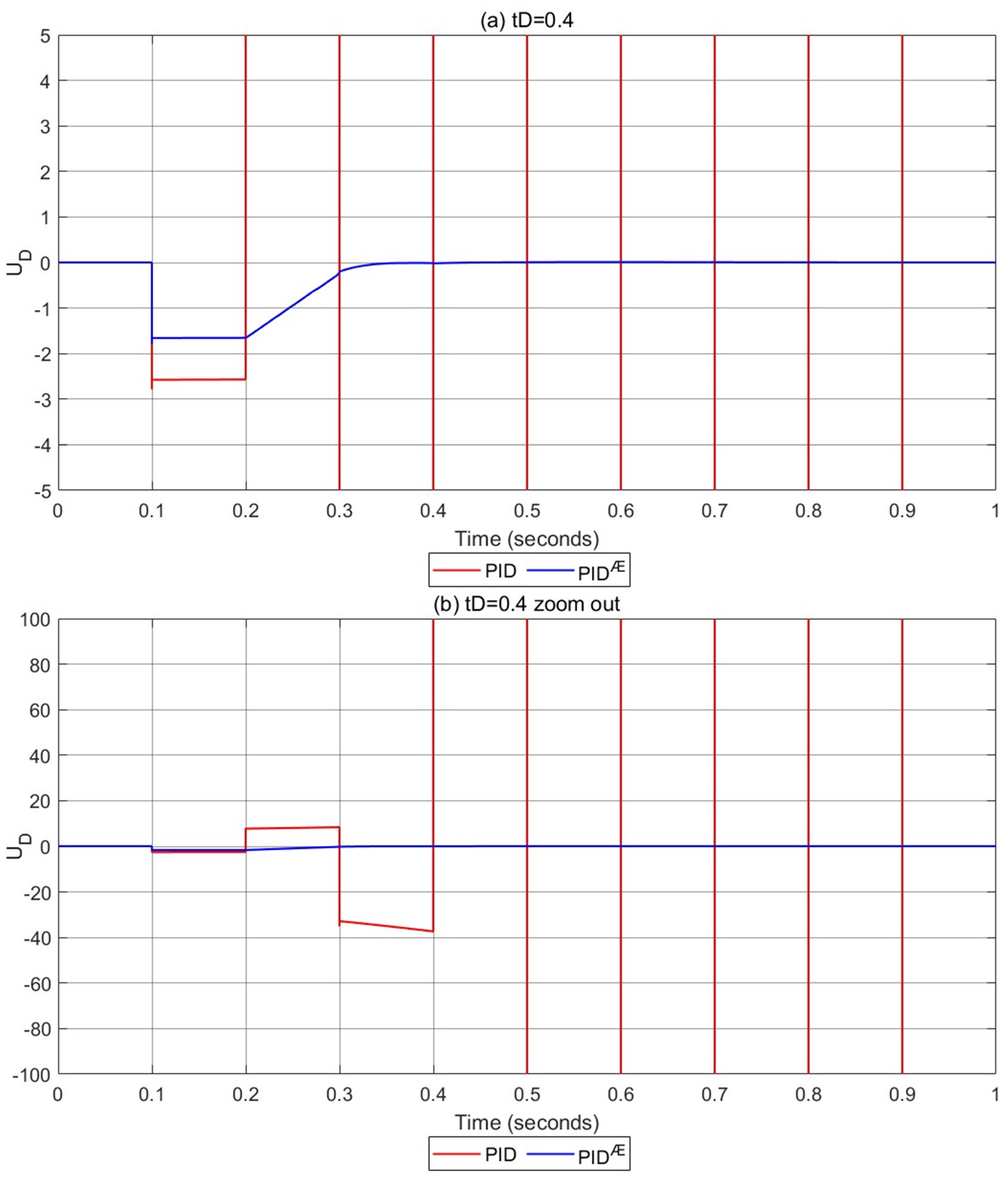
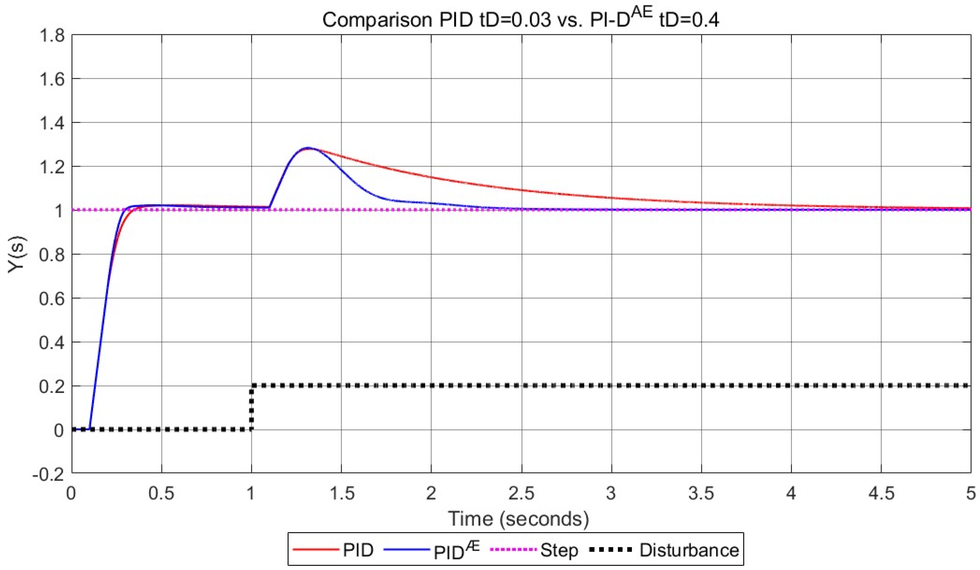
For higher values of (0.2 and 0.4), the PID controllers diverge, whereas - remains stable and delivers substantial performance improvements. Error accumulation metrics improve by up to 23%, while shows enhancements of up to 61%. Despite a slight increase in , the overall performance indicates faster and more-stable setpoint attainment with -. Additionally, shows minimal improvement at = 0.2 but is notably reduced by 53% at = 0.4. Importantly, decreases by up to 11.3% with -, ensuring better system stability.
-
dynamically adapts to
, effectively addressing issues such as instability and overshoot while accelerating response times.
Figure 3,
Figure 4,
Figure 5,
Figure 6,
Figure 7,
Figure 8,
Figure 9,
Figure 10,
Figure 11 and
Figure 12 confirm the superior robustness and disturbance rejection of
-
compared with
. Optimizing
mitigates instability, improves response acceleration, and ensures zero steady-state error, achieving enhanced system performance and reliability.
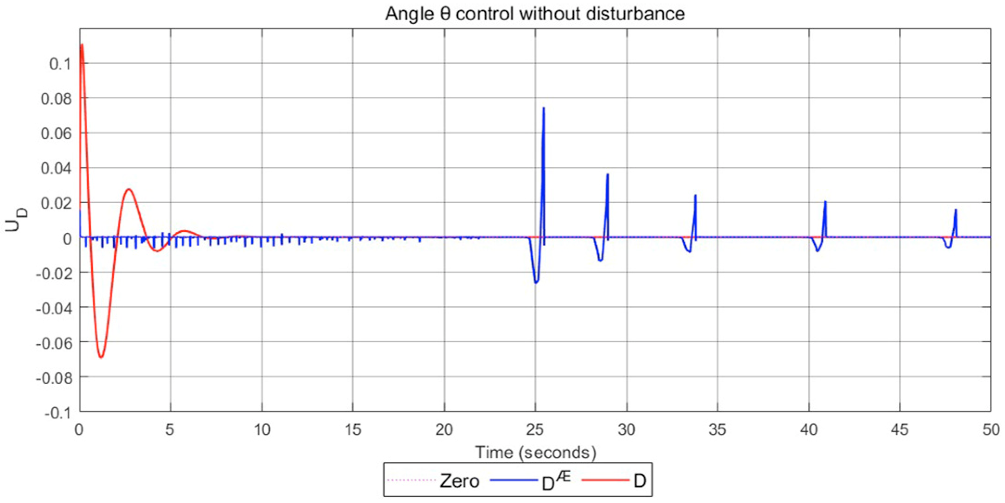
-
demonstrates significant advantages over
, particularly in equilibrium control. With identical
tuning,
-
achieves a near-zero steady-state error from the start, while
requires multiple oscillations before reaching stability. Notably,
-
effectively neutralizes
observed in
, as shown in
Figure 20, maintaining control over the θ angle with minimal oscillations and a stable signal.
Furthermore, -’s transient response exhibits unique characteristics. While its is faster, it achieves almost immediately, maintaining control near SP without oscillations. This contrasts with , which takes longer to stabilize. actively mitigates instability early on, as indicated by its initial high magnitude, compared with negligible activity in , which leads to pronounced .
Regarding and , - demonstrates a 99% reduction in , ensuring minimal overshoot and improved stability. Although occasional oscillations are present, their magnitudes are negligible, contributing to overall system robustness. The error accumulation metrics show significant improvements in three of four criteria, with only ITAE showing a slight increase, which remains inconsequential in absolute terms.
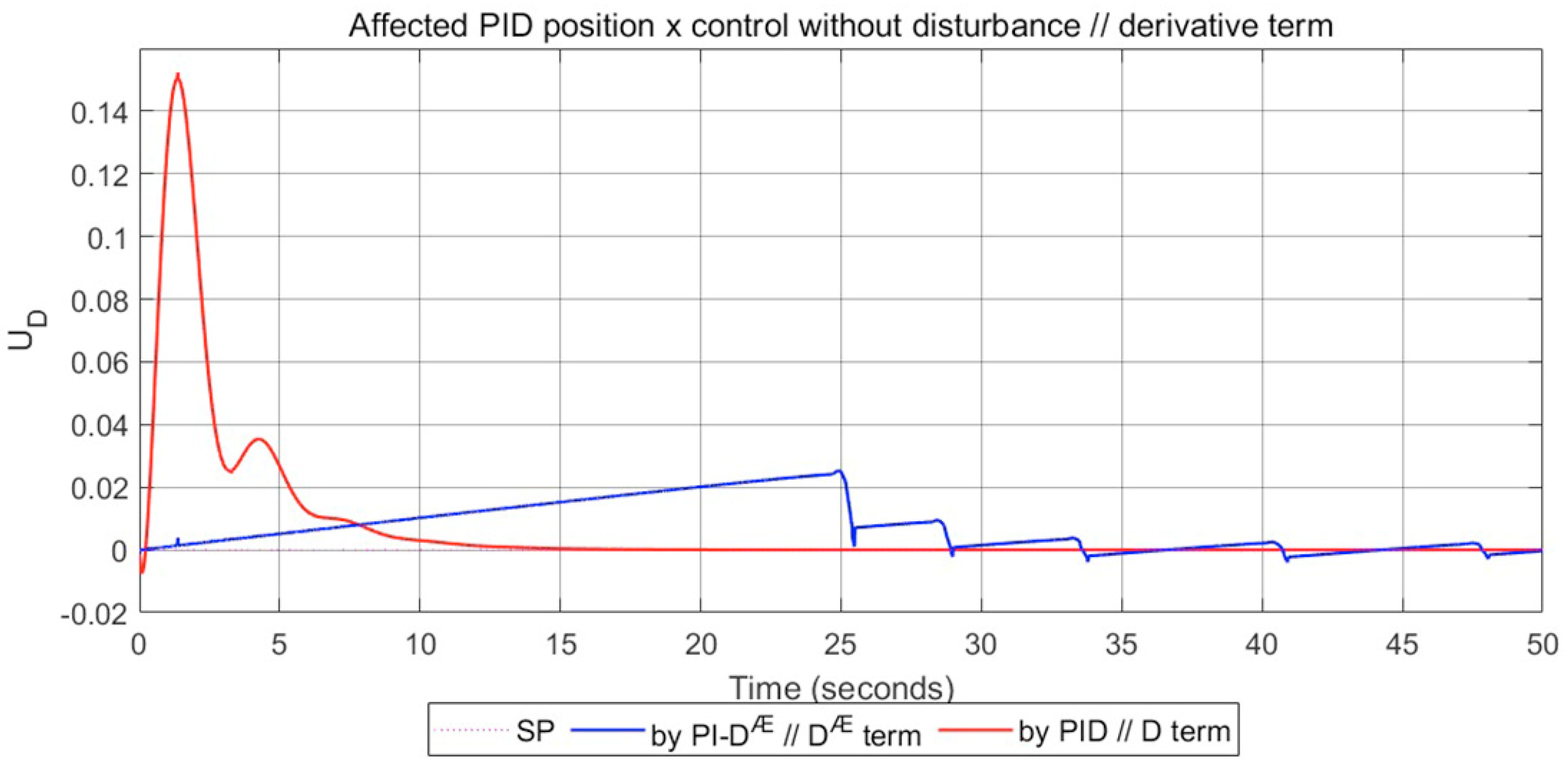
In the overlap analysis of equilibrium and position control signals (
Figure 18 and
Figure 19),
-
introduces slower transient responses and minor steady-state oscillations below SP. While this behavior slightly impacts position control, the primary focus of this study is equilibrium control.
-
demonstrates superior performance in stabilizing equilibrium by neutralizing
and enhancing robustness under dynamic conditions. These results confirm its effectiveness as a robust alternative to traditional
controllers, particularly for applications prioritizing stability and precision.
In IPC systems with disturbances, as shown in
Table 9 and
Table 10, the
-
controller significantly improved the control signal compared with PID and maintained low
magnitudes throughout the process. Error accumulation across all the criteria improved by over 82%, reaching up to 97% in the best case.
- achieved steady-state control from the start, while PID failed to reach equilibrium. Although for - was longer, the () overshoot was reduced by 99% relative to . Sub-impulses in the - response were minimal and acceptable when compared with , and the former consistently rejected oscillations and always maintained equilibrium.
The
-
controller stands out for its structural simplicity and computational efficiency, relying on only four parameters (Kp, Ki, Kd, and an adaptive exponent Æ) for implementation. In contrast to more-complex approaches such as FL PID controllers, which require 10 to 30 inference rules along with associated gain parameters, or NN-based PID controllers, which involve more than 20 parameters related to network architecture and training data, the
-
design does not require any prior training. Furthermore, while fuzzy and NN-based controllers entail medium and high computational costs, respectively, the
-
maintains a significantly low computational burden. Regarding performance, the
-
demonstrates high robustness to noise, comparable with that of NN-based controllers, yet with a considerably simpler and more direct implementation. [
18,
19,
20,
21,
22,
23,
24,
25]. These features make the
-
a highly effective and practical alternative for control systems in which operational efficiency and noise immunity are of critical importance.


 ,
, 


