Comparative Analysis of Artificial Neural Networks and Evolutionary Algorithms in DEA-β-MSV Portfolio Optimization

Abstract

This paper proposes a hybrid methodology for portfolio optimization by integrating the data envelopment analysis (DEA) model with the mean semivariance (MSV) framework. The goal is to construct portfolios that achieve targeted returns while minimizing downside risk. The methodology comprises two stages: (1) identifying efficient stocks through DEA, where semivariance and beta ($\beta$) are employed as input risk metrics and the expected return serves as the output, and (2) determining optimal portfolio weights through the MSV model, solved using artificial neural networks (ANNs) and evolutionary algorithms. The empirical results demonstrate that portfolios optimized with ANNs exhibit significantly lower risk compared to those derived from evolutionary algorithms, highlighting the superiority of ANN-based approaches in balancing risk and return under the proposed framework. This study underscores the potential of hybrid DEA-MSV models enhanced by machine learning techniques for advanced portfolio management.

1. Introduction

Portfolio optimization constitutes a substantial challenge within the realm of financial engineering, leading to the proliferation of various methodologies. Among these, the foundational mean variance (MV) model, as articulated by Markowitz [1], holds a position of paramount importance and lasting influence. The MV model addresses portfolio optimization by minimizing the portfolio risk subject to a target return or maximizing portfolio return subject to a defined risk tolerance. Building on this framework, Markowitz et al. [2] introduced the semivariance risk measure, arguing that its application results in the creation of portfolios that exhibit better performance relative to those constructed using variance. Subsequent research has focused on extending the mean semivariance (MSV) model to incorporate diverse real-world complexities. Huang [3] examined portfolio selection within a fuzzy environment, comparing fuzzy MV and MSV models and employing genetic algorithms for solution. Tsai and Wang [4] proposed the MSV model designed to manage uncertainty in both upside and downside risk and return. Qin et al. [5] modeled portfolio returns as fuzzy random variables, developed the MSV model with random returns, and implemented a hybrid solution algorithm. Gökgöz and Atmaca [6] optimized energy portfolios in the Turkish financial market, highlighting the influence of investor risk aversion on optimal solutions. Chen et al. [7] considered uncertain returns, transaction costs, cardinality, and boundary constraints within the MSV framework, and utilized evolutionary algorithms for solution. Hamdi et al. [8] addressed portfolio optimization under conditional value-at-risk (CVaR) by incorporating short selling, cardinality constraints, and transaction costs, and solved the resulting problem using penalty decomposition methods.

Traditional portfolio selection models primarily address unsystematic risk, exhibiting limitations in mitigating systematic risk. The beta criterion, which measures systematic risk, serves as a valuable complement to other risk measures, enhancing the overall risk management when used in combination. This is particularly relevant within the context of the capital asset pricing model (CAPM), which relates the expected return of a security to its beta risk. Researchers, including Chochola et al. [9], Chochola et al. [10], Hur and Chung [11], and Cenesizoglu and Reeves [12], have applied the CAPM model to analyze the dynamic of financial markets.

Given the vast number of assets in stock markets, the selection of efficient assets presents a significant challenge. Scientific methodologies are therefore imperative. The DEA method introduced by Charnes et al. [13] offers a non-parametric approach to assess the relative efficiency of decision-making units (DMUs) by comparing the ratio of their weighted outputs to weighted inputs. This methodology has been increasingly used in portfolio optimization. Morey and Morey [14] modeled the MV model using DEA, with variance as the input and the expected return as the output. Lamb and Tee [15] designed a skewness-MV model with DEA, evaluating mutual fund performance using variance as the input and return as the output. Branda [16] applied DEA to portfolio optimization, considering risk and return as the input and output, respectively. Xiao et al. [17] tackled the issue of uncertainty in stock returns and employed DEA for optimizing portfolios in the context of the American stock market. Zhou et al. [18] integrated DEA with multiple data sources to provide optimal portfolio support vector machines. Hamdi et al. [19] formulated a conditional risk model utilizing DEA and subsequently employed meta-heuristic algorithms for its resolution. Their research culminated in the presentation of an optimized portfolio within the Iranian stock market, demonstrating a propensity for efficient assets to receive maximal weighting within the portfolio construction.

This study aims to construct an optimal portfolio composed of efficient stocks from automotive companies while simultaneously managing the systematic risk. To this end, the MSV model is developed by integrating DEA with beta risk metrics. In contrast to traditional portfolio optimization approaches—such as mean variance or mean semivariance models that mainly depend on historical returns and risk measures like variance or semivariance—the proposed methodology assesses assets within a multidimensional analytical framework.

DEA incorporates multiple financial indicators, treating risk and financial leverage as inputs and metrics like return on equity, earnings per share, and the inverse price-to-earnings ratio as outputs. This approach provides a more comprehensive perspective on asset performance and financial health, facilitating the identification of assets that have not only generated favorable returns but are also fundamentally robust. When an asset (typically a company’s stock) is deemed fundamentally robust, it signifies that the issuing company possesses sound financial characteristics and indicators that suggest long-term stability, profitability, and growth potential. These attributes pertain to the company’s operational performance and intrinsic value, rather than solely its stock price in the market.

By allowing investors to prioritize criteria aligned with their objectives (e.g., earnings quality, valuation metrics, or capital structure), DEA enhances the portfolio selection process. As a result, the integration of DEA with the MSV model enables the construction of portfolios that excel not only in risk–return performance but also in foundational strength. This methodology transcends traditional optimization techniques by incorporating fundamental and operational factors, ensuring that selected assets operate efficiently and possess long-term growth potential.

Portfolio optimization problems highlight the limitations of traditional analytical techniques, which struggle to address non-linear objective functions, multiple constraints, and high-dimensional search spaces. These challenges render conventional approaches computationally inefficient or impractical in real-world scenarios. To overcome these shortcomings, the proposed methodology employs neural networks and multi-objective evolutionary algorithms (NSGA2 and SPEA2). Neural networks excel by learning intricate patterns in financial data, while evolutionary algorithms—inspired by natural selection—systematically explore vast solution spaces to identify near-optimal portfolios. This synergy enables the model to navigate the complexities of portfolio construction, prioritizing risk–return trade-offs and investor-specific criteria with greater adaptability and precision.

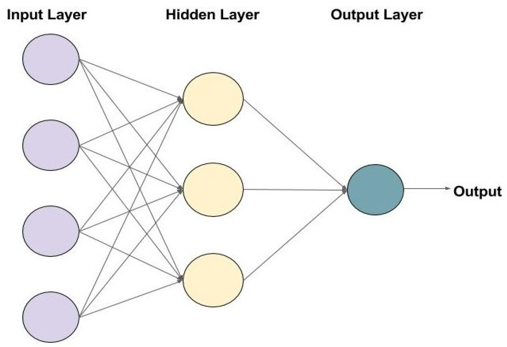
The remainder of this paper is organized as follows. Section 2 establishes the mathematical foundations of the DEA-$\beta$-MSV framework, detailing its components and theoretical principles. Section 3 follows with a comprehensive description of the feedforward neural network, emphasizing its architecture, training methodology, and adaptability to non-linear financial data for solving the optimization model. Section 4 then introduces the NSGA2 and SPEA2 algorithms, explaining their evolutionary mechanisms, parameter configurations, and integration into the multi-objective optimization workflow. Section 5 subsequently analyzes the empirical results derived from applying the proposed hybrid model to automotive sector portfolios, comparing the performance metrics across methodologies to evaluate their effectiveness. Finally, Section 6 synthesizes the key findings, discusses practical implications for portfolio management, and outlines potential directions for future research, reinforcing the study’s contributions to adaptive and robust investment strategies.

2. Mathematical Models

This section first presents the single-index model, then examines parametric optimization methods and DEA, before formally introducing the proposed model. Some assumptions are as follows:

• $\chi$ is a set of existing investment opportunities.
• ${\mathfrak{R}}_i$ is the return of i-th asset on the probability space $(\Omega ,F,P)$.
• ${\chi }^P=\{{\mathfrak{R}}_i:i=1,\dots ,n\}=\{{\sum }_{i=1}^n{\mathfrak{R}}_i{\epsilon }_i:{\sum }_{i=1}^n{\epsilon }_i=1,{\epsilon }_i\in \{0,1\}\}$. ${\epsilon }_i$ is the weight of each stock in the optimal portfolio.

Definition 1. 

Branda [20] Functionals $\nu :L^2\left(\Omega \right)\to \left[0,\infty \right]$ are designated as general deviation measures predicated upon their satisfaction of the following axiomatic properties: translation invariance, positive homogeneity, subadditivity, and non-negativity. These criteria are formally articulated as follows:

1. 

$\forall Y\in \chi ,\forall C\in \mathbb{R},\nu \left(Y+C\right)=\nu \left(Y\right).$

2. 

$\nu \left(0\right)=0,$ and $\forall Y\in \chi ,\forall \lambda >0,\nu \left(\lambda Y\right)=\lambda \nu \left(Y\right)$.

3. 

$\forall Y_1,Y_2\in \chi ,\nu \left(Y_1+Y_2\right)\le \nu \left(Y_1\right)+\nu \left(Y_2\right).$

4. 

$\forall Y\in \chi ,\nu \left(Y\right)\ge 0,$ with $\nu \left(Y\right)>0$ for non-constant $Y.$

It is pertinent to note that the axioms (2) and (3) jointly imply the convexity of such deviation measures. Prominent instantiations of this class include the standard deviation, the mean absolute deviation, and semideviations.

Definition 2. 

Branda [20] Functionals $\phi :L^2\left(\Omega \right)\to \left(-\infty ,\infty \right]$ are formally designated as return measures if and only if they satisfy a specific set of axiomatic properties: translation equivariance, positive homogeneity, superadditivity, and monotonicity. These conditions are rigorously defined as follows:

1. 

$\forall Y\in \chi ,\forall C\in \mathbb{R},\phi \left(Y+C\right)=\phi \left(Y\right)+C$.

2. 

$\phi \left(0\right)=0,and\forall Y\in \chi ,\forall \lambda >0,\phi \left(\lambda Y\right)=\lambda \phi \left(Y\right).$

3. 

$\forall Y_1,Y_2\in \chi ,\phi \left(Y_1+Y_2\right)\ge \phi \left(Y_1\right)+\phi \left(Y_2\right).$

4. 

$\forall Y_1,Y_2\in \chi ,$ if $Y_1\ge Y_2$ (in the pointwise sense), then $\phi \left(Y_1\right)\ge \phi \left(Y_2\right).$

It is pertinent to observe that axioms (2) and (3) jointly imply the concavity of the functional φ. The expectation operator is a fundamental example that demonstrably fulfills these axiomatic requirements. Furthermore, coherent risk measures, when subjected to scalar multiplication by a negative constant can be interpreted within the framework of return functionals.

2.1. Beta Risk

Systematic risk, an intrinsic element of the total return variability observed in securities, originates from pervasive market-wide shifts and developments. This form of risk, exerting influence across a broad spectrum of securities, encompassing both equities and bonds, is an unavoidable consequence of its direct correlation with fluctuations in interest rates, market volatility, and inflationary pressures. By way of illustration, a precipitous market downturn will typically induce a corresponding depreciation in the value of a multitude of equities, whereas a rapid market ascent will conversely precipitate price appreciation. The beta coefficient ($\beta$) is conventionally employed as an index for the quantification of a security’s systematic risk, and its computation proceeds as follows:

$${\beta }_i={\displaystyle \frac{Cov({\mathfrak{R}}_i,{\mathfrak{R}}_M)}{Var\left({\mathfrak{R}}_M\right)}},$$

(1)

where ${\mathfrak{R}}_i$ represents the return of the i-th stock, and ${\mathfrak{R}}_M$ denotes the market return. Market beta is conventionally set to one. Stocks with a beta greater than one typically exhibit a higher return volatility, whereas those with a beta less than one demonstrate lower return volatility.

2.2. Linear Representation of the Single Index Model

The single index model proposes a linear relationship to represent the return of a security, expressed as follows:

$${\mathfrak{R}}_i=A_i+{\beta }_{i}I+C_i,$$

(2)

where

• $A_i$ represents the expected return of stock i;
• ${\beta }_i$ quantifies the sensitivity of stock i to market movements (beta risk);
• $C_i$ is a random variable with an expected value of zero and variance ${\mathcal{Q}}_i$;
• I represents the level of a specific index. This index can encompass various macroeconomic or market-wide factors, such as the overall stock market level, Gross National Product, a price index, or any other singular factor considered to exert the most significant influence on security returns.

2.3. Standard Optimization

Consider a set $X\subseteq {\mathbb{R}}^n$ within the n-dimensional space that contains all the possible decision options, represented by vectors $\xi$. This set of valid options, X, is usually defined by constraints related to geometry, physical laws, and real-world limitations. We use a function $f:X\to {\mathbb{R}}^n$ to evaluate each of these decision options, assigning a real number that indicates its desirability. For our purposes here, we will focus on finding the option that minimizes the value of f, without losing generality, since maximizing f is equivalent to minimizing f. With this in mind, the standard optimization problem can be expressed as follows:

$$\begin{array}{c}\eta =\underset{\xi }{min}f\left(\xi \right)\hfill \\ s.t\xi \in X\subseteq {\mathbb{R}}^n.\hfill \end{array}$$

(3)

The goal is to identify a specific solution, represented as $\eta$, which corresponds to the minimum value of the objective function $f\left(\xi \right)$, where the possible choices for $\eta$ are within the feasible set X. Typically, mathematical optimization methods are employed to locate the extreme points (either local or global) of the function f.

2.4. Quadratic Programming Representation of Single Index Model

The return on an investment portfolio ($R_P$) is defined as the weighted sum of the returns of its constituent securities:

$$R_P=\sum _{i=1}^N{\epsilon }_i{\mathfrak{R}}_i,$$

where N is the number of assets and ${\epsilon }_i$ denotes the respective weighting of each asset within the portfolio. By substituting the single-index model (2) into this portfolio return equation, we obtain

$$R_P=\sum _{i=1}^N{\epsilon }_i\left(A_i+{\beta }_{i}I+C_i\right).$$

Following Sharpe [21], this can be further simplified to

$$R_P=\sum _{i=1}^{N+1}{\epsilon }_i\left(A_i+C_i\right).$$

Consequently, the expected return ($E\left[R_P\right]$) and portfolio risk ($Var\left[R_P\right]$) are determined as follows:

$$E\left[R_P\right]=\sum _{i=1}^{N+1}{\epsilon }_i{A}_i,$$

and

$$Var\left[R_P\right]=\sum _{i=1}^{N+1}{\epsilon }_i^2{\mathcal{Q}}_i.$$

Thus, the single index model naturally lends itself to a quadratic programming formulation, presented as

$$max \overline{\lambda }\sum _{i=1}^{N+1}{\epsilon }_i{A}_i-\sum _{i=1}^{N+1}{\epsilon }_i^2{\mathcal{Q}}_i$$

$$s.t\sum _{i=1}^N{\epsilon }_i=1,{\epsilon }_i\ge 0,$$

(4)

$$\sum _{i=1}^N{\epsilon }_i{\beta }_i={\epsilon }_{n+1},$$

where $\overline{\lambda }$ signifies the investor’s level of risk aversion, and ${\epsilon }_{n+1}$ represents the weighted average responsiveness of the portfolio return ($R_P$) to the level of the index (I).

2.5. Parametric Optimization

Parametric optimization involves finding the solution to a standard optimization problem, but this time, the solution is expressed as a function of certain parameters. These parameters are variables that are important for making decisions but cannot be directly controlled by the designer. Within the context of systems design, examples of parameters might include design specifications that have not been finalized, environmental factors, or characteristics of other interconnected parts of the system. Conceptually, solving a parametric search problem can be understood as applying standard optimization techniques for every possible combination of the parameter value(s). Let $\Lambda \subseteq {\mathbb{R}}^p$ represent the set of all feasible parameter vectors, ${\lambda }^{*}$. We can extend Equation (3) to handle this parametric scenario, as follows:

$$\begin{array}{c}\eta \left({\lambda }^{*}\right)=\underset{\xi }{min}f(\xi ,{\lambda }^{*})\hfill \\ s.t(\xi ,{\lambda }^{*})\le 0,\hfill \\ h(\xi ,{\lambda }^{*})=0,\hfill \\ {\lambda }^{*}\in \Lambda ,\hfill \\ \xi \in \mathrm{X}.\hfill \end{array}$$

When dealing with parametric optimization, the objective function is optimized considering the parameter vector as an input. Specifically, $\eta \left({\lambda }^{*}\right)$ represents the relationship between the parameter vector ${\lambda }^{*}$ and the minimum value of the objective function $f(\xi ,{\lambda }^{*})$ over all feasible $\xi \in X$. Consequently, the solution is not a single point but rather a set (which could be infinite). The constraints g and h are those that include both the design variables and the parameters.

The idea of parametric optimization has been explored in fields like economics by Carlsson and Korhonen [22], Milgrom and Segal [23], often with the goal of examining how solutions change in response to variations in one or a small number of parameter variables. This kind of analysis is valuable for understanding how a system behaves when faced with uncertain parameters. Examples include changes in market demands and prices in economics, or variations in boundary conditions and system properties in engineered systems. When these kinds of fluctuating conditions are incorporated into an optimization problem, a parametric optimization approach can be employed to analyze their impact on the resulting solution.

2.6. DEA Model

Suppose there are n DMUs with input vector $x_j=(x_{1j},\dots ,x_{mj})$ and output vector $z_j=(z_{1j},\dots ,z_{sj})$ where $z_j\ge 0,z_j\ne 0,x_j\ge 0,x_j\ne 0.$ Then, the DEA model in the nature of the input is as follows:

$$min \theta$$

$$s.t\sum _{i=1}^n{\varpi }_i{x}_i\le \theta x_{i0},i=1,\dots m,$$

$$\sum _{j=1}^n{\varpi }_j{z}_{rj}\ge z_{r0},r=1,\dots ,s,$$

(5)

$${\varpi }_j\ge 0,j=1,\dots ,n,$$

If $\theta =1$, then DMU is efficient, and if $\theta <1$, then DMU is inefficient.

In the basic DEA model, it is assumed that no specific relationship exists between inputs and outputs, and the model is non-parametric. Given our objective to extend this model for portfolio optimization, we introduce a specific assumption regarding the relationship between inputs and outputs. Since we define risk as the input and return as the output, and considering a linear relationship between these two variables, the proposed model will consequently be a parametric model.

Remark 1. 

In the DEA model, the input-oriented approach evaluates the efficiency of a DMU by assuming that the unit aims to minimize its inputs while keeping outputs constant. Conversely, the output-oriented approach in DEA assesses the DMU efficiency based on its endeavor to maximize its outputs while holding inputs constant. In the present study, we adopted a combined approach to determine the efficiency score. Specifically, we utilized the maximum efficiency value obtained from both the input-oriented and output-oriented calculations as the final efficiency index.

2.7. DEA Model for Risk Measurement

Consider a non-constant benchmark $Y_0$ belonging to the set $\chi$. Under the condition that ${\phi }_j\left(Y_0\right)$ for all $j\in \{1,\dots ,J\}$, with at least one index j satisfying this inequality, the DEA model for input-oriented risk (deviation) measurement is as follows:

$$min\theta$$

$$s.t.{\phi }_j\left(\sum _{i=1}^n{\epsilon }_i\left({\mathfrak{R}}_i\right)\right)\ge {\phi }_j\left(Y_0\right),j=1,\dots ,J,$$

$${\nu }_q\left(\sum _{i=1}^n{\epsilon }_i\left({\mathfrak{R}}_i\right)\right)\le \theta .{\nu }_q\left(Y_0\right),\mathrm{q}=1,\dots ,Q,$$

(6)

$$\sum _{i=1}^n{\epsilon }_i=1,{\epsilon }_i\ge 0,i=1,\dots ,n,$$

where $Y_0\in \chi$.

2.8. Input Attitude Models with Positive or Negative Data for Risk Measures

Let the DEA model take positive or negative input values, so that the basic DEA model changes as follows:

$$max\theta$$

$$s.t.{\phi }_j\left(\sum _{i=1}^n{\epsilon }_i\left({\mathfrak{R}}_i\right)\right)\ge {\phi }_j\left(Y_0\right)+\theta .{\pi }_j\left(Y_0\right),j=1,\dots ,J,$$

$${\nu }_q\left(\sum _{i=1}^n{\epsilon }_i\left({\mathfrak{R}}_i\right)\right)\le {\nu }_q\left(Y_0\right)-\theta .{\delta }_q\left(Y_0\right),\mathrm{q}=1,\dots ,Q,$$

(7)

$$\sum _{i=1}^n{\epsilon }_i=1,{\epsilon }_i\ge 0,i=1,\dots ,n,$$

where

$${\pi }_j\left(Y_0\right)=\underset{Y\in \chi }{max}\left({\phi }_j\left(Y\right)\right)-{\phi }_j\left(Y_0\right),$$

$${\delta }_q\left(Y_0\right)={\nu }_q\left(Y_0\right)-\underset{Y\in \chi }{min}{\nu }_q\left(Y\right).$$

This model identifies the inefficiency of investment opportunity $Y_0$. We can write that the objective function $\underset{\theta }{min}{\displaystyle \frac{1-\theta }{1+\theta }}$, so $Y_0$ is efficient if $\theta \left(Y_0\right)=1$; otherwise, it is inefficient.

2.9. MSV Model

Semivariance, also known as downside variance, is a statistical measure of the dispersion of returns for an asset or portfolio that specifically considers deviations below a defined target value. This metric is particularly relevant for evaluating the downside risk or the potential for significant losses in investments, as it disregards positive volatility (returns above the target), unlike standard variance. This risk measure is as follows.

Let ${\mathfrak{R}}_{ti}$ represent the return of the i-th security during period t, and let k denote the investment’s acceptable return threshold for the portfolio (target). Then, semivariance is defined as follows:

$$semivariance={\displaystyle \frac{1}{T}}\sum _{t=1}^T{\left[{\left(\sum _{i=1}^n{\mathfrak{R}}_{ti}{\epsilon }_i-k\right)}^{-}\right]}^2,$$

(8)

where

$${\left(\sum _{i=1}^n{\mathfrak{R}}_i{\epsilon }_i-k\right)}^{-}=\left\{\begin{array}{cc}{\displaystyle \sum _{i=1}^n}{\mathfrak{R}}_i{\epsilon }_i-k\hfill & {\displaystyle \sum _{i=1}^n}{\mathfrak{R}}_i{\epsilon }_i<k.\hfill \\ \\ 0\hfill & {\displaystyle \sum _{i=1}^n}{\mathfrak{R}}_i{\epsilon }_i\ge k.\hfill \end{array}\right.$$

So, the MSV model is as follows:

$$min{\displaystyle \frac{1}{T}}\sum _{t=1}^T{\left[{\left(\sum _{i=1}^n{\mathfrak{R}}_{ti}{\epsilon }_i-k\right)}^{-}\right]}^2$$

$$s.t \sum _{i=1}^M{\epsilon }_{i}E\left({\mathfrak{R}}_i\right)\ge E\left({\mathfrak{R}}_p\right),$$

(9)

$$\sum _{i=1}^M{\epsilon }_i=1,$$

$${\epsilon }_i\ge 0, i=1,\dots ,M,$$

where ${\mathfrak{R}}_p$ is the portfolio return and ${\epsilon }_i$ is the weight of i-th stock in the portfolio.

The adoption of semivariance as a risk measure, particularly in financial analysis and portfolio management, stems from the understanding that investors are often more concerned with the risk of losses than with the upside volatility. Consequently, semivariance can provide a more nuanced and pertinent assessment of the risk associated with unfavorable scenarios, informing more conservative investment decision-making.

2.10. DEA Model for $\beta$-MSV

Let $DMU=(\beta ,MSV).$ Then, the $\beta$-MSV model based on the DEA model is as follows:

$$max\theta$$

$$s.t.{\phi }_j\left(\sum _{i=1}^n{\epsilon }_i\left({\mathfrak{R}}_i\right)\right)\ge {\phi }_j\left(Y_0\right)+\theta .{\pi }_j\left(Y_0\right),j=1,\dots ,J,$$

$$MS{V}_q\left(\sum _{i=1}^n{\epsilon }_i\left({\mathfrak{R}}_i\right)\right)\le MS{V}_q\left(Y_0\right)-\theta .{\delta }_q\left(Y_0\right),\mathrm{q}=1,\dots ,Q,$$

$${\beta }_q\left(\sum _{i=1}^n{\epsilon }_i\left({\mathfrak{R}}_i\right)\right)\le {\beta }_q\left(Y_0\right)-\theta .{\widehat{\delta }}_q\left(Y_0\right),\mathrm{q}=1,\dots ,Q,$$

(10)

$$\sum _{i=1}^n{\epsilon }_i=1,{\epsilon }_i\ge 0,i=1,\dots ,n.$$

where

$${\pi }_j\left(Y_0\right)=\underset{Y\in \chi }{max}\left({\phi }_j\left(Y\right)\right)-{\phi }_j\left(Y_0\right),$$

$${\delta }_q\left(Y_0\right)=MS{V}_q\left(Y_0\right)-\underset{Y\in \chi }{min}MS{V}_q\left(Y\right).$$

$${\widehat{\delta }}_q\left(Y_0\right)={\beta }_q\left(Y_0\right)-\underset{Y\in \chi }{min}{\beta }_q\left(Y\right).$$

Remark 2. 

In accordance with Remark (1), an efficient stock is characterized in this study by its capacity to yield the minimum risk for a particular level of return, or conversely, to provide a high return for a given level of risk. This characterization similarly holds true for efficient portfolios.

Proposition 1. 

Consider the optimization problem,

$$\underset{\omega \in {\mathbb{R}}^n}{min}E{\left[{(\alpha +\omega {\varphi }^{\prime })}^{-}\right]}^2,$$

(11)

where the sentence ${(\alpha +\omega {\varphi }^{\prime })}^{-}=min((\alpha +\omega {\varphi }^{\prime }),0)$. ${\varphi }^{\prime }$ is the transpose of the matrix $\varphi =({\varphi }_1,\dots ,{\varphi }_n)$, w is the asset weight vector, and α, ${\varphi }_i$, $i=1,\dots ,n$ are random variables by $E\left[{\alpha }^2\right]<\infty ,E\left[{\varphi }_i^2\right]<\infty$. If $E\left[{\varphi }_i\right]=0,$ for all i, then the problem (11) accepts a solution.

Proof. 

The proof of Proposition 1 can be found in Jin et al. [24]. □

Proposition 2. 

Suppose the initial capital is γ such that ${\sum }_{i=1}^n{\epsilon }_i=\gamma$ and $\theta \le 1.$ Then, for any expected return of the portfolio, problem (10) has an optimal solution if it embraces feasible solutions.

Proof. 

We can rewrite the problem (10) as follows:

$$min{\displaystyle \frac{1}{T}}\sum _{t=1}^T{\left[{\left(\sum _{i=1}^n{\mathfrak{R}}_{ti}{\epsilon }_i-k\right)}^{-}\right]}^2$$

$$s.t.{\phi }_j\left(\sum _{i=1}^n{\epsilon }_i\left({\mathfrak{R}}_i\right)\right)\ge {\phi }_j\left(Y_0\right)+\theta .{\pi }_j\left(Y_0\right),j=1,\dots ,J,$$

$${\displaystyle \frac{2}{1+\theta }}-1\ge 0,$$

$${\beta }_q\left(\sum _{i=1}^n{\epsilon }_i\left({\mathfrak{R}}_i\right)\right)\le {\beta }_q\left(Y_0\right)-\theta .{\widehat{\delta }}_q\left(Y_0\right),\mathrm{q}=1,\dots ,Q,$$

(12)

$$\sum _{i=1}^n{\epsilon }_i=1,{\epsilon }_i\ge 0,i=1,\dots ,n,$$

where

$${\pi }_j\left(Y_0\right)=\underset{Y\in \chi }{max}\left({\phi }_j\left(Y\right)\right)-{\phi }_j\left(Y_0\right),$$

$${\widehat{\delta }}_q\left(Y_0\right)={\beta }_q\left(Y_0\right)-\underset{Y\in \chi }{min}{\beta }_q\left(Y\right).$$

Since the maximum value of $\theta$ occurs in $0\le \theta \le 1$, constraint ${\displaystyle \frac{2}{1+\theta }}-1\ge 0$ is guaranteed. Also, the following constraint,

$$MS{V}_q\left(\sum _{i=1}^n{\epsilon }_i\left({\mathfrak{R}}_i\right)\right)\le MS{V}_q\left(Y_0\right)-\theta .{\delta }_q\left(Y_0\right),$$

in problem (10), means the lowest amount of the MSV for the highest $\theta$. Hence, the objective function of problem (12) is guaranteed.

Now, let $r_i$ and ${\mu }_i$ be the return and expected return, respectively. Then, the objective function of problem (12) can be written as follows:

$$E{\left[{\left(\sum _{i=1}^n{\epsilon }_i{r}_i-\sum _{i=1}^n{\epsilon }_i{\mu }_i\right)}^{-}\right]}^2=E{\left[{\left(\sum _{i=1}^n{\epsilon }_i(r_i-{\mu }_i)\right)}^{-}\right]}^2.$$

We set ${\mathfrak{R}}_i=r_i-{\mu }_i$. Then, based on the initial capital, we have for asset 1

$${\epsilon }_1=\gamma -\sum _{i=2}^n{\epsilon }_i,$$

so

$$E{\left[{\left(\gamma {\mathfrak{R}}_1-\sum _{i=1}^n{\epsilon }_i{\mathfrak{R}}_1+\sum _{i=1}^n{\epsilon }_i{\mathfrak{R}}_i\right)}^{-}\right]}^2=E{\left[{\left(\gamma {\mathfrak{R}}_1+\sum _{i=1}^n{\epsilon }_i({\mathfrak{R}}_i-{\mathfrak{R}}_1)\right)}^{-}\right]}^2.$$

Then, the objective function of problem (12) is as follows:

$$min E{\left[{\left(\gamma {\mathfrak{R}}_1+\sum _{i=1}^n{\epsilon }_i({\mathfrak{R}}_i-{\mathfrak{R}}_1)\right)}^{-}\right]}^2.$$

Let ${\mathfrak{R}}_i={\mathfrak{R}}_1$. Then, optimal solutions are admitted by Proposition 1. □

3. Artificial Neural Network

Artificial intelligence (AI), as a broad field, aims to develop systems capable of emulating human intelligence. A pivotal approach in realizing this objective is machine learning. Machine learning involves the utilization of algorithms that enable systems to learn from data without explicit programming and autonomously enhance their performance. Neural networks (NNs), inspired by the architecture of the human brain, constitute a potent class of machine learning models and are employed in numerous advanced applications of artificial intelligence. Subsequently, this discussion will delve into a more detailed examination of a significant type of neural network, namely, feedforward neural networks. These computational structures, drawing inspiration from the operational principles of the human brain, are utilized for learning patterns inherent in data. This section will explore the mathematical underpinnings of these networks and introduce the fundamental formulas that govern their behavior across various layers (input, hidden, and output). Figure 1 shows a feedforward neural network with one hidden layer.

3.1. Feedforward Neural Network for Portfolio Semivariance Prediction

This section details the architecture of a feedforward neural network designed to predict a portfolio’s semivariance.

1. Inputs and Outputs:

• Network Input: The input layer receives the weights of the assets in the portfolio.
• Network Output: The output layer, consisting of a single neuron, predicts the portfolio’s semivariance, which is a continuous value.

2. Architecture and Neurons

The network features three hidden layers with 30, 20, and 10 neurons, respectively.

• Weights (${\mathit{\vartheta }}_{\mathit{ji}}$) and Biases (${\mathit{b}}_{\mathit{j}}$): These are randomly initialized and then adjusted during the learning process using the backpropagation algorithm to minimize prediction error.
• Activation Functions:

  –

  Hidden Layers: We employ the hyperbolic tangent sigmoid (tansig) function, defined as $\psi \left(d\right)={\displaystyle \frac{1}{1+e^{-d}}}$. This function compresses the output into the range $(0,1)$.

  –

  Output Layer: For this regression problem, a linear function (purelin) is used.

• Summation Function: The weighted sum of inputs for each neuron is automatically calculated using

  $$c_j=\sum _{i=1}^n{\vartheta }_{ji}{d}_i+b_j.$$

3. Learning Process: Backpropagation

The learning and training process begins by feeding the network the asset weights (input) and the corresponding semivariance (output).

• Cost Function ($\mathit{J}\left(\mathbf{\Theta }\right)$): The training function implicitly uses a cost function, typically the mean squared error (MSE), to quantify the difference between the network’s predicted semivariance and the actual semivariance. The primary goal of training is to minimize this cost function.
• Backpropagation Algorithm: This algorithm is implemented within the training function and involves two main passes:

  –

  Forward Pass: The asset weights are propagated through the network to generate the predicted semivariance.

  –

  Backward Pass: The error at the output layer is calculated. Subsequently, the gradients of the cost function with respect to all weights and biases across all layers are computed in reverse (from the output layer towards the input layer).

• Weight and Bias Updates: These calculated gradients are used to update the weights and biases (e.g., ${\vartheta }_{ji}^{\left(l\right)}={\vartheta }_{ji}^{\left(l\right)}-\kappa {\displaystyle \frac{\partial J\left(\mathsf{\Theta }\right)}{\partial {\vartheta }_{ji}^{\left(l\right)}}}$) using an optimization algorithm such as Levenberg–Marquardt. The learning rate $\kappa$ is an internal parameter of these optimization algorithms that governs the size of each update step.

3.2. Regularization: Early Stopping

Early stopping is a crucial technique in training machine learning models, particularly neural networks. Its primary purpose is to prevent overfitting and ensure the model’s better generalization capability on new, unseen data. During the training process, a model endeavors to minimize its error on the training data. However, excessive training can lead the model to “memorize” noise and specific characteristics of the training data rather than learning general patterns. This phenomenon is known as overfitting. An overfit model performs exceptionally well on data it has previously encountered but struggles with predictions on new and unknown data. Early stopping helps mitigate this issue. To implement early stopping, the original dataset is typically divided into three distinct subsets:

• Training set: This dataset is used to train the machine learning model, allowing it to adjust its parameters (e.g., weights in a neural network).
• Validation set: This portion of the data is used to monitor the model’s performance during the training process. The model does not train on this data; instead, its performance is merely evaluated on it. This monitoring indicates how well the model can generalize to new data.
• Test set: This dataset is kept completely separate and is only used at the end of the training process for a final, unbiased evaluation of the model’s performance.

The early stopping process unfolds as follows. In each training step (or “epoch”), the model’s error is calculated on both the training and validation data. Initially, both errors are expected to decrease. As training progresses, the training error may continue to decline (as the model memorizes the data), but at some point, the validation error will begin to increase. This inflection point signifies the onset of overfitting. Early stopping is triggered when the validation error increases for a specified number of consecutive epochs. At this juncture, training is halted, and typically, the model’s best parameters (weights and biases) from the epoch where the validation error was at its minimum are selected and saved.

4. Meta-Heuristic Algorithms

In this section, we introduce two prominent multi-objective evolutionary algorithms, NSGA2 and SPEA2, to solve the portfolio optimization problem. Both algorithms are designed to handle multiple conflicting objectives, such as maximizing the expected return while minimizing risk and transaction costs.

4.1. NSGA2 Algorithm

The genetic algorithm (GA) constitutes a robust stochastic search methodology, emulating the principles of natural selection. This algorithm integrates Darwinian principles of survival with structured random information, thereby constructing a search algorithm wherein, during each generation, the fittest individuals are selected, rather than solely the optimal ones. The GA is an iterative process designed to identify optimal solutions, manipulating a population of fixed size. The procedural steps of this algorithm are delineated as follows.

• Creating an initial population of size N.
• Calculation of objective function values.
• Sorting the answers based on dominance and crowding distance.
• Selection of parents, the act of crossing, and creating a population of children.
• Selection of parents, mutation, and creation of the population of mutants.
• Combining the new population with the original population.
• Selecting members of the new main population with size N based on dominance and crowding distance.
• If the termination conditions are not met, the second step, and, otherwise, the end.

4.2. SPEA2 Algorithm

SPEA2 uses a regular population and an archive. In this algorithm, a power value is assigned to each non-dominant answer. The power value is represented by $A\left(i\right)$. The following are defined in this algorithm.

Primary population $B_0$, main population in repetition $B_{\ell }$, archive primary population ${\overline{B}}_0$, archive population in replication ${\overline{B}}_{\ell }$, the number of members of the main population $\left|B_{\ell }\right|=N$, and number of archive population members in replication $\left|{\overline{B}}_{\ell }\right|=\overline{N}$.

At first, each member i of the population $B_{\ell }\cup {\overline{B}}_{\ell }$ is assigned a power value with the symbol $A\left(i\right)$. $A\left(i\right)$ is the number of members of the population or archive that are defeated by i.

That is, $A\left(i\right)=\left|\left\{i\left|i\in B_{\ell }\cup {\overline{B}}_{\ell }\wedge i>j\right.\right\}\right|, i\in B_{\ell }\cup {\overline{B}}_{\ell }.$

Raw Fitness

The total value of the strength of the members of the population for which i is defeated is called the raw fitness.

$$V\left(i\right)=\sum _{j\in B_{\ell }\cup {\overline{B}}_{\ell },i>j}A\left(j\right).$$

$V\left(i\right)$ is an integer. In SPEA2, the more that answers are defeated by a stronger answer (the answer that overcomes more members of the population), the higher their raw fitness value will be, and in SPEA2, an answer that has a lower raw fitness is considered. That is, the less dominant answer has a higher chance of being selected. If two or more answers are the same (having the same rank but in a different distribution), then density fitting is used for the preferred answer. The fitness is calculated using the following formula:

$$F\left(i\right)=V\left(i\right)+W\left(i\right),$$

where

$$W\left(i\right)={\displaystyle \frac{1}{{\sigma }_i^u+2}}, u=\sqrt{N+\overline{N}}.$$

The value of $\sigma$ represents the distance of each person from their u-th nearest neighbor.

To select parents and control the archival population, if $\left|{\overline{B}}_{\ell +1}\right|<\overline{N}$, $B_t$ dominant members are used to populate the population. In this method, members with better fitness are used. Unlike the classical genetic algorithm, where the new population, or the final population, is created by merging the three populations, mutation and combination, and the previous population, in SPEA2, the new population is created by the integration of the population resulting from mutation and combination, and the initial population does not affect it.

4.3. Constraint Handling in Evolutionary Optimization Problems

Section 5 details the application of the aforementioned evolutionary algorithms to solve model (12), specifically addressing the constraints ${\sum }_{i=1}^n{\epsilon }_i=1$ and ${\epsilon }_i\ge 0$. Consequently, this section elucidates the methodology by which these algorithms accommodate such constraints. Both NSGA2 and SPEA2, as general-purpose multi-objective evolutionary algorithms, inherently lack specific internal mechanisms for directly handling constraints within their foundational formulations. Consequently, their application to constrained optimization problems necessitates reliance on external constraint management techniques. For the portfolio optimization problem, which is characterized by simplex feasibility constraints—namely, the non-negativity of individual weights (${\epsilon }_i\ge 0$) and the requirement that the sum of all weights equals one (${\sum }_{i=1}^n{\epsilon }_i=1$)—we implemented a two-pronged repair-based approach, as follows:

• Non-Negativity of Weights (${\mathit{\epsilon }}_{\mathit{i}}\mathbf{\ge }\mathbf{0}$): This constraint was enforced through a repair mechanism applied during the population generation process. Specifically, any portfolio weight that became negative as a result of genetic operators (crossover and mutation) was immediately set to zero. This procedure guarantees that all candidate solutions consistently adhere to the non-negativity requirement.
• Sum of Weights Equals One (${\sum }_{\mathit{i}\mathbf{=}\mathbf{1}}^{\mathit{n}}{\mathit{\epsilon }}_{\mathit{i}}\mathbf{=}\mathbf{1}$): This critical constraint was meticulously managed by a dedicated normalization operator. Following the application of crossover and mutation, which can generate offspring with a sum of weights not equal to one, a normalization step was performed. In this step, the sum of all generated weights (which had already undergone the non-negativity repair) was computed, and subsequently, each individual weight was divided by this calculated sum. This iterative process ensures that the sum of weights for every portfolio precisely equals one in every generation. This repair operation is applied immediately after offspring production in each generation, thereby guaranteeing that every individual evaluated and propagated to the subsequent generation constitutes a valid portfolio conforming to the simplex feasibility constraints.

5. Application: Iran Stock Market

This research employs an applied methodology, utilizing quantitative data within a post-event framework and drawing upon historical data from automotive enterprises. Data was collected via archival retrieval from stock exchange repositories. The statistical sample comprises data from 21 automotive firms over the period of 2017 to 2021. The selection of the Iranian automotive industry for this study was driven by several compelling factors. It represents a large and strategically important sector within Iran’s economy, characterized by substantial transaction volumes and a rich availability of data, including stock prices, returns, and financial information. Furthermore, the industry’s inherent high volatility and considerable susceptibility to economic policies present a challenging yet fertile ground for the rigorous testing of financial models. This dynamism provides a realistic scenario for evaluating model performance under complex market conditions. Finally, the chosen period of 2017–2021 was critical as it yielded a robust and comprehensive dataset suitable for both model training and testing, unlike preceding or subsequent periods, which contained incomplete or less pertinent data.

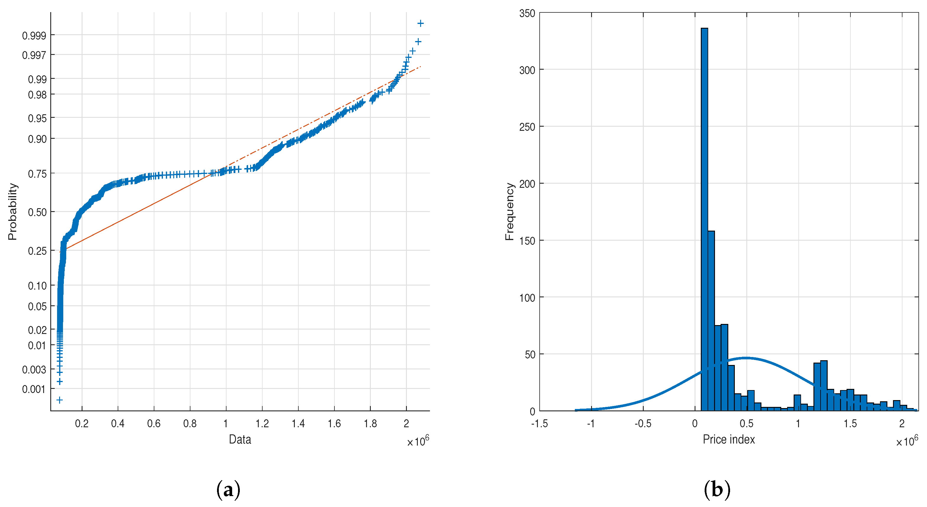
Statistical computations and model implementation were performed utilizing MATLAB software. Market evaluation commenced with an analysis of the automotive market index, as illustrated in Figure 2. Observations indicate a non-normal distribution of the market index. Further analysis, through the construction of a histogram, revealed a positive skew, as evidenced in Figure 2. This positive skewness suggests a potential for future appreciation in the automotive price index, implying opportunities for substantial returns for market participants. Subsequently, the statistical sample underwent analysis to ascertain the beta risk, semivariance risk, and expected returns for each stock.

Subsequently, the statistical sample underwent analysis to calculate the beta risk, semivariance risk, and expected returns for each stock from Equations (1), (8), and (13).

$$\phi \left[\mathfrak{R}\right]=E\left[\mathfrak{R}\right]={\displaystyle \frac{1}{n}}\sum _{i=1}^n{\mathfrak{R}}_i\left({\mathfrak{R}}_{i}isthedailyreturn\right).$$

(13)

Additional details on the computation of daily returns and semivariance can be found in Appendix A.

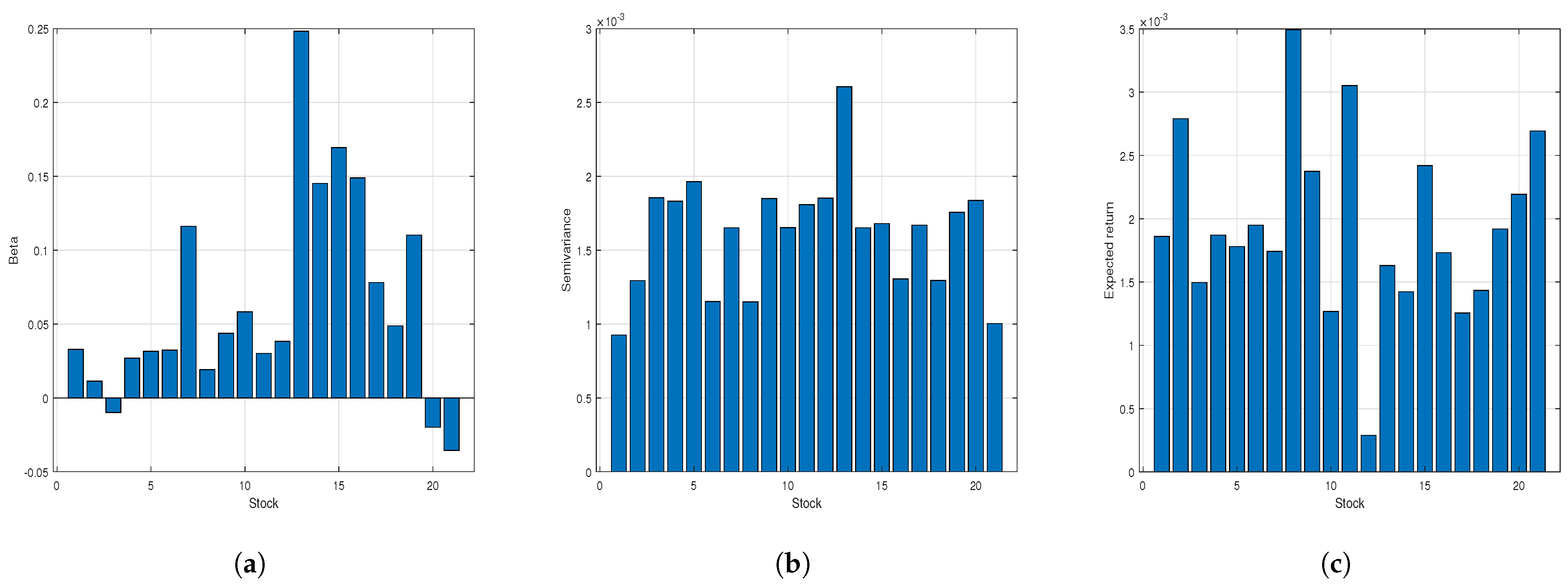
The respective values for $\beta$, semivariance, and expected returns are presented in Figure 3. In Figure 3, the negative beta observed in certain stocks within automotive companies indicates a negative covariance between the returns of these stocks and the automotive market index. In other words, these stocks tend to move in the opposite direction of the automotive market. Consequently, the inclusion of such stocks in an automotive investment portfolio can mitigate the portfolio’s systematic risk. Furthermore, according to Figure 3, stock #21 exhibits the lowest beta risk, while stock #1 demonstrates the lowest semivariance. Conversely, stock #8 presents the highest expected return.

The proposed model (10) introduces a new parametric optimization approach, building on DEA. Its input parameters include $\phi$ (expected return), $MSV$ (semivariance risk), and $\beta$ (market risk). This model uniquely applies DEA to conceptualize risk as a consumed resource (input) and return as a generated product (output), enabling an evaluation of individual assets’ relative efficiency in converting risk into return. The utilization of beta risk, in conjunction with semivariance risk, facilitates a more nuanced assessment of an asset’s efficiency by incorporating systematic market risk. Assets demonstrating superior return generation for a given level of risk, or conversely, exhibiting lower risk for a given level of return, are identified as relatively more efficient and consequently receive higher efficiency scores, approaching unity. Conversely, assets exhibiting comparatively lower returns relative to their incurred risk, when juxtaposed with other assets within the dataset, are deemed inefficient and are assigned lower efficiency scores. The application of DEA efficiency scores enables the identification and subsequent exclusion of inefficient assets from a portfolio. After solving model (10), its results were presented in Table 2.

As evidenced in

Table 1. Input and output consist of the $\beta$, semivariance, and expected return.

		Inputs		Output
Asset ID	Stock Companies	$\mathit{\beta }$	Semivariance	Expected Return
1	CHAR1	0.0329	0.0009	0.0019
2	FNAR1	0.0113	0.0013	0.0028
3	GOST1	−0.0099	0.0019	0.0015
4	IKCO1	0.0269	0.0018	0.0019
5	KFAN1	0.0316	0.0020	0.0018
6	KHSH1	0.0323	0.0012	0.0020
7	KRIR1	0.1162	0.0017	0.0017
8	LENT1	0.0191	0.0012	0.0035
9	MESI1	0.0438	0.0018	0.0024
10	MHKM1	0.0583	0.0017	0.0013
11	MNSR1	0.0301	0.0018	0.0031
12	MSTI1	0.0383	0.0019	0.0003
13	NMOH1	0.2483	0.0026	0.0016
14	PKOD1	0.1452	0.0017	0.0014
15	RADI1	0.1694	0.0017	0.0024
16	RIIR1	0.1490	0.0013	0.0017
17	RTIR1	0.0781	0.0017	0.0013
18	SIPA1	0.0488	0.0013	0.0014
19	SZPOL1	0.1102	0.0018	0.0019
20	TMKH1	−0.0199	0.0018	0.0022
21	ZMYD1	−0.0356	0.0010	0.0027

, with the exception of stock #8, the expected returns of the remaining stocks exhibit relative homogeneity. Consequently, as illustrated in

Table 2. Efficiency of any stock.

Asset ID	Stock Companies	Efficiency
1	CHAR1	1
2	FNAR1	0.8258
3	GOST1	0.5222
4	IKCO1	0.5355
5	KFAN1	0.5096
6	KHSH1	0.8101
7	KRIR1	0.5607
8	LENT1	1
9	MESI1	0.6796
10	MHKM1	0.5606
11	MNSR1	0.8737
12	MSTI1	0.5080
13	NMOH1	0.4667
14	PKOD1	0.5607
15	RADI1	0.6928
16	RIIR1	0.7094
17	RTIR1	0.5546
18	SIPA1	0.7155
19	SZPOL 1	0.5493
20	TMKH1	0.7502
21	ZMYD1	1

, the DEA model identifies this particular stock as efficient due to its comparatively high return. Notably, this elevated return is achieved in conjunction with low semivariance, indicative of the stock’s inherent quality. In Table 1, stock #1 demonstrates a markedly low semivariance; hence, it attains an efficiency score of 1.0 in Table 2. Furthermore, stock #21 achieves an efficiency score of 1.0 in Table 2, owing to its simultaneously low market risk and semivariance. This concurrent low level of both risk metrics for this specific stock suggests a robust underlying company performance. In environments characterized by market uncertainty, the prediction of future returns becomes increasingly complex, and risk profiles can exhibit rapid fluctuations. DEA, by evaluating the efficiency of assets in converting contemporaneous risk into contemporaneous return, offers a relatively dynamic analytical perspective. This facilitates the identification of assets that have, historically, demonstrated a superior performance relative to their accepted risk under prevailing market conditions. Moreover, the integration of beta risk alongside semivariance assists investors in considering systematic market risk in addition to downside volatility risk (semivariance). In uncertain market conditions, systematic risk can assume a more prominent role, rendering its consideration crucial for comprehensive portfolio risk management.

Furthermore, the selection of assets that exhibit efficiency in converting risk into return can indirectly lead to the inclusion of companies with stronger fundamental characteristics. Entities demonstrating greater stability and profitability are more likely to exhibit resilient performance in uncertain market conditions. Additionally, in volatile market environments, the identification and subsequent removal of assets characterized by low returns relative to their associated risk assumes heightened importance. DEA, through the provision of a quantitative efficiency score, offers investors a valuable tool for this specific purpose.

While DEA evaluates contemporaneous performance, its computation of risk and return is inherently predicated on historical data. Given the potential for past efficiency to become an unreliable predictor of future outcomes due to abrupt market shifts, it is crucial to recognize DEA as a tool for ex-post performance evaluation rather than a mechanism for forecasting. This methodology lacks the inherent capacity to directly anticipate future market fluctuations. The DEA method serves to delineate the relative efficiency of assets; however, it does not directly furnish optimal weightings for portfolio construction.

Our analysis successfully identifies efficient assets; however, allocating capital among them necessitates additional methodologies. Consequently, our subsequent goal is to determine optimal weights for these efficient stocks by solving model (12) through two different techniques: neural networks and evolutionary algorithms. The specific parameter configurations for the NSGA2 and SPEA2 algorithms can be found in

Table 3. Inputs of NSGA2.

Algorithm 1. NSGA2	Factor
Maximum Number of Iterations	100
Population Size	50
Archive Size	100
Crossover Percentage	0.7
Mutation Percentage	0.3
Mutation Rate	0.02

and

Table 4. Inputs of SPEA2.

Algorithm 2. SPEA2	Factor
Maximum Number of Iterations	100
Population Size	50
Archive Size	100
Crossover Percentage	0.7
Mutation Percentage	0.3

, respectively. It is crucial to distinguish that while the previous step established efficient shares considering all input and output constraints, we now simplify the problem by applying only the ${\sum }_{i=1}^n{\epsilon }_i=1,{\epsilon }_i\ge 0$ constraint, thereby solving a dedicated portfolio optimization problem using these advanced methods.

Neural networks, particularly multilayer perceptrons, exhibit substantial efficacy in discerning non-linear patterns and intricate interrelationships within financial datasets. They can effectively exploit the stock efficiency metrics derived from DEA to discern underlying regularities.

We address the semivariance model for three efficient stocks using a neural network. We designed a feedforward neural network with three hidden layers. The input layer handles 1000 prospective weight vectors, while the output layer estimates portfolio semivariance. The mapping function from 1000 probable weight vectors to a portfolio’s semivariance is inherently complex and non-linear. Consequently, the accurate learning of this function necessitates a network architecture beyond one or two hidden layers. This intrinsic complexity, rather than input dimensionality, determines the requisite network depth. Insufficient depth, evidenced by unsatisfactory performance, signals underfitting, for which augmenting network depth by adding more hidden layers is a suitable solution. Three hidden layers were employed, providing sufficient depth to extract abstract features from weight combinations. Neuron counts of 30, 20, and 10 were selected for these layers, respectively. This decision stemmed from suboptimal performance with fewer neurons, as lower counts reduce model capacity, hindering accurate approximations of the semivariance function. A decreasing neuron count across layers is a common and effective neural network architecture. To prevent overfitting, early stopping was implemented; training halted if the validation error worsened for six consecutive epochs without improvement.

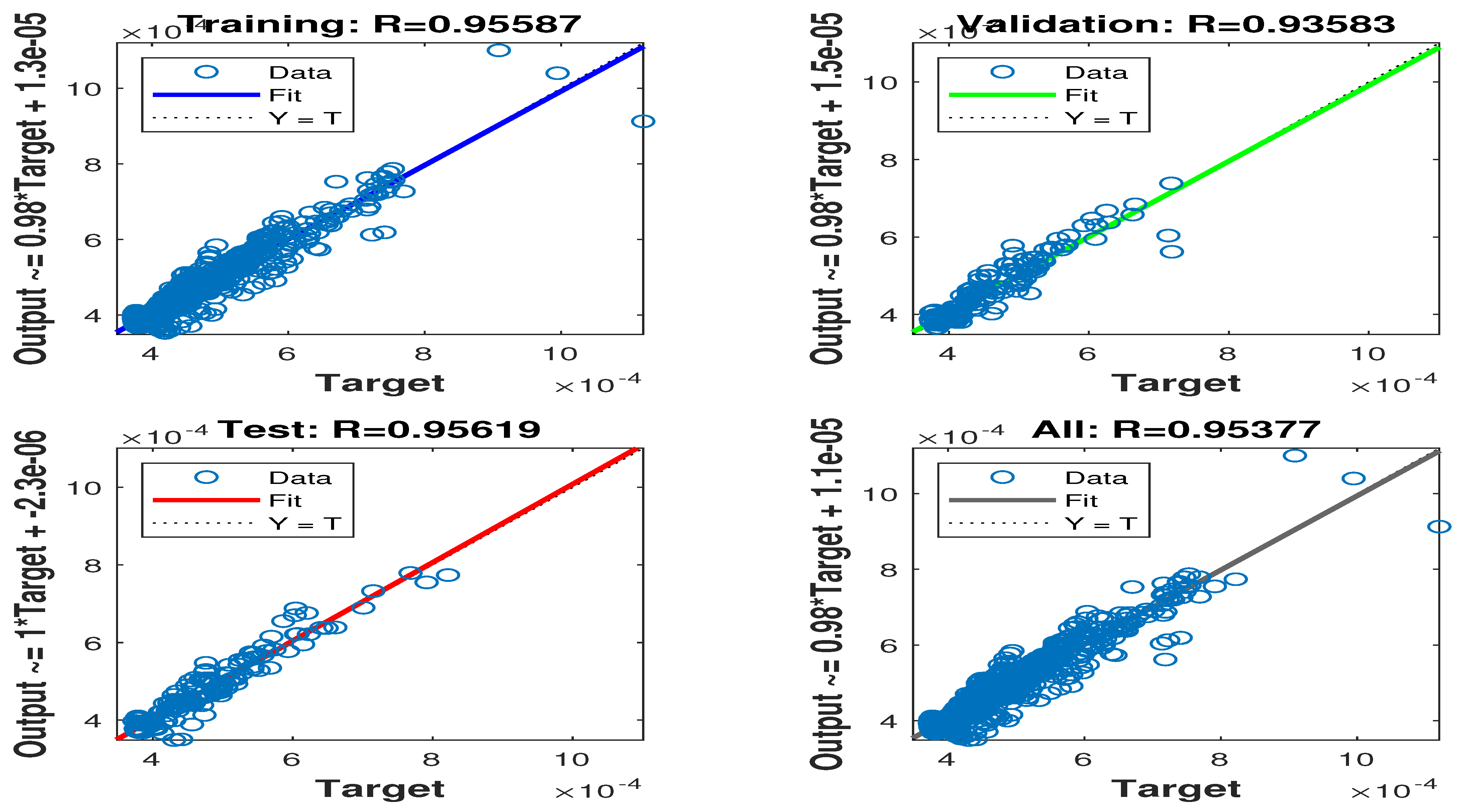
Inherent in this design is the neural network’s capacity to learn an approximation of the functional relationship between the input weights and the resultant semivariance, predicated on the provided 1000 data samples. Thus, rather than engaging in the direct computation of semivariance within the optimization process, we leverage a machine learning model to execute this task. Specifically, our aim is to utilize the neural network to approximate the objective function (semivariance) and subsequently perform a minimization procedure on this approximation to ascertain the optimal weight allocations. Fundamentally, the training of the neural network in this design entails learning a non-linear mapping function that transforms the stock weights to the corresponding semivariance value. As is visually represented in Figure 4, the attainment of a coefficient of determination (R) of 0.95 in the regression analysis conducted within the internal layers of the neural network’s learning process signifies a remarkably robust model fit. This indicates that the regression model trained within these internal layers has successfully accounted for 95 percent of the variance observed in the target variable, which is likely an intermediate feature intrinsically linked to portfolio semivariance.

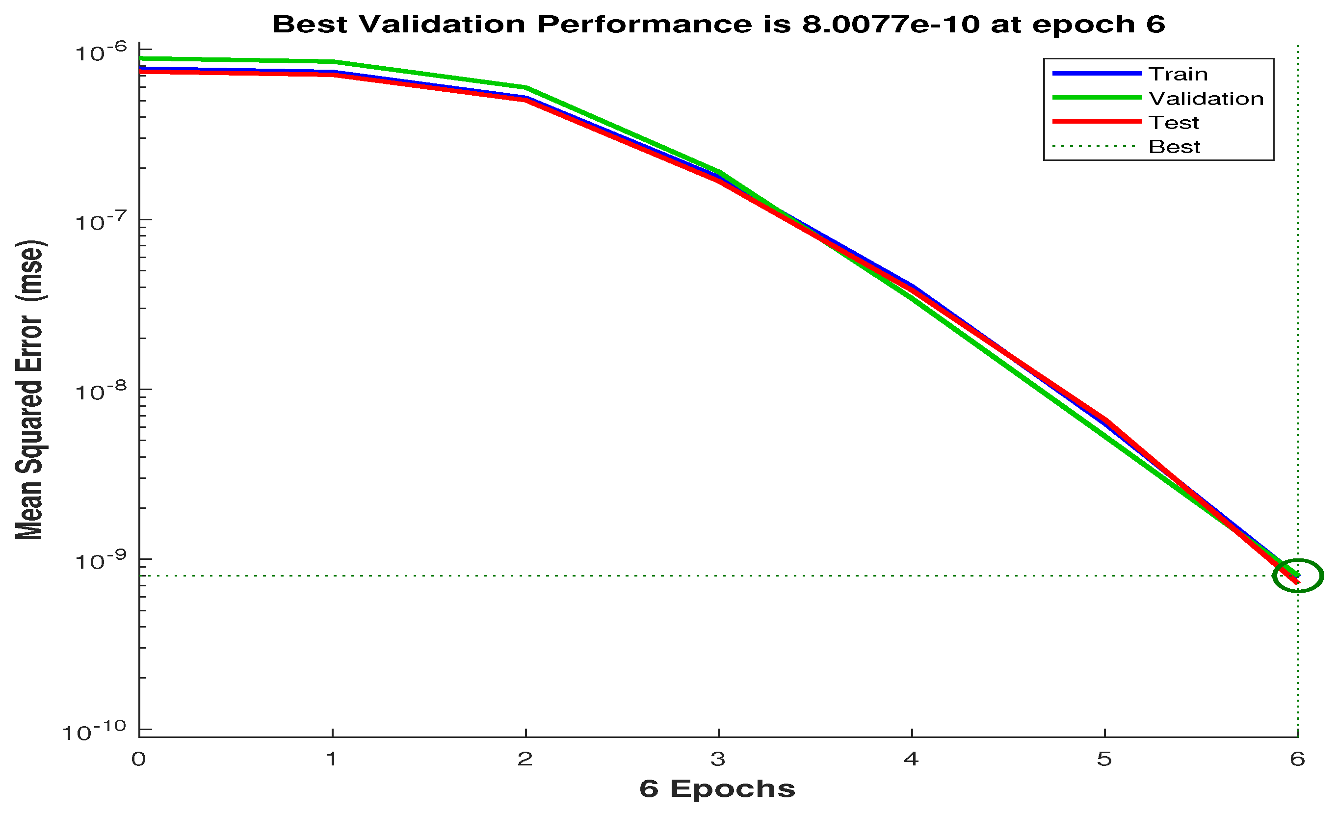
The neural network, in its preceding layers, has demonstrated a proficiency in extracting salient and pertinent features from the input data. These extracted features exhibit a strong correlative relationship with the target variable within the internal layers. The regression model (which may be a straightforward linear regression or a more complex non-linear formulation) trained on these extracted features has effectively modeled the relationship between these features and the target variable. This substantial goodness-of-fit within the internal layers underscores the considerable potential of the neural network to learn intricate data patterns and generate precise outputs, such as portfolio risk assessments. The declining trajectory of the mean squared error (MSE) throughout the training regimen constitutes a highly favorable and indispensable indicator of model performance. Figure 5 illustrates the model’s ongoing learning and performance enhancement; with each training epoch or iteration, the neural network adaptively adjusts its internal weights to bring its output predictions (portfolio semivariance) closer to the actual or target values. A lower MSE value directly corresponds to a higher degree of accuracy in the model’s predictive or generative capabilities. A consistently decreasing MSE trend signifies a continuous improvement in the model’s precision. Furthermore, a stable descent in MSE suggests that the training process is converging towards an optimal (or at least a locally optimal) solution where the prediction error is minimized. The results thus obtained underscore the promising nature of employing neural networks for portfolio optimization within the capital market. The model has exhibited a notable capacity to learn complex data relationships, and its performance has demonstrably improved over the course of its training.

Upon meticulous examination of

Table 5. Weight of the efficient stock.

Asset ID	DEA-$\mathit{\beta }$-MSV	DEA-$\mathit{\beta }$-MSV-NSGA2	DEA-$\mathit{\beta }$-MSV-SPEA2	DEA-$\mathit{\beta }$-MSV-NN
1	0.0039	0.2426	0.0499	0.3687
8	0.6255	0.4400	0.6429	0.3456
21	0.3706	0.3174	0.3072	0.2857

, it becomes evident that the neural network demonstrates precisely the behavior anticipated from a rational portfolio optimization process. The empirical observation that assets exhibiting the lowest semivariance (a measure of downside risk) and the highest returns ultimately receive the most substantial weight allocations within the optimized portfolio underscores the efficacy of the proposed methodology in synergistically integrating machine learning (specifically, the neural network for the explicit modeling of portfolio semivariance) with a robust optimization algorithm (in this instance, the interior-point method). In essence, the optimization algorithm, leveraging the risk predictions generated by the neural network as its objective function, has operated judiciously by preferentially allocating a greater weight to those assets that offer superior returns commensurate with lower levels of risk exposure. This principle constitutes the bedrock of a judicious investment strategy.

Furthermore, the proposed neural network has demonstrably acquired a robust understanding of the intricate relationship between the specific weight allocations assigned to individual stocks and the resultant overall risk profile of the composite portfolio. Consequently, the optimization algorithm has been effectively guided, through the informed outputs of the neural network, towards asset allocations predominantly comprising stocks characterized by desirable attributes, namely, a low risk and high return potential. This outcome is fundamentally congruent with established investment tenets that advocate for either the maximization of returns for a given, predetermined level of risk tolerance or, conversely, the minimization of risk exposure for a specified target level of return. The strategic allocation of a greater weight to assets exhibiting lower risk profiles coupled with higher return prospects represents a demonstrably rational investment heuristic that can significantly assist investors in the pursuit and attainment of their articulated financial objectives. A portfolio meticulously optimized according to these well-established principles is demonstrably more likely to exhibit superior performance over extended investment horizons when contrasted with portfolios constructed through either stochastic weight allocations or those predicated solely on intuitive judgments. This anticipated outperformance is directly attributable to the explicit focus on assets possessing both a substantial return potential and comparatively modest levels of risk. Conversely, the application of evolutionary algorithms and the traditional optimization method resulted in the predominant allocation of weight to the individual stock exhibiting the highest absolute return (stock # 8).

These alternative methodologies assigned comparatively minimal weight to stocks characterized by lower semivariance, a decision that consequently led to elevated levels of overall portfolio risk within the optimized portfolios, as explicitly detailed in

Table 6. Return and risk of the models.

Model	Return	Risk
DEA-$\beta$- MSV-NN	0.0026	0.0008
DEA-$\beta$- MSV-NSGA2	0.0028	0.0177
DEA-$\beta$ -MSV-SPEA2	0.0032	0.0203
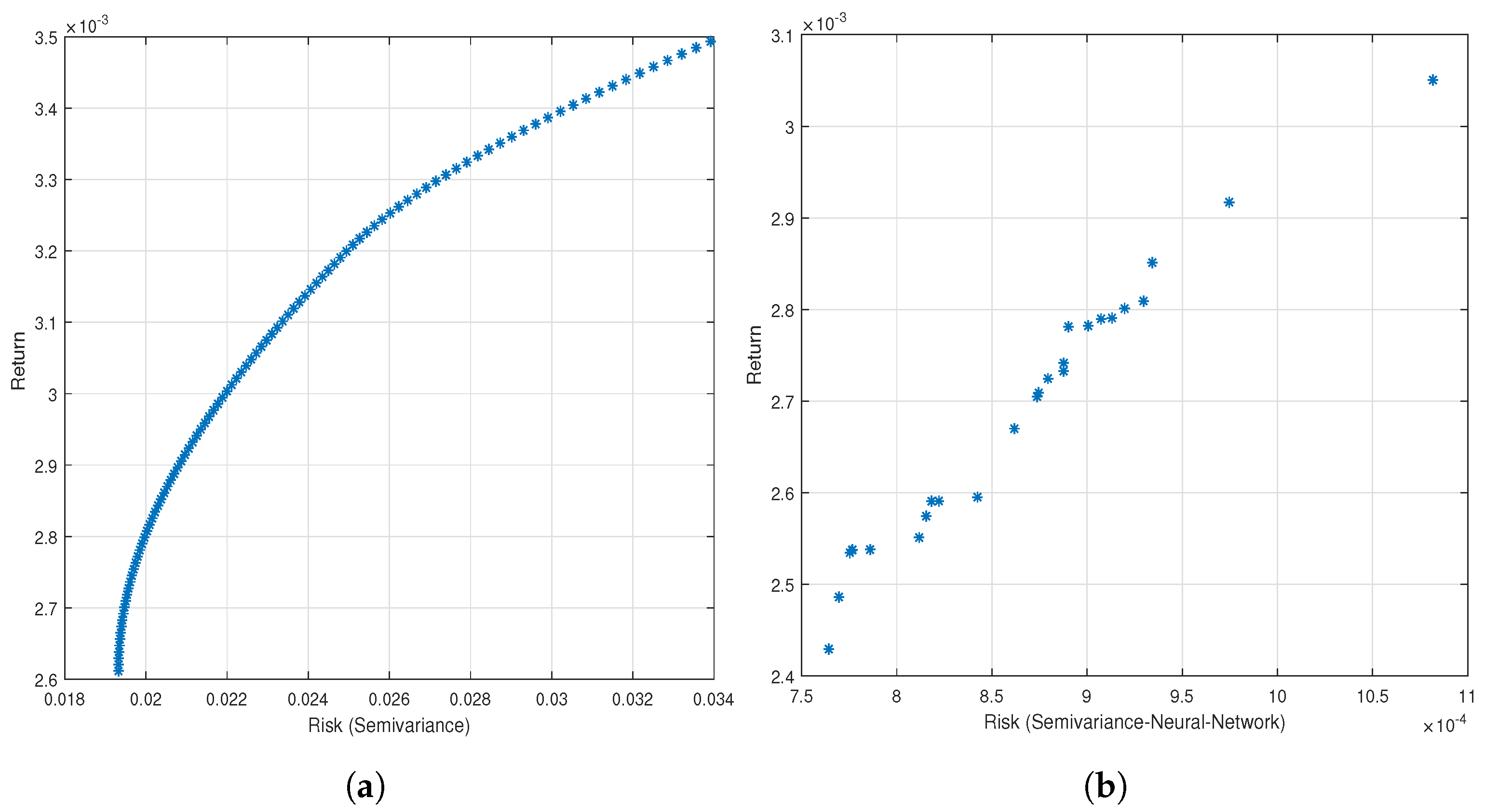
DEA-$\beta$- MSV	0.0032	0.0242

. In stark contrast, the aggregate risk associated with the portfolio constructed through the informed application of the neural network is demonstrably and significantly lower. Moreover, as visually elucidated in Figure 6 and Figure 7, the portfolios generated through the neural network approach consistently exhibit lower levels of risk exposure when directly compared to those portfolios derived from the implementation of evolutionary algorithms and the traditional method. By way of concrete illustration, for a comparable level of portfolio return approximating $0.03$, the neural network-optimized portfolio exhibits a markedly lower risk level of $0.0008$, whereas the risk levels associated with portfolios generated by the alternative methodologies are substantially higher, approximating $0.02$.

To further examine the portfolios generated by the introduced methods, their efficiency was evaluated using DEA in

Table 7. Input and output consist of risk and return of portfolios.

		Inputs		Outputs
Portfolio	NSGA2 Risk	SPEA2 Risk	NN Risk	NSGA2 Rerurn	SPEA2 Return	NN Return
1	0.019	0.0215	0.0008	0.003	0.0033	0.0026
2	0.0194	0.0204	0.0004	0.0031	0.0032	0.0017
3	0.022	0.0233	0.0007	0.0033	0.0034	0.0024
4	0.0176	0.0188	0.0007	0.0028	0.003	0.0025
5	0.0188	0.0267	0.0007	0.003	0.0035	0.0024
6	0.0232	0.0241	0.0007	0.0034	0.0034	0.0025
7	0.0177	0.026	0.0007	0.002	0.0035	0.0025
8	0.0248	0.0207	0.0007	0.0034	0.0032	0.0025
9	0.025	0.0175	0.0008	0.0034	0.0028	0.0025
10	0.0188	0.0211	0.0008	0.003	0.0032	0.0025
11	0.0177	0.0203	0.0008	0.0028	0.0032	0.0025

and

Table 8. Efficiency of portfolios.

	Efficiency
Portfolio	NSGA2	SPEA2	NN
1	0.9881	0.9593	1
2	1	0.9804	1
3	0.9387	0.912	0.9653
4	0.9956	0.9973	0.9814
5	0.9986	0.8193	0.9339
6	0.9171	0.8817	0.9742
7	0.6897	0.8413	1
8	0.858	0.9662	0.9922
9	0.8511	1	0.9561
10	0.9986	0.9479	0.9542
11	0.9655	0.9852	0.9725

. As observed, the neural network produced a greater number of efficient portfolios compared to the other two methods. The superior performance of the neural network in generating a larger number of efficient portfolios likely indicates its enhanced capability in learning the complex relationships between input variables (weights) and output variables (risk) within the capital market. The neural network may have identified non-linear and subtle patterns that the evolutionary algorithms were not readily able to discover, leading to the generation of portfolios that offer lower risk relative to the accepted return.

The second-place ranking of NSGA2 in terms of the number of efficient portfolios suggests that this evolutionary algorithm also demonstrated a respectable performance in identifying a set of pareto-optimal portfolios (trade-off between risk and return). NSGA2 is well-recognized for its efficacy in searching the solution space and identifying a set of non-dominated solutions (where no other solution is superior in all objectives). The last-place ranking of the SPEA2 algorithm in terms of the number of efficient portfolios may indicate that this algorithm, in comparison to the neural network and NSGA2, was less successful in identifying portfolios that simultaneously performed well across all efficiency criteria (DEA inputs and outputs). This could be attributed to the algorithm’s structure, parameter settings, or its search strategy within the solution space.

These results can be interpreted as corroborating evidence for the significant potential of neural networks as a powerful tool in portfolio optimization. Their ability to learn intricate patterns may render them superior in identifying optimal asset allocations that establish a more favorable equilibrium between risk and return. The results demonstrate that the selection of the optimization algorithm has a significant impact on the efficiency of the final portfolios. Depending on the characteristics of the market and the investor’s objectives, one method may outperform another. The performance of evolutionary algorithms such as NSGA2 and SPEA2 is highly dependent on the tuning of their parameters. It is plausible that with more precise parameter adjustments, their performance could be improved. These findings could provide impetus for exploring the combination of different optimization methods (such as utilizing the neural network’s output as an initial population for a genetic algorithm) to leverage the inherent strengths of each approach.

Computational Complexity

This section provides a detailed analysis of the computational resources and time required for each component of our integrated methodology. Understanding these execution times is crucial for evaluating the practical applicability and scalability of our approach, and it clearly highlights the trade-off between solution quality and computational cost.

In portfolio optimization using a neural network, where we employed a two-stage method, the neural network training time was merely 2 s (it should be noted that early stopping was employed to prevent overfitting), and the time to find optimal weights based on the predicted semivariance was 0.5 s. Cumulatively, solving this problem with the neural network took only 2.5 s. In contrast, when solving the same problem with the NSGA2 and the SPEA2 (both configured with 100 iterations (generations) and a population size of 50), finding the optimal weights required 40 and 45 s, respectively. This direct comparison clearly demonstrates the inherent trade-off between solution quality and computational cost across the different methodologies.

The most significant advantage of our neural network-based approach emerges in its extraordinary operational speed during the second stage. After the initial neural network training (which was completed at a negligible cost of 2 s), the process of finding an optimal portfolio for a specified return is remarkably fast, typically taking only milliseconds. This unparalleled speed makes our approach highly suitable for real-time portfolio adjustments or high-frequency decision-making scenarios, where the iterative and inherently slower nature of evolutionary algorithms would be prohibitive. This highlights a clear trade-off: a very low initial training cost for the neural network, but in return, a negligible operational cost for each decision.

This characteristic provides superior speed and deterministic results compared to the stochastic nature of evolutionary algorithm executions. Among the two evolutionary algorithms tested, NSGA2 demonstrated a superior performance in terms of both solution quality and computational efficiency. NSGA2 completed its optimization on average in 40 s, indicating a slight computational advantage over SPEA2, which took approximately 45 s. Consequently, our two-stage approach, which utilizes a neural network as a semivariance surrogate model, significantly enhances the speed and scalability of portfolio optimization after initial training, making it ideal for dynamic market environments.

6. Conclusions

This study introduces a novel approach to portfolio optimization by integrating the DEA model with the MSV framework. Initially, the DEA model assesses asset efficiency using semivariance and beta as risk inputs and expected return as the output. Subsequently, an optimal portfolio is constructed from the identified efficient stocks. To determine the optimal weights of these stocks within the portfolio, the MSV model is solved using both a neural network and evolutionary algorithms (NSGA2 and SPEA2). In the neural network-based optimization method, random weights are fed into the neural network, with the portfolio’s semivariance serving as the output. This output then acts as the objective function to determine the optimal asset weights. Conversely, in the evolutionary algorithm-based optimization, the MSV model is solved for the efficient stocks using the NSGA2 and SPEA2 algorithms, and their respective outcomes are compared. The findings indicate that optimizing efficient stocks with a neural network significantly reduces the portfolio risk and yields higher efficiency compared to both evolutionary algorithm-based methods. Notably, the NSGA2 algorithm outperforms SPEA2 in this context. These results suggest that neural networks are effective in discerning the inherent non-linear behavior within market data, thus offering investors a valuable tool for both forecasting and optimizing their investment portfolios. The success of the neural network in solving the semivariance model underscores its robust learning capabilities. Furthermore, the favorable performance of genetic algorithms in generating efficient portfolios opens promising avenues for future research, particularly in integrating the neural network’s objective function with these algorithms for enhanced optimization and analysis.

The findings of this research are derived from data pertaining to the Iranian automotive sector over a specific period. Consequently, the unique fluctuations of the Iranian market may have influenced the model’s performance. Therefore, the proposed model’s performance requires further testing and validation in other markets such as developed markets with different regulatory frameworks or additional emerging markets—as well as across different asset classes, including bonds, commodities, and currencies. Additionally, generalizing these results to markets experiencing lower returns, recessionary conditions, or crises requires further validation. Hence, to further develop the DEA-$\beta$-MSV framework and broaden its applicability in more intricate market scenarios, several promising avenues for future research exist. In illiquid and noisy data markets (e.g., small-cap stocks), robust optimization can be employed to effectively manage the inherent uncertainties in return and risk estimations.

It will be crucial to integrate liquidity constraints and transaction cost models into the optimization problem, while also leveraging robust DEA models for more reliable asset filtering in such volatile conditions. For bond portfolios, the concept of downside risk can be redefined using yield spread semivariance, necessitating re-training the ANN on bond-specific data and incorporating bond-specific constraints (like duration and credit rating) into the optimization model. Furthermore, DEA inputs and outputs will require updates to accurately assess the bond efficiency. Finally, to ensure the framework’s adaptability to dynamic market conditions (e.g., during crises), implementing a rolling-window strategy is vital. This involves periodic updates of the DEA, re-training or fine-tuning the ANN, and re-executing the optimization process. Moreover, regime-switching models can be utilized to dynamically adjust parameters and strategies in response to evolving market states.

References

1. Markowitz, H.M. Portfolio Selection: Efficient Diversification of Investments; John Wiley: Hoboken, NJ, USA, 1959. [Google Scholar]
2. Markowitz, H.; Todd, P.; Xu, G.; Yamane, Y. Computation of mean-semivariance efficient sets by the critical line algorithm. Ann. Oper. Res. 1993, 45, 307–317. [Google Scholar] [CrossRef]
3. Huang, X. Mean-semivariance models for fuzzy portfolio selection. J. Comput. Appl. Math. 2008, 217, 1–8. [Google Scholar] [CrossRef]
4. Tsai, M.F.; Wang, C.J. Post-modern portfolio theory for information retrieval. Procedia Comput. Sci. 2012, 13, 80–85. [Google Scholar] [CrossRef]
5. Qin, Z.; Wang, D.Z.; Li, X. Mean-semivariance models for portfolio optimization problem with mixed uncertainty of fuzziness and randomness. Int. J. Uncertain. Fuzziness Knowl.-Based Syst. 2013, 21 (Suppl. S1), 127–139. [Google Scholar] [CrossRef]
6. Gökgöz, F.; Atmaca, M.E. Portfolio optimization under lower partial moments in emerging electricity markets: Evidence from Turkey. Renew. Sustain. Energy Rev. 2017, 67, 437–449. [Google Scholar] [CrossRef]
7. Chen, W.; Li, D.; Lu, S.; Liu, W. Multi-period mean–semivariance portfolio optimization based on uncertain measure. Soft Comput. 2019, 23, 6231–6247. [Google Scholar] [CrossRef]
8. Hamdi, A.; Khodamoradi, T.; Salahi, M. A penalty decomposition algorithm for the extended mean–variance–CVaR portfolio optimization problem. Discret. Math. Algorithms Appl. 2023, 16, 2350021. [Google Scholar] [CrossRef]
9. Chochola, O.; Hušková, M.; Prášková, Z.; Steinebach, J.G. Robust monitoring of CAPM portfolio betas. J. Multivar. Anal. 2013, 115, 374–395. [Google Scholar] [CrossRef]
10. Chochola, O.; Hušková, M.; Prášková, Z.; Steinebach, J.G. Robust monitoring of CAPM portfolio betas II. J. Multivar. Anal. 2014, 132, 58–81. [Google Scholar] [CrossRef]
11. Hur, S.K.; Chung, C.Y. Revisiting CAPM betas in an incomplete market: Evidence from the Korean stock market. Financ. Res. Lett. 2017, 21, 241–248. [Google Scholar] [CrossRef]
12. Cenesizoglu, T.; Reeves, J.J. CAPM, components of beta and the cross section of expected returns. J. Empir. Financ. 2018, 49, 223–246. [Google Scholar] [CrossRef]
13. Charnes, A.; Cooper, W.W.; Rhodes, E. Measuring the efficiency of decision making units. Eur. J. Oper. Res. 1978, 2, 429–444. [Google Scholar] [CrossRef]
14. Morey, M.R.; Morey, R.C. Mutual fund performance appraisals: A multi-horizon perspective with endogenous benchmarking. Omega 1999, 27, 241–258. [Google Scholar] [CrossRef]
15. Lamb, J.D.; Tee, K.H. Data envelopment analysis models of investment funds. Eur. J. Oper. Res. 2012, 216, 687–696. [Google Scholar] [CrossRef]
16. Branda, M. Diversification-consistent data envelopment analysis with general deviation measures. Eur. J. Oper. Res. 2013, 226, 626–635. [Google Scholar] [CrossRef]
17. Xiao, H.; Ren, T.; Zhou, Z.; Liu, W. Parameter uncertainty in estimation of portfolio efficiency: Evidence from an interval diversification-consistent DEA approach. Omega 2021, 103, 102357. [Google Scholar] [CrossRef]
18. Zhou, Z.; Gao, M.; Xiao, H.; Wang, R.; Liu, W. Big data and portfolio optimization: A novel approach integrating DEA with multiple data sources. Omega 2021, 104, 102479. [Google Scholar] [CrossRef]
19. Hamdi, A.; Karimi, A.; Mehrdoust, F.; Belhaouari, S.B. Portfolio Selection Problem Using CVaR Risk Measures Equipped with DEA, PSO, and ICA Algorithms. Mathematics 2022, 10, 2808. [Google Scholar] [CrossRef]
20. Branda, M. Reformulations of input–output oriented DEA tests with diversification. Oper. Res. Lett. 2013, 41, 516–520. [Google Scholar] [CrossRef]
21. Sharpe, W.F. A simplified model for portfolio analysis. Manag. Sci. 1963, 9, 277–293. [Google Scholar] [CrossRef]
22. Carlsson, C.; Korhonen, P. A parametric approach to fuzzy linear programming. Fuzzy Sets Syst. 1986, 20, 17–30. [Google Scholar] [CrossRef]
23. Milgrom, P.; Segal, I. Envelope theorems for arbitrary choice sets. Econometrica 2002, 70, 583–601. [Google Scholar] [CrossRef]
24. Jin, H.; Markowitz, H.; Zhou, X.Y. A note on semivariance. Mathematical Finance. Int. J. Math. Stat. Financ. Econ. 2006, 16, 53–61. [Google Scholar]
Figure 1. Feedforward neural network.
Algorithms 18 00384 g001
Figure 2. Analyzed automotive market. (a) Normality test of price index. (b) Distribution of price index values with a long right tail.
Algorithms 18 00384 g002
Figure 3. The risks and return of the statistical sample. (a) Beta of any stock. (b) Semivariance of any stock. (c) Expected return of any stock.
Algorithms 18 00384 g003
Figure 4. Feedforward neural network learning regression.
Algorithms 18 00384 g004
Figure 5. Performance of feedforward neural networks.
Algorithms 18 00384 g005
Figure 6. Efficient frontier. (a) Frontiers of MSV model. (b) Frontiers of DEA- β -MSV-Neural Network model.
Algorithms 18 00384 g006
Figure 7. Efficient frontier. (a) Frontiers of DEA- β -MSV-NSGA2 model. (b) Frontiers of DEA- β -MSV-SPEA2 model.
Algorithms 18 00384 g007