An RMSprop-Incorporated Latent Factorization of Tensor Model for Random Missing Data Imputation in Structural Health Monitoring

Abstract

In structural health monitoring (SHM), ensuring data completeness is critical for enhancing the accuracy and reliability of structural condition assessments. SHM data are prone to random missing values due to signal interference or connectivity issues, making precise data imputation essential. A latent factorization of tensor (LFT)-based method has proven effective for such problems, with optimization typically achieved via stochastic gradient descent (SGD). However, SGD-based LFT models and other imputation methods exhibit significant sensitivity to learning rates and slow tail-end convergence. To address these limitations, this study proposes an RMSprop-incorporated latent factorization of tensor (RLFT) model, which integrates an adaptive learning rate mechanism to dynamically adjust step sizes based on gradient magnitudes. Experimental validation on a scaled bridge accelerometer dataset demonstrates that RLFT achieves faster convergence and higher imputation accuracy compared to state-of-the-art models including SGD-based LFT and the long short-term memory (LSTM) network, with improvements of at least 10% in both imputation accuracy and convergence rate, offering a more efficient and reliable solution for missing data handling in SHM.

1. Introduction

In recent decades, the continuous development of civil infrastructure has led to the widespread deployment of structural health monitoring (SHM) systems for real-time performance assessments. These systems continuously collect multi-modal data (e.g., vibrations, strains, and displacements) through sensors, forming the basis for damage detection and condition evaluation. However, factors such as improper installation, environmental noise, and extreme weather introduce anomalous data, significantly compromising monitoring reliability. Among these anomalies, data loss is the most prevalent. Specifically, in field applications, random missing data caused by signal interference, poor sensor connectivity, or transmission failures pose critical challenges [1,2]. Such data incompleteness not only adversely impacts downstream tasks like damage identification and state assessment but also degrades overall SHM system efficacy, making SHM data imputation a fundamentally challenging problem.

To address these challenges, multiple imputation methods have been proposed [3,4,5]. Early-stage matrix imputation approaches, such as alternating least squares (ALS), demonstrate certain advantages in handling high-dimensional incomplete (HDI) data by leveraging low-rank matrix assumptions for missing value reconstruction [6]. However, ALS exhibits limited imputation accuracy for non-low-rank structured data and high sensitivity to initialization, failing to deliver stable high-precision results. These limitations become particularly pronounced when processing temporally complex datasets.

To overcome ALS limitations, convolutional neural networks (CNNs) have been introduced for data imputation tasks. CNNs automatically learn spatial features through convolutional layers, demonstrating strong nonlinear modeling capabilities to capture complex patterns and improve imputation accuracy [7,8]. However, CNNs require highly structured spatial data and fail to fully exploit temporal dependencies when processing time-series data.

To address the CNN’s limitations in temporal data processing, long short-term memory (LSTM)-based imputation algorithms were proposed. As a specialized recurrent neural network, LSTM effectively captures long-term dependencies in time-series data through memory cells and gating mechanisms, making it particularly suitable for time-dependent SHM data. This enables more accurate missing data reconstruction by leveraging temporal patterns [9,10]. Although LSTMs excel at temporal modeling, their training complexity and susceptibility to overfitting remain challenges. Consequently, deep learning methods often struggle to fully characterize the inherent spatiotemporal coupling features in bridge SHM data [11].

Building upon these developments, the stochastic gradient descent (SGD)-based latent factorization of tensor (LFT) model was proposed [12,13,14,15]. This approach integrates tensor decomposition with SGD optimization to effectively handle multi-dimensional complex data relationships while maintaining scalability for large-scale dataset training. Compared to ALS, CNN, and LSTM, the LFT model demonstrates superior performance when processing high-dimensional, sparse, and structurally complex data. Chen et al. [16] present a momentum-incorporated biased non-negative and adaptive LFT model, which shows higher computational efficiency and missing link prediction accuracy in efficient representation learning of dynamic weighted directed networks than existing advanced models. However, the SGD-based LFT model suffers from learning rate sensitivity and slow tail-end convergence, which impair training stability and convergence speed. Additionally, its demanding hyperparameter tuning requirements limit practical usability and operational robustness.

To address these challenges, this paper proposes an RMSprop-incorporated latent factorization of tensor (RLFT) model, with the primary research focus on incorporating an adaptive learning rate mechanism into the SGD training process. Specifically, the RLFT model enhances the baseline LFT framework by integrating the RMSprop algorithm, which employs exponential moving averages of squared gradients to dynamically adjust learning rates. This adaptive mechanism effectively suppresses gradient fluctuations and accommodates sparse gradients, thereby optimizing the convergence path for smoother and more efficient training. The proposed approach not only maintains data imputation accuracy but also significantly improves the convergence rate. The key contributions include the following:

• The incorporation of the RLFT optimization model for SHM data imputation, enabling rapid convergence with properly tuned hyperparameters;
• A systematic analysis of missing rate impacts on model performance, with comprehensive RLFT algorithm design and analysis to guide engineering applications.

The paper is organized as follows: Section 2 presents preliminary concepts. Section 3 details the RLFT model. Section 4 demonstrates the experimental results and analysis. Section 5 concludes the work.

2. Preliminaries

This section presents the fundamental notations, problem formulation, and methodology concerning the HID tensor in our study.

2.1. Symbol Appointment

SHM data typically constitute HDI tensors with inherent spatiotemporal characteristics [17,18]. When utilizing such tensors as primary inputs for structural state analysis and data imputation, the target tensor contains numerous unknown elements representing missing measurements. This study specifically examines model performance under varying missing rates.

Table 1. Symbols used and their descriptions.

Symbol	Description
Y	A time point–location–working condition tensor.
T, L, W	LF matrices for time points, locations and working conditions.
I, J, K	Sets of time points, locations, and working conditions.
yijk	A single element in Y.
$\widehat{\mathbf{Y}}$	Low-rank approximation to Y based on T, L, and W.
${\widehat{y}}_{ijk}$	A single element in $\widehat{\mathbf{Y}}$.
R	Rank of $\widehat{\mathbf{Y}}$.
tr,lr,wr	LF vectors for the rth rank-one tensor in $\widehat{\mathbf{Y}}$.
tir, ljr, wkr	Single LF in T, L, and W.
ℝ	Real number domain.
Λ	Known dataset of Y.
Γ	Unknown dataset of Y.

summarizes the mathematical notations and their definitions for tensor-based latent factorization.

2.2. Problem Formulation

A multi-dimensional representation is constructed for a structural state in SHM data by modeling these relationships as a third-order tensor, capturing high-dimensional features across various time points, locations, and working conditions. For an incomplete tensor Y, each element y_ijk represents the acceleration measurement recorded at the jth sensor location and ith time point under the kth working condition.

Let Λ and Γ denote the known and unknown datasets of Y, respectively. The canonical polyadic (CP) tensor-based latent factor (LF) decomposition method [19,20,21,22,23,24,25,26,27] constructs an approximation $\widehat{\mathbf{Y}}$ of the original tensor Y, as shown in Equation (1) [19]:

$$\widehat{\mathbf{Y}}={\displaystyle \sum _{r=1}^R{\mathbf{X}}_{\mathit{r}}}$$

(1)

where each component tensor X_r is defined as follows:

The tensor Y is decomposed into R rank-one tensors X₁, X₂, …, X_R. Each rank-one tensor X_r∈ ℝ^{|I|×|J|×|K|} can be expressed as the outer product of three LF vectors t_r, l_r, and w_r with lengths |I|, |J|, and |K|, respectively, as shown in Equation (2) [19]:

$${\mathbf{X}}_{\mathit{r}}={\mathit{t}}_{\mathit{r}}\circ {\mathit{l}}_{\mathit{r}}\circ {\mathit{w}}_{\mathit{r}}$$

(2)

Each element in X_r is given by Equation (3) [20]:

$$a_{ijk}=t_{ir}{l}_{jr}{w}_{kr}$$

(3)

The rth LF vectors from matrices T, L, and W collectively form the rth rank-one tensor X_r, yielding the approximation $\widehat{\mathbf{Y}}$. Each element ${\widehat{y}}_{ijk}$ in $\widehat{\mathbf{Y}}$ is computed as Equation (4) [20]:

$${\widehat{y}}_{ijk}={\displaystyle \sum _{r=1}^R{l}_{it}{t}_{jr}{s}_{kr}}$$

(4)

Considering only the data in Λ, the discrepancy between the corresponding elements of Y and $\widehat{\mathbf{Y}}$ is measured using the Euclidean distance metric. To prevent overfitting, regularization terms are incorporated, yielding the objective loss function (Equation (5)) [21]:

$$\epsilon ={\displaystyle \sum _{y_{ijk}\in \Lambda }({(y_{ijk}-{\widehat{y}}_{ijk})}^2+{\lambda }_t{\displaystyle \sum _{r=1}^R{t}_{ir}^2+}{\lambda }_l{\displaystyle \sum _{r=1}^R{l}_{jr}^2+}{\lambda }_w{\displaystyle \sum _{r=1}^R{w}_{kr}^2})}$$

(5)

where λ_t, λ_l, and λ_w denote the regularization coefficients for the latent feature matrices T, L, and W, respectively.

2.3. RMSprop Method

The RMSprop method dynamically adjusts learning rates by combining adaptive learning rate mechanisms with accumulated gradient squares, thereby accelerating model training. Specifically, it employs exponentially weighted moving averages to accumulate squared gradients, incorporating historical gradient magnitudes during parameter updates. This accumulation effectively mitigates gradient oscillations, particularly for sparse gradients or non-stationary objectives, enabling self-adaptive learning rate adjustment. During iterative training, RMSprop applies bias correction to the accumulated gradient squares to ensure accurate initial estimates, ultimately computing parameter-specific adaptive learning rates to accelerate convergence and enhance optimization stability. For a given objective function J(θ), the parameter θ is updated with adaptive learning rates, as shown in Equation (6) [12]:

$$\begin{array}{l}{A}_0=0;A_s=\gamma A_{s-1}+(1-\gamma ){(\nabla J({\theta }_{s-1},o_s))}^2\\ {\theta }_s={\theta }_{s-1}-(\eta \cdot \nabla J({\theta }_{s-1},o_s)/\sqrt{A_s+\delta })\end{array}$$

(6)

where A₀ denotes the initial value of the accumulated squared gradients, while A_s−1 and A_s represent the accumulated squared gradients at time steps s − 1 and s, respectively. The decay rate γ controls the weighting of historical information. The variables θ_s−1 and θ_s correspond to the parameter states at iterations s − 1 and s, and o_s indicates the training instance encountered during the sth update. The base learning rate η and a small constant δ (to prevent division by zero) complete the parameter set.

3. RMSprop SGD-Based LFT Model

This section presents our proposed RLFT model that enhances traditional SGD-based LFT through adaptive learning rate optimization. The following subsections detail the baseline implementation (Section 3.1), our improved RLFT model (Section 3.2), and algorithmic analysis (Section 3.3).

3.1. Standard SGD-Based LFT Model

In LF analysis, the SGD-based LFT stands out for its straightforward operation and computationally efficient performance. This algorithm calculates the gradient for each training sample and adjusts the parameters in the opposite direction of this gradient, thereby continuously optimizing and progressively reducing the value of the target loss function (5). With SGD, the objective loss function is minimized, as shown in Equation (7) [22]:

$$\begin{array}{l}\underset{T,L,W}{\arg \min }\epsilon (T,L,W)\stackrel{SGD}{\Rightarrow }\forall i\in I,j\in J,k\in K,r\in \{1,2,\dots ,R\}:\\ t_{ir}^s\leftarrow t_{ir}^{s-1}-{\eta }_{ir}{\displaystyle \frac{\partial {\epsilon }_{ijk}^{s-1}}{\partial t_{ir}^{s-1}}},l_{jr}^s\leftarrow l_{jr}^{s-1}-{\eta }_{jr}{\displaystyle \frac{\partial {\epsilon }_{ijk}^{s-1}}{\partial l_{jr}^{s-1}}},w_{kr}^s\leftarrow w_{kr}^{s-1}-{\eta }_{kr}{\displaystyle \frac{\partial {\epsilon }_{ijk}^{s-1}}{\partial w_{kr}^{s-1}}}\end{array}$$

(7)

where ${\epsilon }_{ijk}={(y_{ijk}-{\widehat{y}}_{ijk})}^2+{\lambda }_t{\displaystyle \sum _{r=1}^R{t}_{ir}^2+}{\lambda }_l{\displaystyle \sum _{r=1}^R{l}_{jr}^2+}{\lambda }_w{\displaystyle \sum _{r=1}^R{w}_{kr}^2}$ represents the instantaneous loss corresponding to an individual training instance y_ijk ∈ Λ, s denotes the sth update point, and η_ir, η_jr, and η_kr represent the learning rates for t_ir, l_jr, and w_kr, respectively. The gradient formula is given by Equation (8) [22]:

$$\begin{array}{l}{\displaystyle \frac{\partial {\epsilon }_{ijk}^{s-1}}{\partial t_{ir}^{s-1}}}={\lambda }_t{t}_{ir}^{s-1}-l_{jr}^{s-1}{w}_{kr}^{s-1}(y_{ijk}-{\widehat{y}}_{ijk}^{s-1})\\ {\displaystyle \frac{\partial {\epsilon }_{ijk}^{s-1}}{\partial l_{jr}^{s-1}}}={\lambda }_l{l}_{jr}^{s-1}-t_{ir}^{s-1}{w}_{kr}^{s-1}(y_{ijk}-{\widehat{y}}_{ijk}^{s-1})\\ {\displaystyle \frac{\partial {\epsilon }_{ijk}^{s-1}}{\partial w_{kr}^{s-1}}}={\lambda }_w{w}_{kr}^{s-1}-t_{ir}^{s-1}{l}_{jr}^{s-1}(y_{ijk}-{\widehat{y}}_{ijk}^{s-1})\end{array}$$

(8)

Substituting Formula (7) into Formula (6) yields Equation (9) [22]:

$$\begin{array}{l}\underset{T,L,W}{\arg \min }\epsilon (T,L,W)\stackrel{SGD}{\Rightarrow }\forall i\in I,j\in J,k\in K,r\in \{1,2,\dots ,R\}:\\ t_{ir}^s\leftarrow t_{ir}^{s-1}-{\eta }_{ir}({\lambda }_t{t}_{ir}^{s-1}-l_{jr}^{s-1}{w}_{kr}^{s-1}(y_{ijk}-{\widehat{y}}_{ijk}^{s-1}))\\ l_{jr}^s\leftarrow l_{jr}^{s-1}-{\eta }_{jr}({\lambda }_l{l}_{jr}^{s-1}-t_{ir}^{s-1}{w}_{kr}^{s-1}(y_{ijk}-{\widehat{y}}_{ijk}^{s-1}))\\ w_{kr}^s\leftarrow w_{kr}^{s-1}-{\eta }_{kr}({\lambda }_w{w}_{kr}^{s-1}-t_{ir}^{s-1}{l}_{jr}^{s-1}(y_{ijk}-{\widehat{y}}_{ijk}^{s-1}))\end{array}$$

(9)

3.2. RLFT Model

In the SGD-based LFT model, if the objective function’s surface exhibits complex topography (such as elongated valleys), the gradient direction may deviate from the optimal path, leading to slow convergence or even oscillations. The RMSprop algorithm addresses this by employing exponentially weighted moving averages of squared gradients to dynamically adapt the learning rate. This approach mitigates gradient fluctuations and accommodates sparse gradients, thereby optimizing the path toward more stable and efficient convergence. As illustrated in Figure 1, RMSprop demonstrates a more direct trajectory toward the optimal solution, achieving faster convergence with reduced oscillations. Therefore, adopting the RMSprop algorithm is essential for enhancing model training efficiency in complex optimization problems.

When integrating the adaptive learning rate method (i.e., the RMSprop algorithm) into the SGD-based LFT model, it is also necessary to update the decision parameters for each training instance during every iteration. According to Formula (6), the update rules for t_ir, l_jr, and w_kr can be derived by following Equations (10)–(12) [23]:

The update of t_ir is as follows:

$$\begin{array}{l}{A}_{t_{ir}}^0=0;A_{t_{ir}}^s=\gamma A_{t_{ir}}^{s-1}+(1-\gamma ){({\displaystyle \frac{\partial {\epsilon }_{ijk}^{s-1}}{\partial t_{ir}^{s-1}}})}^2\\ t_{ir}^s=t_{ir}^{s-1}-{\displaystyle \frac{{\eta }_{ir}}{\sqrt{A_{t_{ir}}^s+\delta }}}\cdot {\displaystyle \frac{\partial {\epsilon }_{ijk}^{s-1}}{\partial t_{ir}^{s-1}}}\end{array}$$

(10)

The update of l_jr is as follows:

$$\begin{array}{l}{A}_{l_{jr}}^0=0;A_{l_{jr}}^s=\gamma A_{l_{jr}}^{s-1}+(1-\gamma ){({\displaystyle \frac{\partial {\epsilon }_{ijk}^{s-1}}{\partial l_{jr}^{s-1}}})}^2\\ l_{jr}^s=l_{jr}^{s-1}-{\displaystyle \frac{{\eta }_{jr}}{\sqrt{A_{l_{jr}}^s+\delta }}}\cdot {\displaystyle \frac{\partial {\epsilon }_{ijk}^{s-1}}{\partial l_{jr}^{s-1}}}\end{array}$$

(11)

The update of w_kr is as follows:

$$\begin{array}{l}{A}_{w_{kr}}^0=0;A_{w_{kr}}^s=\gamma A_{w_{kr}}^{s-1}+(1-\gamma ){({\displaystyle \frac{\partial {\epsilon }_{ijk}^{s-1}}{\partial w_{kr}^{s-1}}})}^2\\ w_{kr}^s=w_{kr}^{s-1}-{\displaystyle \frac{{\eta }_{kr}}{\sqrt{A_{w_{kr}}^s+\delta }}}\cdot {\displaystyle \frac{\partial {\epsilon }_{ijk}^{s-1}}{\partial w_{kr}^{s-1}}}\end{array}$$

(12)

By combining Formulas (10)–(12) with Formula (8), the objective loss function is minimized, as shown in Equation (13) [23]:

$$\begin{array}{l}\underset{T,L,W}{\arg \min }\epsilon (T,L,W)\stackrel{RLFT}{\Rightarrow }\forall i\in I,j\in J,k\in K,r\in \{1,2,\dots ,R\}:\\ \left\{\begin{array}{l}{A}_{t_{ir}}^0=0;A_{t_{ir}}^s=\gamma A_{t_{ir}}^{s-1}+(1-\gamma ){({\lambda }_t{t}_{ir}^{s-1}-l_{jr}^{s-1}{w}_{kr}^{s-1}(y_{ijk}-{\widehat{y}}_{ijk}^{s-1}))}^2\\ t_{ir}^s\leftarrow t_{ir}^{s-1}-{\displaystyle \frac{{\eta }_{ir}}{\sqrt{A_{t_{ir}}^s+\delta }}}\cdot ({\lambda }_t{t}_{ir}^{s-1}-l_{jr}^{s-1}{w}_{kr}^{s-1}(y_{ijk}-{\widehat{y}}_{ijk}^{s-1}))\\ A_{l_{jr}}^0=0;A_{l_{jr}}^s=\gamma A_{l_{jr}}^{s-1}+(1-\gamma ){({\lambda }_l{l}_{jr}^{s-1}-t_{ir}^{s-1}{w}_{kr}^{s-1}(y_{ijk}-{\widehat{y}}_{ijk}^{s-1}))}^2\\ l_{jr}^s\leftarrow l_{jr}^{s-1}-{\displaystyle \frac{{\eta }_{jr}}{\sqrt{A_{l_{jr}}^s+\delta }}}\cdot ({\lambda }_l{l}_{jr}^{s-1}-t_{ir}^{s-1}{w}_{kr}^{s-1}(y_{ijk}-{\widehat{y}}_{ijk}^{s-1}))\\ A_{w_{kr}}^0=0;A_{w_{kr}}^s=\gamma A_{w_{kr}}^{s-1}+(1-\gamma ){({\lambda }_w{w}_{kr}^{s-1}-t_{ir}^{s-1}{l}_{jr}^{s-1}(y_{ijk}-{\widehat{y}}_{ijk}^{s-1}))}^2\\ w_{kr}^s\leftarrow w_{kr}^{s-1}-{\displaystyle \frac{{\eta }_{kr}}{\sqrt{A_{w_{kr}}^s+\delta }}}\cdot ({\lambda }_w{w}_{kr}^{s-1}-t_{ir}^{s-1}{l}_{jr}^{s-1}(y_{ijk}-{\widehat{y}}_{ijk}^{s-1}))\end{array}\right.\end{array}$$

(13)

3.3. Algorithm Design and Analysis

To elucidate the operational principles of the RLFT model, the workflow of the RLFT algorithm is summarized as follows:

According to Algorithm 1, the computational complexity of the RLFT algorithm is characterized, as shown in Equation (14) [24]:

$$C=\Theta (2\times (\left|I\right|+\left|J\right|+\left|K\right|\times R)+N\times |\Lambda |\times 2R)\approx \Theta (N\times |\Lambda |\times R)$$

(14)

Regarding its storage complexity, this is primarily determined by (a) the known dataset Λ, (b) three LF matrices, and (c) three RMSprop correlation matrices. The storage complexity of the RLFT algorithm is formalized below using Equation (15) [24]:

$$S=\Theta ((\left|I\right|+\left|J\right|+\left|K\right|)\times R+|\Lambda |)+(|I|+|J|+|K|)\times R\approx \Theta ((\left|I\right|+\left|J\right|+\left|K\right|)\times R+|\Lambda |)$$

(15)

All the above complexity calculations disregard constant factors and lower-order terms. The above computational analysis demonstrates that the RLFT model achieves high efficiency in both computation and storage.

Algorithm 1. RLFT Algorithm
Operation	Cost
Input: Λ, R, λt, λl, λw, ηir, ηjr, ηkr, γ, δ, and iterations	-
Initializing the latent factor matrix: T, L, and W	Θ((|I| + |J| + |K|)×R)
Initializing the RMSprop correlation matrix: At, Al, and Aw = 0	Θ((|I| + |J| + |K|)×R)
for iteration = 1 to iterations (Maximum number of iterations N)	×N
for each yijk ∈ Λ	×|Λ|
${\widehat{y}}_{ijk}={\displaystyle {\sum }_{r=1}^R{t}_{ir}^{s-1}{l}_{jr}^{s-1}{w}_{kr}^{s-1}},err=y_{ijk}-{\widehat{y}}_{ijk}$	Θ(R)
for r = 1 to R do	×R
$\begin{array}{l}{A}_{t_{ir}}^s=\gamma A_{t_{ir}}^{s-1}+(1-\gamma ){({\lambda }_t{t}_{ir}^{s-1}-l_{jr}^{s-1}{w}_{kr}^{s-1}(y_{ijk}-{\widehat{y}}_{ijk}^{s-1}))}^2\\ t_{ir}^s\leftarrow t_{ir}^{s-1}-{\displaystyle \frac{{\eta }_{ir}}{\sqrt{A_{t_{ir}}^s+\delta }}}\cdot ({\lambda }_t{t}_{ir}^{s-1}-l_{jr}^{s-1}{w}_{kr}^{s-1}(y_{ijk}-{\widehat{y}}_{ijk}^{s-1}))\\ A_{l_{jr}}^s=\gamma A_{l_{jr}}^{s-1}+(1-\gamma ){({\lambda }_l{l}_{jr}^{s-1}-t_{ir}^{s-1}{w}_{kr}^{s-1}(y_{ijk}-{\widehat{y}}_{ijk}^{s-1}))}^2\\ l_{jr}^s\leftarrow l_{jr}^{s-1}-{\displaystyle \frac{{\eta }_{jr}}{\sqrt{A_{l_{jr}}^s+\delta }}}\cdot ({\lambda }_l{l}_{jr}^{s-1}-t_{ir}^{s-1}{w}_{kr}^{s-1}(y_{ijk}-{\widehat{y}}_{ijk}^{s-1}))\\ A_{w_{kr}}^s=\gamma A_{w_{kr}}^{s-1}+(1-\gamma ){({\lambda }_w{w}_{kr}^{s-1}-t_{ir}^{s-1}{l}_{jr}^{s-1}(y_{ijk}-{\widehat{y}}_{ijk}^{s-1}))}^2\\ w_{kr}^s\leftarrow w_{kr}^{s-1}-{\displaystyle \frac{{\eta }_{kr}}{\sqrt{A_{w_{kr}}^s+\delta }}}\cdot ({\lambda }_w{w}_{kr}^{s-1}-t_{ir}^{s-1}{l}_{jr}^{s-1}(y_{ijk}-{\widehat{y}}_{ijk}^{s-1}))\end{array}$	Θ(1) × 6
end for	-
end for	-
end while	-
Output LF matrix: T, L, and W	-

4. Experimental Results and Analysis

This section systematically evaluates the proposed RLFT model through comprehensive experiments. We first describe the experimental setup including datasets, evaluation metrics, and implementation details (Section 4.1), then present comparative results with state-of-the-art methods (Section 4.2). The analysis validates RLFT’s advantages in both accuracy and computational efficiency.

4.1. General Settings

The experimental configuration is organized into three components: (1) benchmark datasets for performance validation, (2) quantitative metrics for objective assessments, and (3) implementation parameters ensuring reproducible results. This standardized setup guarantees a fair comparison across all evaluated methods.

4.1.1. Datasets

To comprehensively evaluate the performance of the RLFT model, we conducted experiments using the Yunnan Hechonggou scaled bridge model dataset. This dataset records acceleration vibration signals from a 1:20 scale model of the Heichonggou Bridge, featuring high fidelity and comprehensive annotations. Serving as an excellent benchmark for SHM data imputation tasks, it significantly enhances the model’s capability to characterize structural dynamic responses and improve the accuracy of missing data reconstruction. Detailed dataset specifications are provided in

Table 2. Experimental dataset specifications.

Working Condition	Scale	Frequency (HZ)	Time Point Count	Location Count
0.3 kg car passing	0–64 s	200 (low frequency)	12,544	18
0.15 kg car passing	0–70 s	200 (low frequency)	13,824	18
0.45 kg car passing	0–44 s	200 (low frequency)	8704	18
Half-point excitation	0–83 s	200 (low frequency)	16,384	18
Quarter-point excitation	0–83 s	200 (low frequency)	16,384	18

.

The undamaged structural state of the scaled bridge model was selected, with synchronized timestamps identified to construct a third-order tensor from SHM data across varying time points, locations, and working conditions. Given the dataset’s measurement completeness, random tensor entries are artificially removed at missing ratios of 0.1, 0.3, 0.5, 0.7, and 0.9 to simulate data loss scenarios. The dataset is partitioned into training and test sets following an 8:2 ratio.

4.1.2. Evaluation Metrics

In this experiment, the accuracy of the imputation algorithm is primarily evaluated based on the test set’s performance. To quantify model performance and generalization capability, we selected two evaluation metrics: root mean square error (RMSE) and mean absolute error (MAE). These metrics, respectively, reflect the discrepancy between completed values and actual measurements. While RMSE demonstrates higher sensitivity to large errors, MAE exhibits relatively lower sensitivity to outliers and better represents the average error magnitude. Together, these metrics not only indirectly reflect the model’s ability to capture latent features, but also directly demonstrate its effectiveness in missing data imputation. The corresponding formulas are as follows for Equation (16) [25]:

$$RMSE=\sqrt{{\displaystyle \sum _{y_{ijk}\in V}{(y_{ijk}-{\widehat{y}}_{ijk})}^2}/|V|};MAE={\displaystyle \sum _{y_{ijk}\in V}|y_{ijk}-{\widehat{y}}_{ijk}|}/|V|$$

(16)

where V denotes the test set. The experiment also tracked the number of iterations required to reach minimum accuracy, demonstrating the model’s optimization efficiency and convergence rate during training.

4.1.3. Model Settings

This experiment involved five models, with detailed specifications provided in

Table 3. Comparison of models in the experiment.

Model	Description
LFT	SGD-based LFT model
RLFT	RMSprop-incorporated SGD-based LFT model
ALS	Alternating least squares
MF	Matrix factorization
LSTM	Long short-term memory network

.

• RLFT: The proposed model in this study.
• LFT: It shares the same underlying principle with RLFT but employs fixed learning rates to update parameters sample by sample.
• ALS: It employs CP decomposition, alternately fixing two factor matrices while solving for the third latent feature matrix in each iteration, and repeats this process until convergence is achieved.
• MF: It completes missing data by first consolidating raw data into a matrix format, then decomposes it into a product of two low-rank matrices. Missing values are inferred by leveraging patterns and structures in observed data.
• LSTM: It captures long-range dependencies in time-series data through memory cells and gating mechanisms, then utilizes these learned temporal features to predict and impute missing data points. This paper presents a missing data imputation model based on LSTM, which utilizes a single-layer unidirectional LSTM network as its core architecture for processing time-series data. The model constructs training samples through a sliding window method, with input dimensions of (1729, 50, and 90), and outputs the completed acceleration data (1729 and 90). The network includes an LSTM layer with 64 hidden units, complemented by a dropout rate of 0.2 and L2 regularization of 1e-3 to prevent overfitting, followed by a 32-dimensional ReLU fully connected layer and a linear output layer to accomplish feature transformation. The training process employs the Adam optimizer for 1000 iterations, with a batch size of 32 and equipped with an early stopping mechanism, aiming to minimize the loss to achieve the imputation of multivariate time series.

The experimental parameter settings are as follows:

• All five models adopt a rank of five and a maximum iteration count of 1000.
• As detailed in Section 3, the performance of the RLFT model primarily depends on the learning rate, the regularization coefficient, and the decay rate. Through parameter tuning, we set the learning rate to 1 × 10⁻⁶, the regularization coefficient to 1 × 10⁻⁵, and the decay rate to 0.99 for optimal performance.
• A comparative summary of model parameter configurations is presented in

  Table 4. Comparative model parameter settings.

  Model	Learning Rate	Regularization Coefficient
  LFT	2 × 10−6	1 × 10−5
  ALS	-	1.5 × 10−10
  MF	1 × 10−5	1 × 10−5
  LSTM	4 × 10−7	-

  .
• The training process incorporated an early stopping mechanism. Training terminated if either
  • The accuracy difference between consecutive iterations fell below 1 × 10⁻¹⁰;
  • The gap between the current iteration count and the iteration achieving minimum accuracy exceeded 50.

This strategy prevented overfitting while improving computational efficiency.

4.2. Comparison Results

This section evaluates all five models under missing data ratios of 0.1, 0.3, 0.5, 0.7, and 0.9 to comprehensively assess their performance across varying levels of data incompleteness. The experiment includes the following comparisons:

• We compare the RLFT model with its LFT baseline to validate the improvement from RMSprop optimization.
• The evaluation contrasts LF decomposition with CP decomposition in data imputation tasks to assess their respective technical merits.
• We examine the performance differences between LF decomposition and MF to demonstrate the proposed method’s advantages in handling complex data structures.
• The analysis compares RLFT with LSTM models to quantify their relative capabilities in temporal feature extraction.
• All models undergo parallel runtime measurements to evaluate their computational efficiency differences.

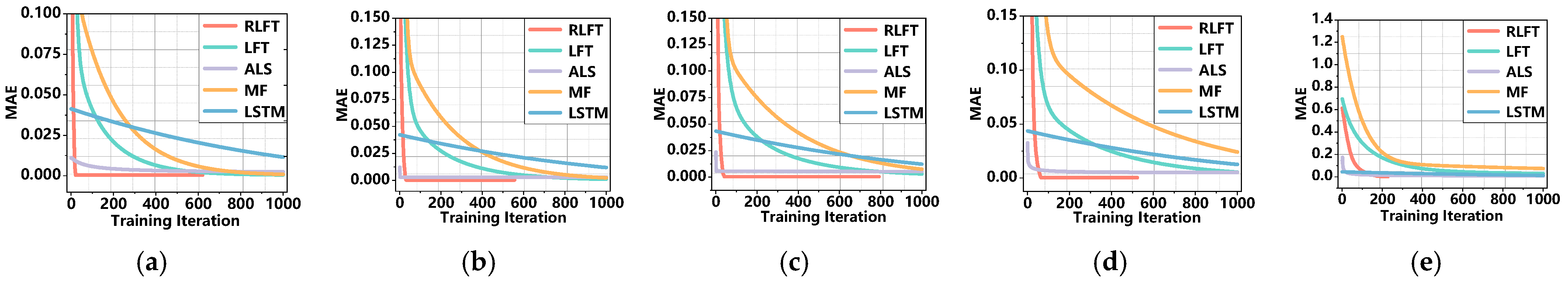
Figure 2 and Figure 3 present the training curves for all models, while Figure 4, Figure 5 and Figure 6 display the comparative results of RMSE, MAE, final iteration counts, and computational time costs across all models.

Table 5. Minimum RMSE/MAE values and convergence iteration counts for all models.

Model	Missing Rate	RMSE/Iterations	MAE/Iteration
RLFT	0.1	7.220 × 10−4/507	4.636 × 10−4/620
	0.3	7.222 × 10−4/493	4.647 × 10−4/556
	0.5	7.268 × 10−4/616	4.665 × 10−4/793
	0.7	7.276 × 10−4/473	4.675 × 10−4/523
	0.9	7.303 × 10−4/226	4.709 × 10−4/228
LFT	0.1	8.326 × 10−4/1000	5.877 × 10−4/1000
	0.3	1.594 × 10−3/1000	1.173 × 10−3/1000
	0.5	3.943 × 10−3/1000	2.974 × 10−3/1000
	0.7	7.697 × 10−3/1000	5.553 × 10−3/1000
	0.9	3.798 × 10−2/1000	2.848 × 10−2/1000
ALS	0.1	4.988 × 10−3/1000	2.535 × 10−3/1000
	0.3	6.842 × 10−3/1000	3.035 × 10−3/1000
	0.5	1.317 × 10−2/1000	5.247 × 10−3/1000
	0.7	1.811 × 10−2/1000	5.300 × 10−3/1000
	0.9	2.814 × 10−2/1000	8.218 × 10−3/1000
MF	0.1	1.191 × 10−3/1000	9.117 × 10−4/1000
	0.3	3.120 × 10−3/1000	2.441 × 10−3/1000
	0.5	9.482 × 10−3/1000	7.510 × 10−3/1000
	0.7	3.096 × 10−2/1000	2.420 × 10−2/1000
	0.9	9.382 × 10−2/1000	7.399 × 10−2/1000
LSTM	0.1	1.723 × 10−3/1000	1.160 × 10−2/1000
	0.3	1.798 × 10−3/1000	1.197 × 10−2/1000
	0.5	1.787 × 10−3/1000	1.231 × 10−2/1000
	0.7	1.912 × 10−3/1000	1.264 × 10−2/1000
	0.9	1.952 × 10−3/1000	1.286 × 10−2/1000

summarizes the RMSE and MAE performance metrics along with the corresponding final iteration numbers for each model.

Table 6. Time cost values and convergence iteration counts for all models.

Model	Missing Rate	Time Cost RMSE (ms)	Time Cost MAE (ms)
RLFT	0.1	6797	8312
	0.3	5227	5895
	0.5	4606	5930
	0.7	2906	3213
	0.9	624	630
LFT	0.1	7833	7833
	0.3	6549	6549
	0.5	4283	4283
	0.7	2600	2600
	0.9	872	872
ALS	0.1	9966	9966
	0.3	7699	7699
	0.5	5337	5337
	0.7	3301	3301
	0.9	1067	1067
MF	0.1	5206	5206
	0.3	4475	4475
	0.5	3055	3055
	0.7	1772	1772
	0.9	580	580
LSTM	0.1	2802	2051
	0.3	2389	1917
	0.5	2440	3231
	0.7	2377	2801
	0.9	2852	5199

provides detailed records of the computational time costs for all evaluated models.

Based on these results, we observe that within acceptable experimental error margins, the imputation accuracy of each model decreases as the missing rate increases. Therefore, algorithms require higher precision when handling more sparse data imputation tasks. The key findings are as follows:

• RLFT model achieves higher imputation accuracy than its baseline LFT model. As shown in Figure 4 and Table 5, RLFT attains minimum RMSE values of 7.220 × 10⁻⁴, 7.222 × 10⁻⁴, 7.268 × 10⁻⁴, 7.276 × 10⁻⁴, and 7.303 × 10⁻⁴ at missing rates of 0.1, 0.3, 0.5, 0.7, and 0.9, respectively, representing reductions of 13.29%, 54.69%, 81.57%, 90.55%, and 98.08% compared to LFT’s minimum RMSE. Similarly, RLFT’s minimum MAE values are 4.636 × 10⁻⁴, 4.647 × 10⁻⁴, 4.665 × 10⁻⁴, 4.675 × 10⁻⁴, and 4.709 × 10⁻⁴, showing improvements of 21.12%, 60.40%, 84.31%, 91.58%, and 98.35% over LFT.
• RLFT demonstrates faster convergence than the LFT at baseline. Figure 5 and Table 5 show that RLFT requires only 507, 493, 616, 473, and 226 iterations to reach minimum RMSE and 620, 556, 793, 523, and 228 iterations for minimum MAE at the respective missing rates. In contrast, LFT consistently requires a maximum of 1000 iterations to achieve both minimum RMSE and MAE across all five missing rate scenarios.
• Compared with other models,
  • RLFT achieves higher imputation accuracy than the CP decomposition-based ALS model. For RMSE, RLFT reduces values by 85.52%, 89.44%, 94.48%, 95.98%, and 97.40% at different missing rates compared to ALS. For MAE, the reductions are 81.71%, 84.69%, 91.11%, 91.18%, and 94.27%, respectively. Moreover, RLFT converges faster than ALS, which requires a maximum of 1000 iterations to reach the minimum RMSE and MAE across all missing rates. These results strongly demonstrate the superiority of latent feature decomposition over traditional CP decomposition for missing data imputation tasks;
  • RLFT shows better imputation accuracy than the MF model. The RMSE improvements are 39.38%, 76.85%, 92.34%, 97.65%, and 99.22%, while MAE shows reductions of 49.15%, 80.96%, 93.79%, 98.07%, and 99.36% at various missing rates. RLFT also converges faster than MF, which needs 1000 iterations to achieve the minimum RMSE and MAE in all cases. This conclusively proves that latent feature decomposition outperforms matrix factorization techniques, particularly in handling complex data structures;
  • RLFT exhibits superior accuracy compared to the LSTM model. It reduces RMSE by 58.11%, 59.84%, 59.33%, 61.95%, and 62.58% and MAE by 96.00%, 96.12%, 96.21%, 96.30%, and 96.34% across different missing rates. Furthermore, RLFT converges more quickly than LSTM, which requires 1000 iterations to reach optimal RMSE and MAE values. This evidence firmly establishes RLFT’s better performance in spatiotemporal feature capture compared to LSTM models.
• The RLFT model demonstrates unique advantages in computational efficiency. As shown in Figure 6 and Table 6, RLFT exhibits significantly lower time costs compared to (1) the ALS model across all missing rates; (2) the LFT model at missing rates of 0.1, 0.3, and 0.9; and (3) the LSTM model at a missing rate of 0.9. However, RLFT requires more computation time than (1) the MF model, (2) the LFT model at missing rates of 0.5 and 0.7, and (3) the LSTM model at missing rates of 0.1, 0.3, 0.5, and 0.7. Notably, RLFT converges in only 507, 493, 616, 473, and 226 iterations across different missing rates, while all other models reach the preset maximum of 1000 iterations. This demonstrates RLFT’s superior training efficiency through faster convergence. Furthermore, RLFT outperforms all comparative models in both RMSE and MAE metrics. Therefore, when comprehensively considering both convergence speed and prediction accuracy, the RLFT model demonstrates unique advantages in computational efficiency, delivering more reliable prediction results within significantly reduced timeframes. This distinctive characteristic enables substantial savings in actual training time when processing large-scale or complex datasets.

4.3. Effect of R

For the task of missing data imputation on HDI tensors, the LF dimension R affects the performance of the model based on LFT. In this section, we focus on the impact of R on the predictive accuracy of the RLFT model. Figure 7 illustrates the variation in the RLFT model as R increases from 3 to 9.

The key findings are as follows:

The predictive accuracy of the RLFT model exhibits a distinct trend as the rank R varies. As depicted in Figure 7, when the rank increases from 3 to 5, both the RMSE and MAE of the model decrease. Specifically, at rank 3, the RMSE is 7.273 × 10⁻⁴ and the MAE is 4.665 × 10⁻⁴. In contrast, at rank 5, the RMSE reduces to 7.185 × 10⁻⁴ and the MAE to 4.640 × 10⁻⁴, corresponding to predictive accuracy improvements of 1.21% and 0.54%, respectively. However, as the rank increases from 7 to 9, both RMSE and MAE exhibit an upward trend. This suggests that the model achieves optimal fitting at rank 5. Ranks that are either too high or too low may lead to suboptimal model performance. Consequently, selecting an appropriate rank value is crucial for optimizing the performance of the RLFT model in practical applications.

5. Conclusions

This paper proposes an RLFT model that incorporates the RMSprop mechanism to achieve rapid convergence and adaptive learning rate adjustment during training. By using structural state data from scaled bridge models as test cases, the experimental results demonstrate that the RLFT model comprehensively outperforms the comparison models (LFT, ALS, MF, and LSTM) in both imputation accuracy and convergence speed, proving its superiority in handling complex data structures and capturing spatiotemporal features.

However, several aspects of our work require further improvement:

• Computational efficiency optimization: Although the RLFT model shows certain advantages in time consumption, there remains room for enhancement.
• Manual hyperparameter adjustment: The model currently requires manual tuning for different missing rates or datasets, indicating the need for more efficient parameter optimization methods.

To address these limitations, future work will focus on further model optimization to achieve more efficient training and more accurate predictions. Notably, the imputation of continuously missing data presents another valuable research direction worthy of investigation.

In future work, we will delve into the effectiveness of RLFT in handling consecutively missing data. Though RLFT works well for random missing data, data loss in SHM is not always random. So, we need to test how RLFT performs in such cases. We will create experiments to mimic non-random missing data scenarios. This will let us evaluate RLFT’s data imputation accuracy and convergence speed in these situations and see how it affects the final monitoring results. Meanwhile, we plan to incorporate bias terms into the RLFT model to address measurement errors and uncertainties, thereby enhancing its robustness.

In addition, we will evaluate the applicability of RLFT in online or real-time SHM applications. As SHM systems typically require real-time structural health monitoring, the real-time performance of the method is crucial. We will explore how RLFT performs in real-time data processing, including its adaptability to data streams, processing speed, and stability and accuracy in real-time monitoring environments.

We plan to conduct integrated tests with existing online monitoring systems to verify the practicality and efficiency of RLFT. This will involve making necessary algorithmic adjustments to ensure that RLFT can operate efficiently in resource-constrained real-time systems and provide timely monitoring feedback. Through this work, we hope to further promote the application of RLFT in the field of SHM and offer more guidance and references for future research and practice.