S-EPSO: A Socio-Emotional Particle Swarm Optimization Algorithm for Multimodal Search in Low-Dimensional Engineering Applications

Abstract

This paper examines strategies aimed at improving search procedures in multimodal, low-dimensional domains. Here, low-dimensional domains refers to a maximum of five dimensions. The present analysis assembles strategies to form an algorithm named S-EPSO, which, at its core, locates and maintains multiple optima without relying on external niching parameters, instead adapting this functionality internally. The first proposed strategy assigns socio-emotional personalities to the particles forming the swarm. The analysis also introduces a technique to help them visit secluded zones. It allocates the particles of the initial distribution to subdomains based on biased decisions. The biases reflect the subdomain’s potential to contain optima. This potential is established from a balanced combination of the jaggedness and the mean-average interval descriptors developed in the study. The study compares the performance of S-EPSO to that of state-of-the-art algorithms over seventeen functions of the CEC benchmark, and S-EPSO is revealed to be highly competitive. It outperformed the reference algorithms 14 times, whereas the best of the latter outperformed the other two 10 times out of 30 relevant evaluations. S-EPSO performed best with the most challenging 5D functions of the benchmark. These results clearly illustrate the potential of S-EPSO when it comes to dealing with practical engineering optimization problems limited to five dimensions.

1. Introduction

Solutions to practical engineering problems often lie in multimodal and multi-optima landscapes [1]. Although identifying an efficient answer to a practical problem generally only requires a single good solution, having access to several sets of potential configurations allows designers to make completely enlightened selections among solution groups possibly offering nonessential but beneficial characteristics.

Moreover, numerous contexts, such as those defined by mechanical design problems, entail intricate interactions among variables [2], resulting in complex optimization tasks. Consequently, the ensuing calculation burdens and associated simulation times still impose limitations on the number of optimization variables. The following publications present investigations on the optimization of mechanical systems [3,4,5,6,7,8,9,10]. They indeed provide a good depiction of the context. For instance, Refs [3,4] evaluate the performance of various metaheuristic algorithms covering typical mechanical problems. The systems they examine involve between two and eleven design variables. The research in [5,6,7,8,9] also considers a variety of typical mechanical systems and problems. These include the design of gearboxes [5,6], springs, and welded joints [7], among others, and aim to optimize grinding operations to minimize production costs and maximize surface quality [7]. More specifically, Ref. [7] proposes an algorithm targeting the optimization of real-life applications. These recent papers also set out to identify optimal parameter settings in laser cutting operations [8] and to define optimal gear-shifting strategies minimizing fuel consumption in internal combustion engine vehicles [9]. Most importantly, regardless of their complexity, all these optimization studies involve not more than five variables.

The number of variables has an even greater impact in optimization jobs involving contact simulations, such as the optimization of gear tooth profiles or bearing roller profiles, since they can quickly become very computation-intensive [10]. Optimization problems involving such mechanical elements are often limited to fewer than five variables.

Since the current literature indicates that they define a significant proportion of the everyday optimization jobs in engineering, and because improving the dedicated optimization methods remains an open research challenge, this article focuses on configurations of this type, which may be designated as multimodal problems of relatively low dimensionality. The work develops and analyses some strategies designed to improve the performance of search procedures over multimodal landscapes comprising multiple optima. While all the strategies considered can be individually adapted and integrated within any existing algorithm, the exercise of assembling them results in an optimization algorithm that is highly competitive.

1.1. Research Question

A recognized approach to help search procedures form stable subpopulations around potential multimodal domain zones integrates niching ability into standard search algorithms [1]. For instance, when applied to the particle swarm optimization algorithm (PSO), this strategy leads to efficient adaptations [1]. However, most often, it results in methods requiring predetermined information on the landscape structure to define their niching control parameters [1]. Their ultimate efficiency thus depends on the quality of pre-existing descriptions.

In other words, the search performance of many algorithms is subject to specific constraints which control individual freedom, namely, a niche radius or a guided interaction with closest neighbours.

On the other hand, the question may be asked as to whether a similar efficiency could be obtained without restricting the freedom of the agents. Rather than imposing restrictions, could giving particles unique abilities or personalities and allowing them to perform specialized search operations be a more fruitful approach? The terms individual and agent refer to a candidate solution. In PSO, particles are considered intelligent individuals. This paper adopts the term particle to refer to any type of agent, regardless of the metaheuristic being considered.

The Grey Wolf algorithm [11] is a good example of a model involving specialized particle types. The strategy underlying this algorithm divides the particle groups, each one respecting a ruled behaviour. Similar strategies have been integrated into various models, with the Whale optimization algorithm published in [12] by the same authors being a good example. The most interesting feature brought in by these models is allowing a distinct and complementary contribution by the particle groups.

Nevertheless, the fact is that the distinct role of the particle does not emanate naturally from its personality in a free context, but rather, is imposed via specific tasks. Hence, the task definition is somewhat more related to the nature of the search space, which is a unique optimum landscape in [11,12]. Therefore, it may be assumed that changing the configuration to a multiple optima domain would require a significant restructuring of the task sets. Conversely, one may imagine that integrating specific characteristics into the personality of the particles themselves would allow them to develop specialized search responses or behaviours that are self-adaptable to landscape changes.

1.2. Research Contribution and Paper Organization

To explore this avenue and eliminate the need for predefined niching parameters to locate and maintain multiple optima, the present paper develops the following strategies:

• The first endows the particles with socio-emotional personalities. Based on an analogy pertaining to socio-emotional relations prevailing during the mammal reproduction period, the proposed approach introduces three particle types with specific personalities. Among these, some male particles are intrepid and explore the landscapes, while others are more prudent and preserve the found optima. The interactions between the socio-emotional particles give the swarm a natural ability to locate and maintain multiple optima and completely eliminate the need for predefined niching parameters.
• The second strategy introduces a technique to help the particles visit secluded zones. This technique apportions the particles of the initial distribution to subdomains based on biased decisions. The biases reflect the subdomain’s potential to contain optima. The procedure establishes this potential from a balanced combination of the jaggedness and the mean-average interval descriptors put forward in the study.
• In addition, to control the number of particles required to populate the subdomains, the proposed investigation reduces the domain dimensionality based on a sensitivity index.
• To boost the performance of the particles, the investigation also examines an economical strategy exploiting the information provided by contours formed by surrounding particles.

After the literature survey presented in Section 2, the following sections detail the four strategies mentioned above (Section 3, Section 4 and Section 5). Section 3 begins with the pseudocode of the complete optimizer to show how combining these approaches leads to the proposed algorithm. This algorithm is designated as the Socio-Emotional Particle Swarm Optimizer or S-EPSO. Finally, Section 6 compares the performance of S-EPSO to those of two state-of-the-art algorithms over seventeen multimodal functions with multiple optima. Section 6 also demonstrates the S-EPSO’s ability to deal with real-world constrained optimization problems.

2. Related Work Survey

The problem of searching for optimal solutions over multimodal landscapes is certainly not new, and the literature on the topic is rich. Published more than a decade ago, Ref. [1] offers a detailed description of an already great literature on the subject. Since that review continues to be valid, the present paper does not therefore repeat the discussion.

In Ref. [1], Li integrated a ring neighbourhood topology into PSO and demonstrated that restricting the particle interactions to some close neighbours leads to stable niche formation without any prior knowledge of the searched space. In particular, the control of the particle interactions eliminates the need for a pre-established niche radius. This result represents a clear and strong advantage. Essentially, the algorithm developed in [1] responded to the following:

(1)

Require no specification of niching parameters;

(2)

Must be able to locate and maintain multiple optima;

(3)

Must be able to locate multiple global and local optima;

(4)

Have low computational complexity.

The validation of the algorithm performance in [1] includes fourteen test functions. The validation procedure compares the proposed algorithms to high-performing niching PSO variants. The comparison is mainly based on a success rate measure (SR) defined as shown in Equation (1).

$$SR=numberofrunsfindingalloptima/numberofruns$$

(1)

Globally, the reported SR values are very high for the easiest functions. On the other hand, while SR remains over 90% for the ring topology algorithms, it drops significantly with the 3D case for the 2D Shubert function. When considering the Vincent function, practically all algorithms included in the analysis performed poorly, even in the 2D case.

Almost simultaneously, Epitropakis et al. [13] presented an alternative approach developed for the Differential Evolution (DE) algorithm and the mutation schemes DE/rand/1 and DE/rand/2 [14,15,16]. The authors proposed the two new mutation operators, DE/nrand/1 and DE/nrand/2, designed to improve the ability of the DE algorithm to converge toward and maintain multiple optima, over multimodal landscapes. Essentially, the proposed mutation variants incorporate the nearest neighbour influence into the mutation operators to force the particles to explore their neighbourhood. As in the case of the ring topology with PSO, the incorporation of neighbour-mutation operators to DE eliminates the need for predefined niching parameters. The authors of [13] used eight 2D multimodal functions to validate the resulting algorithms. The validation procedure comprised two measures: SR and the peak ratio (PR), defined as written by Equation (2):

$$PR=numberofpeaksfound/actualnumberofpeaks$$

(2)

The validation shows that the two new versions of the DE algorithms (DE/nrand/1-2/bin) compare rather well with the five other algorithms included in the process. Nevertheless, the results show that all the tested approaches demonstrate significant difficulties with the Shubert and Vincent functions. However, the new algorithm DE/nrand/2 provides good performance with the Shubert function. On the other hand, none of the algorithms performs well with the Vincent function.

Later, Ref. [17] introduced a 20-function benchmark to evaluate and compare niching methods. The benchmark included simple 1D and 2D functions, the Shubert and Vincent (2D and 3D) functions, and more complex composition functions (2D up to 20D). In addition to SR and PR, the authors suggested the convergence speed as a performance measure. The convergence speed corresponds to the Average number of Function Evaluations (AFE) required to identify all global optima at a selected accuracy level $ϵ$. Equation (3) formulates the measure:

$$AFE={\sum }_i^{NR}{FE}_i/NR$$

(3)

where FE_i is the number of Function Evaluations required by a run i, and NR denotes the number of runs. Ref. [17] also presented the performance of two baseline models: the DE/nrand/1 and the Crowding DE/rand/1 algorithms developed in [13,18], respectively. Moreover, instead of prescribing any population size, the authors preferred a Maximum number of Function Evaluations (MFE).

As in the previous studies [1,13], the obtained results show good performances of the algorithms with the simple functions, and less successful predictions with the Shubert and Vincent functions, even with the 2D versions. When considering the 2D versions of the composition functions, DE/nrand/1 slightly improves its prediction quality, whereas Crowding DE/rand/1demonstrated a significant effectiveness decrease.

More recently, Wang et al. [19] published a performant version of the niching DE algorithm. The procedure essentially incorporates three techniques within the base algorithm: 1- An automatic niching method that eliminates the need for pre-decided cluster characteristics and that helps detect multiple optima. A dimensional reduction procedure also helps this niching method deal with high-dimensional domains; 2- A contour prediction strategy exploiting the available information to improve the convergence rate; and 3- A local search designed to enhance the result accuracy. The authors apply the final procedure to the twenty functions of the Ref. [17] benchmark, and compare its performance with those of state-of-the-art algorithms, including the winner of the CEC 2015 competition published in [20]. This last model depends on several interconnected particle swarms simultaneously optimizing local subdomains [20]. The results presented in these two references demonstrate performance that is largely improving the results described above for the Shubert and Vincent functions. Indeed, the performance of the algorithms remains very good overall, up to the 5D version of the most challenging composition functions of the benchmark.

The following sections show how the combination of the proposed strategies meets the requirements provided in the list of specifications above extracted from [1].

3. Particle with Socio-Emotional Behavior and Model Basis

An efficient search procedure must preserve an appropriate balance between exploration and exploitation over the complete process evolution [21,22]. In multimodal optimization, the situation is even more intricate; at the search beginning, the procedure must simultaneously provide a sufficient level of exploration to avoid premature convergence and preserve the identified promising zones. Later in the progression, the model must explore all optima neighbourhoods and ultimately gather the particles in multiple clusters at the different positions of the global optima. The specific behaviour required for a successful operation may be ascribed to different particle personalities interconnected via a particular sociological attraction between them.

3.1. Pseudocode of the S-EPSO Algorithm

The present section corresponds to point 1 of the introduction. To enhance the descriptions, it begins with Figure 1, which describes the pseudocode of the S-EPSO algorithm. In order to facilitate the duplication of the model or parts of it, the pseudocode is voluntarily extensive. The presentation divides the algorithm into two parts. Part A groups the Initiation steps, while Part B describes the Computation steps. Numbers also mark the beginning positions of operation groups.

As already indicated, the proposed model draws an analogy to the socio-emotional dynamic prevailing during mammalian reproduction. The system presented is a strong simplification of real socio-emotional interactions. It assumes a society comprising one female personality type searching for the best male partners, and two male personality types searching for female partners. Each male type also has a specific charisma score. The sage male type searches for the best females in his close neighbourhood, while the adventurous male type prefers to search for the best female far from his neighbourhood.

Adventurous males tend to have shorter lifespans, while sage males generally live longer. However, more resilient adventurous males may transition into sage roles, whereas frail sage males may die prematurely. Additionally, adventurous males often exhibit greater charisma, making them more attractive to females compared to sage males.

In addition, the particle community evolves over landscapes where each other’s view may be affected by environmental factors, such as the fog in the Firefly algorithm introduced by Yang in [23] for unimodal domains.

From a more technical perspective, the quality of a female or a male refers to their response to the objective function. Thus, a strong adventurous male is in a good position in the domain, whereas a frail sage male is located at a position in the domain where the function value is less competitive than the values found by the other males.

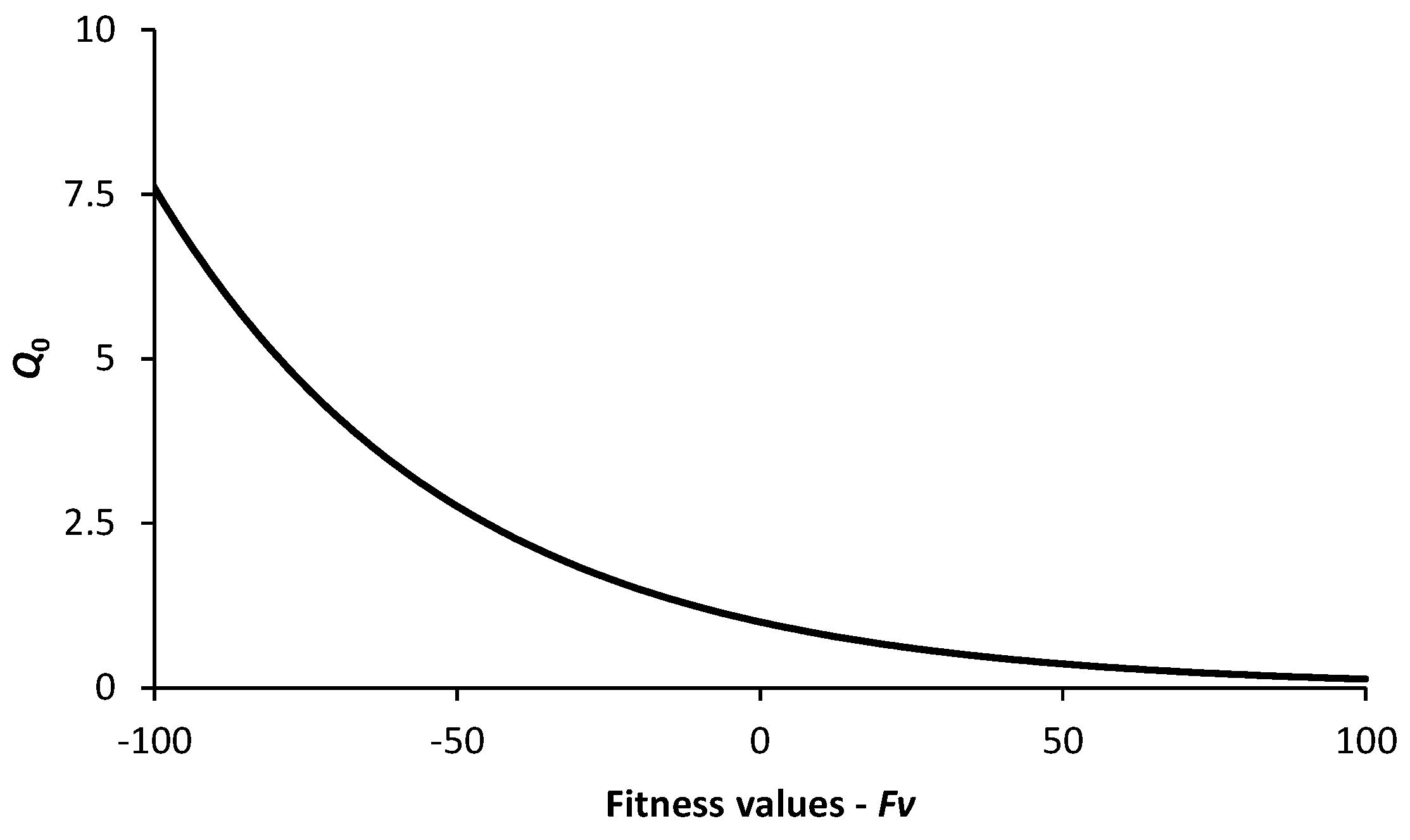
3.2. Algorithm Basis and Socio-Emotional Particle Personalities

The particle types provide three levels of exploitation/exploration: the less mobile sage males provide more exploitation; the adventurous males offer high levels of exploration and are responsible for detecting multiple optima.; the females provide an intermediate level of exploitation/exploration, and are responsible for transferring the good spots located by the adventurous males to the sage males.

The haziness (designated below as ${\gamma }^{*}$) introduced into the process promotes the exploitation of the domains and forces both the females and sage males to better probe their neighbourhoods. In clear, the interactions between the females and sage males in a hazy environment introduce a natural formation of niches in the vicinity of optima. The particles’ attractiveness ($\beta$ defined by Equation (7)) controls these interactions. The swarm is endowed with an ability to locate and maintain multiple optima without any predefined niching parameters. On the other hand, the landscape haze does not affect the adventurous male vision. Besides, their shorter life allows for reducing the exploration level approaching the end of the search evolution.

Although the preceding description appears to veer significantly from that of existing models, it remains close to the PSO-local-best versions formulated to generate multiple niches around optima [1].

Indeed, the core of the proposed algorithm corresponds to the PSO-local-best formulation. Equations (4) and (5) describe this PSO version. At each iteration t + 1, the model tries to move a particle i closer to an optimum of the D dimensional domain. The progression of the particle depends on a memory term specified by the best position p_best i it has visited thus far, and the location l_best (t) of the best particle of its neighbourhood identified during iteration t. The influence of these contributors is adjusted by random factors. The model formulation also integrates the inertia of the particles. Equation (4) translates this depiction and expresses the velocity v_id(t+1) at iteration t + 1 of particle i along each dimension d of the D domain. Parameter W represents the constant inertia weight of the previous advance of the particle (0 ≤ W ≤ 1), c₁ and c₂ are acceleration constants (≈2), and ${\epsilon }_{1\left(t\right)}$ and ${\epsilon }_{2\left(t\right)}$ are random numbers between 0 and 1. Equation (5) establishes the new position x_id(t+1) of particle i along dimension d:

$$v_{id(t+1)}=W{v}_{id\left(t\right)}+{c_1\epsilon }_{1\left(t\right)}\left(l_{bestid}-x_{id\left(t\right)}\right)+{c_2\epsilon }_{2\left(t\right)}\left(p_{bestid}-x_{id\left(t\right)}\right)$$

(4)

$$x_{id(t+1)}=x_{id\left(t\right)}+v_{id(t+1)}$$

(5)

The first and last terms of the right-hand side of Equation (4) represent the particle record, while the middle term introduces the particle’s social interactions with the swarm. This middle point is therefore the position where the particle’s socio-emotional personality should be defined. It should also introduce the particle’s ability to navigate and locate other particles in a hazy space.

In the Firefly algorithm published in [23], Yang related the attractiveness β of a particle or a firefly j to the intensity of its light emission I detected at a distance r_ij by a second firefly i, where r_ij is the Euclidian distance between firefly i and firefly j $r_{ij}=\sqrt{{\displaystyle \sum _{d=1}^D{\left(x_{jd}-x_{id}\right)}^2}}$. The light intensity at the source I₀ of firefly j reflects its response to the objective function O(x_j). Thus, in a foggy landscape defined by a light absorption coefficient γ, $I(r)=I_0{e}^{-\gamma r^2}$ gives I at a distance r from the source particle. Hence, when rewritten in terms of attractiveness, this expression becomes $\beta (r)={\beta }_0{e}^{-\gamma r^2}$, where β₀ is the particle’s attractiveness at the source. Low values of γ describe clear skies with the firefly being highly visible, while high γ values lead to a reduction of the visibility or attractiveness of the firefly. Finally, Firefly establishes the position change of particle i attracted by a brighter particle j, as indicated by Equation (6). In this equation, Rf denotes a random contribution driving the domain exploration:

$${(x_{id})}^{\prime }=x_{id\hspace{0.17em}(t)}+\beta (r)\left(x_{jd\hspace{0.17em}(t)}-x_{id\hspace{0.17em}(t)}\right)+Rf$$

(6)

Although the original Firefly version was designed to operate on unimodal landscapes and to locate a single global optimum, the attractiveness definition proposed in [23] provides the algorithm with a natural clustering tendency. Thus, the strategy proposed in the present study adopts a similar approach to define the particles’ socio-emotional personalities and to replace the social term in Equation (4).

Equation (7a) formulates the attractiveness of a male to a female particle (β_fm), while Equation (7b) gives the attractiveness of a female for a sage male (β_smf). Finally, Equation (7c) formulates the attractiveness of a female to an adventurous male particle (β_amf):

$${\beta }_{fm}(r)=\exp \left(-\left({\displaystyle \frac{\gamma *}{Ch}}\right){\left({\displaystyle \frac{r}{L_e}}\right)}^2\right)$$

(7a)

$${\beta }_{smf}(r)=\exp \left(-\gamma *{\left({\displaystyle \frac{r}{L_e}}\right)}^2\right)$$

(7b)

$${\beta }_{amf}(r)=\left(1-a\right){\sin }^m\left({\displaystyle \frac{\pi r}{2L_e}}\right)+a$$

(7c)

In Equation (7), r is the Euclidian distance and ${\gamma }^{*}$ is the medium haziness coefficient equivalent to the light absorption coefficient in Firefly. Moreover, as indicated in [10], since ${\gamma }^{*}$ is a dimensionless variable, to respect the principle of dimensional homogeneity, r, which is the particle separation distance should also adopt a dimensionless form. This variable must be adapted to the probed landscape. The diagonal of the D-dimensional domain (L_e) is probably the best variable to use to define the dimensionless distance (Figure 1, Part A). Parameter Ch in Equation (7a) denotes the charisma of a male type. A value greater than one augments the visibility of a particle in hazy environments. Equation (7c) shows that the visibility of the female particles to the adventurous male type is not affected by the landscape haze. Equation (7c) produces values $\in \left\{\left(1-a\right)\mathrm{t}\mathrm{o}1\right\}$ which increase with the dimensionless distance ${\displaystyle \frac{r}{L_e}}$. Factors a and m are two constant parameters. Parameter $a\in \left\{0\mathrm{t}\mathrm{o}1\right\}$ introduces an offset of the function. For example, $a=0$ results in 0 attractiveness for close female particles ($r\cong 0$), whereas $a=1$ generates an attractiveness of 1 for all female particles regardless of r. On the other hand, m controls the curvature of the attractiveness function. It may be set at any amplitude $\in \left\{0\mathrm{t}\mathrm{o}\infty \right\}$. The recommended range, however, is $\left\{0\mathrm{t}\mathrm{o}5\right\}$. Figure 2 illustrates the dimensionless attractiveness established with Equation (7); Figure 2a shows the attractiveness of males with a charism Ch = 2 calculated for females by Equation (7a), as well as the female attractiveness calculated for sage males with Equation (7b), while Figure 2b presents the female attractiveness given by Equation (7c) for adventurous males. The dimensionless distance ${\displaystyle \frac{r}{L_e}}$ ranges from 0 to 1. For Equations (7a) and (7b), ${\gamma }^{*}$ is set at three values, namely, 0.5, 50, 1000 and 10,000, while for Equation (7c), a is set at 0 and 0.2, and m at 0.5, 1.5 and 5.

Figure 2a shows the impact of ${\gamma }^{*}$ as well as the accrued visibility of males with a charisma greater than one. For the highest ${\gamma }^{*}$ included in the graph, the male charisma has no practical effect, and the females and sage males demonstrate similar attractiveness levels. Finally, Figure 2b clearly shows the low attractiveness of females close to an adventurous males as well as the role of a that sets the minimum attractiveness level.

Equation (8) writes the formulation proposed to replace Equation (4) in the proposed algorithm. In this formulation, the variables defined previously remain unchanged, whereas ${\beta }_{ij}$ is calculated from Equation (7) for each particle type. When introduced in Equations (5) and (8) establishes the particles’ evolution:

$$v_{id(t+1)}=W{v}_{id\left(t\right)}+{\epsilon }_{1\left(t\right)}{\beta }_{ij}\left(r_{ij}\right)\left(x_{jd\left(t\right)}-x_{id\left(t\right)}\right)+{c_2\epsilon }_{2\left(t\right)}\left(p_{bestid}-x_{id\left(t\right)}\right)$$

(8)

Equation (8) (Figure 1, Part B-10) maintains the influence of the memory and the inertia of particle i in the calculation of its progression, while the attraction of a single particle j defines the social term. Particle j represents the most alluring particle detected by i at a distance r_ij (Figure 1, Part B-6 and 9). The appealing quality of j for i corresponds to the combination $Q_0{\beta }_{ij}$, where Q₀ represents the quality of a particle and is similar to I₀ in Firefly. It thus results from the particle’s response to the objective function. Therefore, among all particles j satisfying the condition (Q_0j > Q_0i), the most alluring one for particle i is the one maximizing $Q_0{\beta }_{ij}$.

$$Q_0(Fv)={k_0}^{\left({\displaystyle \frac{-Fv}{k_1}}\right)}$$

(9)

This approach also helps avoid potentially fruitless function evaluations. Indeed, any male particle i unable to detect a female partner j offering a quality Q_0j > Q_0I stays still. Conversely, to maintain a minimal evolution of the swarm, females in the same situation simply move as a result of their impetus introduced in Equation (8) by the memory and the inertia terms.

In a maximization problem, I₀ may be set equal to the fitness value (Fv) [23]. However, the present study considers minimization problems. For fitness values $Fv\ge 0$, the light intensity may be calculated as $I_0={\displaystyle \raisebox{1ex}{$1$}\!\left/ \!\raisebox{-1ex}{$1+Fv$}\right.}$ [10]. This formulation is nonetheless not valid for $Fv<0$. Hence, the literature offers few alternatives. For example, [24] suggests that when $Fv<0$, $I_0=1+\left|Fv\right|$.

To avoid introducing any abrupt modifications during the conversion of the fitness value into attractiveness, and thus to the resulting impact on the particle interactions, it may be suggested that an appropriate formulation should describe a low-order function, ensuring, a least, a continuous second derivative. The combination of the above two formulas for $I_0$ as proposed in [24] does not respect this condition. Thus, the present study instead suggests determining Q₀ using Equation (9), where k₀ and k₁ are two constants, respectively set at 1.5 and 20.

Figure 3 draws Equation (9) over a [−100 to 100] range of Fv. This plot shows that while the conversion induces a beneficial promotion of the low fitness values, it does not produce any strong slope changes.

3.3. Life Expectancy of the Particles

Besides their respective personalities, the two male types also have different lifespans. The adventurous males are responsible for the domain exploration; therefore, their contribution should decrease toward the end of the search process. The common approach is to reduce the exploration level by controlling the search process itself. However, in the proposed model, this control is induced by removing short-lived particles, mainly the adventurous males.

Nevertheless, it is crucial that the reduction in the number of males does not lead to a decline in the overall quality of knowledge. Therefore, the elimination process begins with those offering the lowest quality. However, adventurous males may become sages if they find a particle of lower quality to replace. In this way, they can preserve their positions, while the weakest potential solutions simply vanish.

After establishing the proportion of the total particle number (N) belonging to the female (ζ) and male (1 − ζ) groups, as well as the proportion of the adventurous (κ) and sage (1 − κ) males forming the second particle group, the process sets the life expectancy control.

This initial proposal first sets the minimum life expectancy of the short-lived males at a fraction ($\chi$) of the total pre-established maximum number of iterations (MaxNI). After $\chi MaxNI$ iterations, a group of $\kappa \left(1-\zeta \right)N$ short-lived males start dying (Figure 1, Part B-1). This period extends over half of the remaining iterations, or ${\displaystyle \frac{1}{2}}\left(1-\chi \right)MaxNI$ iterations. The males vanish at a constant rate $Vr={\displaystyle \frac{2\kappa \left(1-\zeta \right)N}{\left(1-\chi \right)MaxNI}}$. Thereafter, the remaining ${\displaystyle \frac{1}{2}}\left(1-\chi \right)MaxNI$ iterations involve $\zeta N$ females and $\left(1-\kappa \right)\left(1-\zeta \right)N$ sage males exploiting the identified most promising zones and gathering in clusters around the optima. During this last period, the exploration capacity of the females decreases, and their exploitation ability increases to reach those of the sage males. The adventurous male disappearance eliminates both the high and intermediate exploration levels.

3.4. Boundary Crossing

Along with the particle interactions, the method adopted to handle boundary crossings occurring during the progression of the particles can strongly affect the search performance of an algorithm. The literature offers numerous procedures to deal with this aspect, with the random, the reflecting and the absorbing methods being some of the most popular approaches [25]. These strategies present some drawbacks, as discussed in [25]. In addition, in algorithms such as PSO, a boundary-crossing correction affects both the particle position (Equation (5)) and its velocity (Equation (4)). Therefore, to prevent cascading adjustments, the authors of [25] suggested that only correcting the particle position and omitting velocity adjustments should be sufficient. Although the proposed algorithm involves a structure equivalent to that of PSO, the approach adopted in the present context controls the velocity and also adjusts the position of the particles crossing a domain boundary.

First, the proposed scheme limits the velocity amplitude, as indicated in Equation (10) (Figure 1, Part B-10). In Equation (10) L_d denotes the domain length along dimension d. More importantly, however, to grant the model the ability to concurrently detect multiple optima located close to and exactly on the boundary, as well as distributed across the search space, efficiently, the adopted correction relocates the particles reaching outside a dimension d of the search domain at a random position between their starting position and the boundary. Figure 4 illustrates this description, while Equation (11) formulates it, where ${\epsilon }_{3\left(t\right)}$ is a random number between 0 and 1 and l_d is the coordinate of the boundary along the d-axis:

$$v_{id(t+1)}=\left\{\begin{array}{c}{L}_{d}if{v}_{id(t+1)}>L_d\\ {-L}_{d}if{v}_{id(t+1)}<{-L}_d\end{array}\right.$$

(10)

$$x_{id(t+1)}=x_{id\left(t\right)}+{\epsilon }_{3\left(t\right)}\left(l_d-x_{id\left(t\right)}\right)$$

(11)

3.5. Additional Information

The algorithm described above is first designed to operate over multimodal landscapes having multiple optima. Larger ${\gamma }^{*}$ values such as 1000 or 10,000 (Figure 2a) restrain the sage males’ mobility and force a clustering response. However, the same algorithm should also perform very well over single optimum domains. Indeed, low values of ${\gamma }^{*}$ such as 0.5 practically eliminate the mobility restrictions imposed on the sage males (Figure 2a), and consequently, on the females. They move freely and are thus able to gather around a single position. On the other hand, the adventurous males still maintain high exploration levels. Obviously, ${\gamma }^{*}$ renders the algorithm completely versatile.

As already indicated, multimodal landscapes often contain optima in zones close to their boundaries. Hence, regardless of the adventurous males’ agility, the restriction imposed on the sage males by higher ${\gamma }^{*}$ may prevent them from accessing particular zones of a search domain. The following sections present a complementary strategy designed to improve the model probing efficiency.

4. A Strategy Based on a Segmentation of the Search Domain’s

When the swarm contains particles with constrained mobility, the role played by the initial particle becomes more important. Indeed, it may become difficult to attract sage males to secluded zones briefly visited by peripatetic males, since the attraction must first transit via female particles. Thus, to ensure a minimal coverage of the domain, a uniform initial distribution appears to be the foremost option. However, depending on the particular number composing the swarm, this approach may result in particle positions still too far from the domain limits. Nevertheless, the uniform initial distribution approach may be improved by a segmentation of the search space.

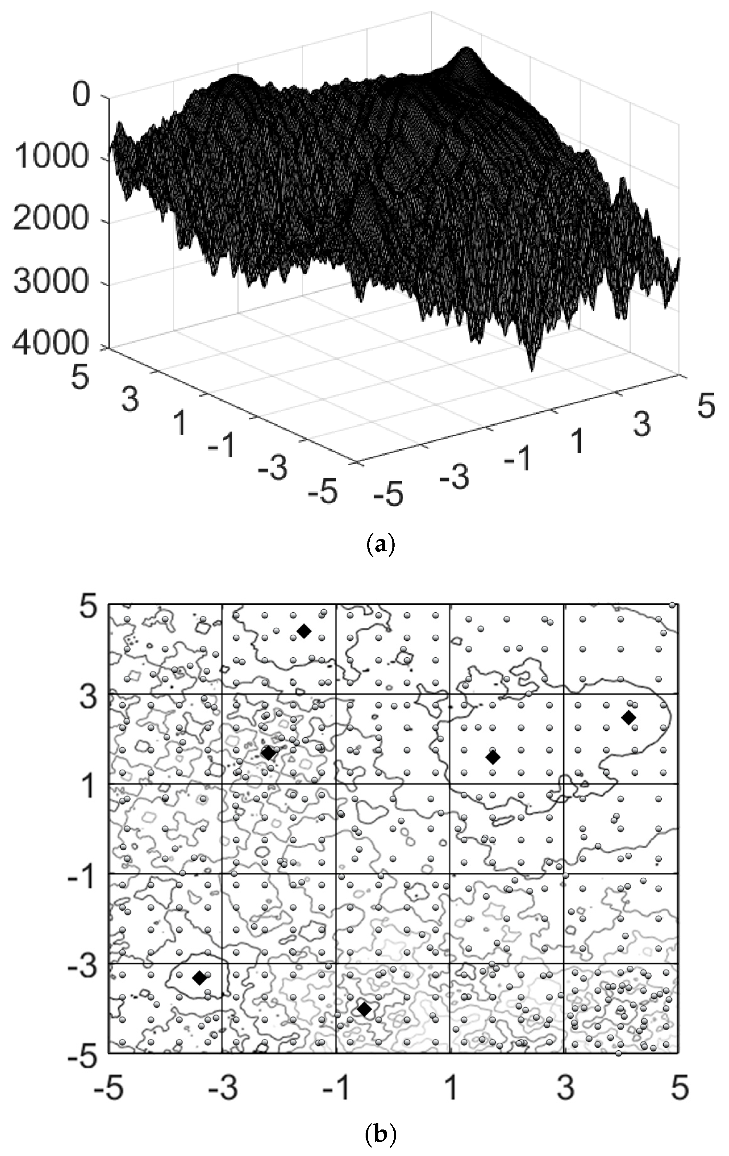
4.1. Problem Description

The present section refers to point 2 of the introduction. It describes the procedure introduced in Part B-2 in Figure 1. Figure 5 presents the corresponding pseudocode. The illustration again divides the algorithm into two parts. Part C corresponds to the dimensionality reduction steps, while Part D describes the Distribution tasks. Numbers also mark the beginning positions of the operation groups.

It is worth mentioning here that Part D-4 decides the particle type based on the generation order: the females compose the first segment of the distribution, the sage males, the second, and the intrepid males, the last. Since the segment order in the distribution does not change during the iterations, it tags the particles with their precise types.

The proposed technique divides the domain into S regular segments along each D dimension. The procedure first uniformly apportions the particles to the resulting S^D subdomains. Then, it uniformly distributes them over each subdivision (Part A in Figure 1). Depending on the number of particles and the domain dimensions, the distribution process may produce some remaining individuals. Thus, at the end of the process, these remainders are individually assigned to random positions of the landscape.

While this uniform distribution operation may significantly help the scan evolution, it remains insufficient to guarantee an always fully successful search. Rather, it serves as the first step in the preparation of the initial distribution of the individuals over the landscape. Moreover, in practice, any augmentation of the probed domain dimensionality will strongly affect this strategy. The authors of Ref. [19] faced a similar situation with the automatic niching ability of their algorithm.

To solve the problem, the authors of [19] first reduced the domain dimensionality via a Principal Component Analysis (PCA). Since the domain segmentation introduced herein and defined by the S^D subdomains would rapidly require unmanageable numbers of particles, the second step (Part C in Figure 5) aims to reduce the problem dimensionality. It should reduce the number of dimensions considered during the segmentation from D to D*. Therefore, instead of S^D, the operation will involve S^D* subdomains. Based on the Ref. [19] suggestion, the maximal value for D* here is three. Thus, if $D\le 3$, then $D^{*}=D,$ otherwise $D^{*}=3$.

The third step (Part D in Figure 5) aims at apportioning the particles to the S^D* subdomains more efficiently, or, more specifically, apportioning the particles based on biased decisions established during pre-evaluations of the potential of the subdomains. The first uniform particle distributions made over each subdomain allow pre-probing of their worth. The evaluation of the potential of a zone is ultimately similar to the optimization process itself. Given its role, the pre-probing step must thus offer a rough but reliable description at the lowest possible computation cost.

When observing landscapes such as the 2D Vincent function (36 minima) illustrated in Figure 6a, it appears that the potential of a zone to contain multiple optima can be depicted and evaluated by its jaggedness. On the other hand, when looking at the 2D Himmelblau function (4 minima) presented in Figure 6b, it seems clear that in the context of minimization, the jaggedness aspect has no bearing and cannot serve in a pre-probing strategy. In fact, a comparison of the function local or subdomain means to the overall average would be preferable to pre-identifying the zones closer to the four minima. On the contrary, the means of the subdivisions would provide no valid insights into the nature of the Vincent function, since it essentially combines sine functions.

From a general perspective, because various landscapes can present different combinations of these two descriptions (jaggedness and subdivision mean), we may imagine that a proper association of the jaggedness and subdivision means evaluations should be sufficient for an efficient and low-cost pre-probing of various landscapes and should thus provide serviceable pre-mappings of the domains’ potential. The ultimate goal is then to associate these measures in a balanced description to form the weight factors required to generate initial particle distributions properly reflecting the subdomain potential. For clarity, the next three subsections first detail this pre-mapping strategy and end with the dimensionality reduction aspect.

4.2. Evaluation of Landscapes Jaggedness

The Jaggedness (J) considered here also refers to the frequency spectrum representing the landscape. While a precise representation of the frequency spectrum of a D-dimensional domain is not easy, a 2D landscape provides a simple illustration of the concept, which then becomes equivalent to surface roughness. Hence, high energy levels at higher frequencies should reflect a higher jaggedness of surfaces. However, while a Fast Fourier Transform (FFT) would normally provide the required information, in the present context involving D-dimensional domains, obtaining a low computation cost evaluation remains challenging.

The proposed strategy is close to the quantitative method put forward in 1970 by Hjorth for EEG activity evaluation [26]. The Hjorth method aimed at predicting properties of time signals in the frequency domain from time-based measures of physical parameters. The author proposed three parameters: Activity, Complexity and Mobility. These parameters are also described as normalized slope descriptors [27]. The first reflects the squared standard deviation of the signal amplitude. It thus evaluates the mean power. Complexity provides an evaluation of the signal bandwidth. Finally, Mobility is designed to provide an estimate of the mean frequency of the signal [27]. Mobility thus offers information closely related to the needs of the present study.

If a time signal T(t) is known by n sample values ${\tau }_u$, Activity (A) is expressed as $A^2={\displaystyle \frac{1}{n}}{\sum }_{u=1}^n{\tau }_u^2$, and when defining ${\delta }_u={\tau }_{u+1}-{\tau }_u$, Mobility (M) is expressed as $M={\displaystyle \frac{1}{2\pi }}\sqrt{{\displaystyle \frac{1}{{\left(A∆t\right)}^{2}n}}{\sum }_{u=1}^n{\delta }_u^2}$. M is measured in Hz units [28]. Refs. [27,28] demonstrate that M provides accurate predictions of the main signal frequency. In the present context, a good evaluation of the domain jaggedness or mean frequency is sufficient. However, since M is formulated for a time signal or a 1D domain, it is not directly transferable to D-dimensional spaces.

Basically, M evaluates the average slope of the signal from regularly spaced samples. In the proposed scheme, the segmentation of the D-dimensional domains or multidimensional spaces results in multidimensional zones. The jaggedness of each of them is assumed to be correlated with its equivalent mean frequency. We may then postulate that the particle distribution established before the optimization should respect the jaggedness distribution since domains with oscillations at higher frequencies are more susceptible to containing numerous optima. Instead of the mean frequency, the calculation scheme assumes that the maximum slope amplitude calculated between consecutive evaluation points best describes the J amplitudes of the multidimensional zones or their potential to contain optima. The algorithm lines between positions 2 and 3 in Figure 5, Part D integrate the formulation developed below.

Equation (12) formulates J between the consecutive points u and $u\pm 1$ separated by the Euclidian distance l_D. In fact, since distances l_D are calculated in D-dimensional subdomains between individuals uniformly distributed, each position potentially possesses $3^D-1$ adjacent neighbours with higher l_D values along the space diagonals. Therefore, to restrict the calculations to the closest neighbours, they exclude the diagonal directions.

$$J_u=Max\left[{\displaystyle \frac{\left|{Fv}_u-{Fv}_{u\pm 1}\right|}{l_D}}\right]$$

(12)

To obtain a representative description of the jaggedness for a subdomain k, Equation (13) establishes an averaged evaluation ${\overline{J}}_{uk}$ of the $J_u$ values calculated among the nk particles of the subdomain k. Finally, Equation (14) writes the normalized jaggedness $J_k$ of subdomain k determined when considering the $S^D$ subdomains. The resulting dimensionless jaggedness distribution then serves to define the biased or weighted apportionment of the particles among the subdomains.

$${\overline{J}}_{u,k}=\sqrt{{\displaystyle \frac{1}{nk}}{\sum }_{u=1}^{nk}{J}_u^2}$$

(13)

$$J_k={\displaystyle \frac{{\overline{J}}_{u,k}}{{\sum }_{k=1}^{S^D}{J}_{u,k}}}$$

(14)

Depending on the numbers of particles belonging to the three types and the domain dimensions, the weighted distribution process may here again produce some remaining individuals. Thus, at the end of the distribution process, these remainders are individually and randomly assigned to subdomains among those respecting the relation $J_k={\overline{J}}_k+c_3{\sigma }_k$, where ${\overline{J}}_k$ and ${\sigma }_k$ denote the mean and the standard deviation of the $J_k$ distribution, respectively, while $c_3$ is a constant initially equal to one. The process divides this initial value by two as long as no subdomains respect the inequality. The remainders are after that randomly located in their domain.

Figure 7a compares the original uniform distribution of 250 particles over the 2D Vincent function to the distribution adjusted as a proportion of the $J_k$ distribution established via Equations (12) to (14). In this example, S is set to 5. Figure 7b displays the corresponding comparison made for 100 particles over the 2D Himmelblau function. These functions and particle numbers were only selected to ensure a clear visual description.

As expected, the plots in Figure 7 show that, while not perfectly precise on the optima positions, the proposed procedure concentrates the particles in the most relevant zones of the 2D Vincent function landscape. Conversely, when applied to the Himmelblau function, this first part of the pre-probing process pushes the particles far from the optima neighbourhood. The smooth surfaces in these zones are not able to retain the particles strongly attracted by the contour region of the landscape, where the function slope is higher.

4.3. Evaluation of Subdomains Mean-Average Separation and Weight Factor Formulation

The jaggedness approach works well with landscapes presenting shapes equivalent to the unidimensional sine profile displayed in Figure 8a. Conversely, the process would concentrate the particles around the central peak of the theoretical domain shown in Figure 8b. This result would obviously be unsuitable for a minimization problem. The proposed technique would also prompt an equivalent particle aggregation around the central minimum shown in Figure 8c. In this case, however, this result would be beneficial to the search operation. The goal is therefore to find a proper correction of the jaggedness technique to include the complementary information illustrated in Figure 8.

The three profiles in Figure 8 describe distributions with different levels of asymmetry. Their average and median positions thus deviate from one another. More precisely, the jaggedness approach is well adapted to landscapes having no substantial differences between their median and average positions, whereas domains demonstrating a greater separation between these two measures require an adaptation of the procedure.

A comparison with the profile standard deviation represents an easy option to quantify the importance of the average-median difference. Equation (15) defines the difference evaluation factor (D_f), where ${\mu }_D$, $M_D$ and ${\sigma }_D$ are the average and median positions, and the standard deviation defining the landscape, respectively. D_f may be interpreted as a measure of the influence of the outermost positions. The potential to contain optima of domains demonstrating low D_f values will be better described by the jaggedness, while domains with more important D_f evaluations require a tempered pre-probing strategy, with a reduced contribution of the jaggedness (Figure 5, Part D-1).

$$D_f={\displaystyle \frac{\left|{\mu }_D-M_D\right|}{{\sigma }_D}}$$

(15)

The mean fitness value ${\overline{Fv}}_{u,k}$ calculated over a subdomain k compared to the subdomain average ${\mu }_k$ offers the required balance. The lines between positions 3 and 4 in Figure 5, Part D integrate the formulation developed below.

Equations (16) and (17a) give the ${\overline{Fv}}_{u,k}$ and ${\mu }_k$ formulas, respectively. In addition, since the subdomain average ${\mu }_k$ and the domain average ${\mu }_D$ express different evaluations describing the same particle population, to prevent any ambiguous interpretation, Equation (17b) gives ${\mu }_D$:

$${\overline{Fv}}_{u,k}={\displaystyle \frac{1}{n_k}}{\sum }_{u=1}^{n_k}{Fv}_u$$

(16)

$${\mu }_k={\displaystyle \frac{1}{S^D}}{\sum }_{k=1}^{S^D}{\overline{Fv}}_{u,k}$$

(17a)

$${\mu }_D={\displaystyle \frac{1}{N}}{\sum }_{u=1}^N{Fv}_u$$

(17b)

The difference between ${\overline{Fv}}_{u,k}$ and ${\mu }_k$ represents the separation of a subdomain k from the average position. The definition of an initial weighted distribution of the particles over the subdomains requires a normalized formulation, based on a balanced combination of the $J_k$ and the influence of the separation between the subdomain means and the average. Equation (18) presents the proposed formulation for the mean-average separation or interval (I_uk) of subdomain k. In this formula, ${\sigma }_k$ denotes the standard deviation of the ${\overline{Fv}}_{u,k}$. This description is similar to ${\sigma }_D$, that is calculated over the entire particle population. Again, for the sake of clarity, Equation (19) gives both ${\sigma }_k$ and ${\sigma }_D$ definitions. In Equation (18), c₄ is a constant arbitrary set at 4 in the present study.

Equation (18) produces values larger than one for subdomains k belonging to the zones of the landscape with mean fitness values ${\overline{Fv}}_{u,k}$ lower than the average ${\mu }_k$, and lower than one when it is the opposite. The result would thus be lower and greater than one for the subdomains containing the peak of the prominent maximum function in Figure 8b and the deep minimum of the function in Figure 8c, respectively. Finally, Equation (20) writes the normalized version (I_k) of the I_uk values:

$$I_{u,k}={\left(1-{\displaystyle \frac{{\overline{Fv}}_{u,k}-{\mu }_k}{c_4{\sigma }_k}}\right)}^2$$

(18)

$${\sigma }_k={\left\{{\displaystyle \frac{1}{S^D}}{\sum }_{k=1}^{S^D}{\left({\overline{Fv}}_{u,k}-{\mu }_k\right)}^2\right\}}^{{\displaystyle \frac{1}{2}}}$$

(19a)

$${\sigma }_D={\left\{{\displaystyle \frac{1}{N}}{\sum }_{u=1}^N{\left({Fv}_u-{\mu }_D\right)}^2\right\}}^{{\displaystyle \frac{1}{2}}}$$

(19b)

$$I_k={\displaystyle \frac{I_{u,k}}{{\sum }_{k=1}^{S^D}{I}_{u,k}}}$$

(20)

The balanced combination of the $J_k$ and $I_k$ descriptors must account for the overall influence of the asymmetry of the $Fv$ distribution over the landscape. For instance, a simple arithmetic average of these descriptors would be undependable. Equation (21) writes the proposed formulation for the weight ($W_k$) factors. The resulting values allow apportioning the particles based on the potential of the subdomains to contain optima, and therefore, allow forming the initial particle distribution. In Equation (21), $D_f$ introduces the overall influence of the asymmetry, while $c_5$ is a constant added to fine-tune the $I_k$ impact. In the present analysis, $c_5$ is set at 10. The calculations associated with Equation (21) begin at position 4 in Figure 5, Part D.

It would appear worthwhile to comment here on the adjustable constants $c_1$ to $c_5$ included in the model. While the proposed values are all indicated, they mainly represent arbitrary choices, since the proposed developments include no strict identification of the best options. The objective here is essentially to develop and present the basis of the model as well as illustrate its potential and versatility, as the fine-tuning of the parameters would be better examined in a dedicated study.

$$W_k={\displaystyle \frac{1}{1+c_5{D}_f}}\left(J_k+c_5{D}_f{I}_k\right)$$

(21)

Figure 9 repeats the pre-probing operation illustrated in Figure 7. To help the illustration, the figure also displays the weighted particle distribution realized over the inverted Himmenblau function. The plot in Figure 9a shows that, even though the $D_f$ measure of the Vincent function is close to zero, the weighted allotment strategy better detects the potential zones. Compared to Figure 7a, this plot presents an improved particle distribution, where the subdivisions containing optima are more populated. The Himmelblau function illustrated in Figure 6b describes a profile belonging to the category illustrated in Figure 8b. Thus, the weighted factor of Equation (21) leads to a completely different pre-mapping of the domain, and compared to the particle distribution presented in Figure 7b, the results of Figure 9b now mainly concentrate the particle in the subdomain situated in the optima neighbourhood. Finally, in the case of the inverted Himmelblau function, the contour area, which originally belonged to the maxima zone, now becomes the landscape region to investigate. The pre-probing strategy clearly detects this condition and concentrates the particles in the subdomains of the contour zone close to the potential minima, while the central subdivisions containing the maxima are virtually unpopulated.

4.4. Reduction of the Domain Dimensionality

The PCA approach integrated in [19] can efficiently identify the principal dimensions among correlated variables and thus allows reducing the dimensionality of real-life problems described by subjectively selected variables. On the other hand, in functions such as those of the Ref. [17] benchmark involving independent variables, PCA is not an efficient option. Of note, the dimensionality reduction of problem formulations based on independent variables should refer to the influence of the variable on the final function value.

The present section refers to point 3 of the introduction. It also corresponds to Part C of the pseudocode in Figure 5.

The dominant variable identification examined here rests on a sensitivity analysis. The authors of [29] proposed a statistical approach based on the variance decomposition identity of ANOVA to classify the variables of a problem in order of their influence on the final output. Equation (22) shows the standard form of the sensitivity index S_ed considered in [29]. This formulation is adapted to the present variable definition. Thus, $x_d$ denotes the input positions along dimension d, while $F_v$ represents the fitness or the function value:

$$S_{ed}={\displaystyle \frac{\mathrm{Var}\left(\mathrm{E}\left(F_v|x_d\right)\right)}{\mathrm{Var}\left(F_v\right)}}$$

(22)

When considering each dimension d individually, the particles of the swarm may be classified based on the v_d distinct position x_d they take along the considered dimension (or the variable). The process thus generates v_d subsets. Each subset k encompasses n_dk particles. Equation (23) writes ${\overline{F}}_{vdk}$, the average objective function of subset k of dimension d:

$${\overline{F}}_{vdk}={\displaystyle \frac{1}{n_{dk}}}{\sum }_{k=1}^{n_{dk}}{F}_{vk}$$

(23)

After some manipulation of Equation (22), the authors of [29] rewrite the sensitivity index as ${\widehat{S}}_{ed}$. Equation (24) presents this descriptor adapted to the present nomenclature:

$${\widehat{S}}_{ed}={\displaystyle \frac{{\sum }_{k=1}^{v_d}{n}_{dk}{\left({\overline{F}}_{vdk}-{\mu }_D\right)}^2}{{\sum }_{u=1}^N{\left(F_{vu}-{\mu }_D\right)}^2}}$$

(24)

where $F_{vu}$ denotes the fitness function of particle u, while the average fitness value ${\mu }_D$ is given by Equation (17b).

Thus, ranking the dimension in descending order of their ${\widehat{S}}_{ed}$ evaluation presents them from the most significant dimension of the domain to the least. In addition, since it just requires keeping track of the values of the particles that are already known, this sensitivity index formulation only involves simple calculations.

The proposed procedure first divides the search domain into S^D subdomains, uniformly distributes the particles over each of them, and then evaluates the fitness values of the particles (Figure 1, Part A). To improve the precision of this first series of preparatory evaluations, the number of distributed particles may be selected larger than the number of particles employed during the optimization process itself. Thereafter, the procedure applies Equation (24) and identifies the D* dominant dimensions. It then eliminates the divisions generated along the remaining $D-D^{*}$ dimensions, and forms larger subdomains. The process finally relinks the particles to the right subdomains.

After the above preparation steps, the proposed method allows distributing the optimization particles over the $S^{D^{*}}$ subdomains based on biased decisions. As indicated, the process uniformly distributes the particles along the $D^{*}$ dominant dimensions, whereas along the remaining dimensions, it simply establishes their positions randomly.

5. An Intermediate Improvement of the Particle Positions

The authors of [19] boost the convergence rate of the DE algorithm with a contour prediction strategy advanced in [30]. This method is integrated into each optimization iteration. Essentially, the approach aims at improving the position of selected particles from contours formed by surrounding particles. In [19,30], this step forms contours around the best particles. In [19], the process examines the best particle of each niche. On the other hand, since the study in [30] concentrates on single optimum functions, there is no niche. The process considers only the first few best particles of the population. It thus has to sort them first.

The approach developed in this paper does not involve any niche. Moreover, for the sake of efficiency, it is preferable to avoid sorting the particles at each iteration. Therefore, instead of considering the best particles, this step examines a fraction (fp) of the particles, regardless of their fitness value, their position or their type. It selects the first particles randomly, and then successively picks the following with respect to fp. For instance, if N is 1000 particles, with an fp of 0.25, 250 particles will be visited respecting a step size of ${\displaystyle \frac{1}{fp}}$. Here, since the particles are initially inserted into the swarm according to the generation sequence, to cover the swarm, the process randomly selects the first particle number among the first ${\displaystyle \frac{1}{fp}}$ particles.

The present section refers to point 4 of the introduction. It describes the procedure introduced in Part B-3, Figure 1. Figure 10 presents the corresponding pseudocode. Again, in this figure, numbers mark the beginning position of operation groups.

For each visited particle, the procedure identifies its cnb closest neighbours (Figure 10, Part E-2). These neighbours are those situated at the lowest Euclidian distances. After that, following the technique developed in [30], the position of a potentially better particle is extra/interpolated between the considered particle and each of its neighbours taken individually. The interpolation process considers a target fitness value tFv. Equation (25) describes the linear interpolation giving the new ${\left(x_{jd}\right)}^{\prime }$ positions, while Equation (26) gives tFv. Equation (26) integrates a fraction $\rho$ ($\le 1$) to establish the target to improve the particle fitness value Fv_i for a minimization operation. In these expressions j $\in \left\{1\mathrm{t}\mathrm{o}cnb\right\}$, $x_{id}$ and $x_{jd}$ are respectively the position of the improved and the neighbour particles along dimension d, while Fv_i and Fv_j are respectively the fitness value of the improved and the neighbour particles. The final location of the improved particle ${\left(x_{id}\right)}^{*}$ corresponds to the average position expressed by Equation (27) (Figure 10, Part E-3):

$${\left(x_{jd}\right)}^{\prime }=x_{id}+{\displaystyle \frac{tFv-{Fv}_i}{{Fv}_j-{Fv}_i}}\left(x_{jd}-x_{id}\right)$$

(25)

$$tFv=\left(1-sgn\left({Fv}_i\right)\rho \right){Fv}_i$$

(26)

$${\left(x_{id}\right)}^{*}={\displaystyle \frac{1}{cnb}}{\sum }_{j=1}^{cnb}{\left(x_{jd}\right)}^{\prime }$$

(27)

If the real fitness ${\left({Fv}_i\right)}^{\prime }$ of the predicted improved position is better than ${Fv}_i$, particle I is relocated to that position (Figure 10, Part E-4). Otherwise, it remains possible that ${\left({Fv}_i\right)}^{\prime }$ will outperform any of the considered cnb neighbours. In that case, in order to avoid leaving behind valuable knowledge, the new position may replace the closest less performant neighbour. However, it is worth mentioning here that this neighbour replacement may lead to premature convergence. Therefore, it is not recommended to integrate it systematically into the iteration.

Since the whole operation does not target the best particles of the swarm, the proposed approach repeats it twice at each iteration (Figure 10, Part E-1). After the first round, the first particle is replaced by the one coming immediately after it in the swarm. Evaluations not included here demonstrated that the strategy with two successive rounds increases the performance.

The proposed procedure Improves a significant number of particles during the first iterations, and its impact tends to diminish after numerous iterations. On the other hand, the number of added function evaluations does not decrease. Thus, to avoid reducing the global algorithm performance, the operation must be stopped after the ratio Scrt = improved particles/added function evaluations falls below a certain threshold (Figure 1, Part B-3). In the presence study, this limit is set at Scrt = 10%. The simulations presented below also imply cnb = 4 and ρ = 0.4.

As any modification of a particle’s position can lead to boundary crossings, this intermediate particle improvement procedure must also control the particles reaching outside a dimension d. However, since a potential position is accepted only if it improves the performance of a particle, and is rejected otherwise, its capacity to have a negative impact on the swarm evolution remains limited. Therefore, there is no need to integrate a particular correction method such as those given by Equations (10) and (11). Instead, the control simply relocates any potential position crossing the boundary exactly to the boundary.

6. Results

As earlier indicated, the present paper focuses on multimodal-multi-optima problems of relatively low dimensionality, and primarily aims to present efficient solution strategies. It also combines these strategies to form the basis of the optimization algorithm, S-EPSO. Section 6.1 validates this algorithm and presents its performance in that regard. However, even though the development works target was specific, S-EPSO can also easily handle various problem definitions. Thus, Section 6.2. presents the algorithm performance when tested with two classic real-world constrained design problems: the weight optimization of a pressure vessel and of a speed reducer. In addition to the constraints influence, the speed reducer example also shows that S-EPSO can efficiently deal with dimensionality higher than the original frame of reference.

6.1. Multimodal-Multi-Optima Problems

The following compares the S-EPSO predictions for the multimodal functions of the Ref. [17] benchmark to the results published in [19,20]. In keeping with the study main focus, the comparison includes functions up to 5D. Since [17] provides a complete description of the functions,

Table 1. Function list and optimization context.

Function	Dim. (D)	Optimization Domain	Number of Minima
			Global	Local
F1: Five-Uneven-Peak Trap	1	$x\in \left[0,30\right]$	2	3
F2: Equal Maxima	1	$x\in \left[0,1\right]$	5	0
F3: Uneven Decreasing Maxi	1	$x\in \left[0,1\right]$	1	4
F4: Himmelblau	2	$x_d\in {\left[-6,6\right]}^D$	4	0
F5: Six-Hump Camel Back	2	$x_1\in \left[-1.9,1.9\right]$ $x_2\in \left[-1.1,1.1\right]$	2	2
F6: Shubert	2	$x_d\in {\left[-10,10\right]}^D$	18	many
F7: Vincent	2	$x_d\in {\left[0.25,10\right]}^D$	36	0
F8: Shubert	3	$x_d\in {\left[-10,10\right]}^D$	81	many
F9: Vincent	3	$x_d\in {\left[0.25,10\right]}^D$	216	0
F10: Modified Rastrigin	2	$x_d\in {\left[0,1\right]}^D$	12	0
F11: Composition function 1	2	$x_d\in {\left[-5,5\right]}^D$	6	many
F12: Composition function 2	2	$x_d\in {\left[-5,5\right]}^D$	8	many
F13: Composition function 3	2	$x_d\in {\left[-5,5\right]}^D$	6	many
F14: Composition function 3	3	$x_d\in {\left[-5,5\right]}^D$	6	many
F15: Composition function 4	3	$x_d\in {\left[-5,5\right]}^D$	8	many
F16: Composition function 3	5	$x_d\in {\left[-5,5\right]}^D$	6	many
F17: Composition function 4	5	$x_d\in {\left[-5,5\right]}^D$	8	many

below lists their names and describes the landscapes, but does not repeat their formulations. The function sequence respects the order established in [17].

The evaluated version of S-EPSO includes no fine-tuning of any of the adjustable parameters. They were instead all set to values that were considered reasonable. For instance, parameter W and c₂ in Equation (8), which were inherited from the original PSO algorithm, were set at the values recommended in the literature for PSO 0.729 and 1.495, respectively [31]. All other constants were set at the values already indicated in the text. For clarity,

Table 2. Algorithm parameters setting.

Parameter	Value	Description
a	0	Offset in Equation (7c)
m	1.5	Curvature control in Equation (7c)
c2	1.495	Acceleration constants in Equation (8)
c3	1.0	Constant for subdomains selection
c4	4.0	Constant in Equation (18)
c5	10	Constant in Equation (21)
Ch	1 or 2	Constant in Equation (7a): 1 for sage males 2 for intrepid males
cnb	4	Neighbour number in Equation (27)
D*	3	Reduced domain dimension number
fp	0.25	Fraction of improved particles
k0	1.5	Constant in Equation (9)
k1	20	Constant in Equation (9)
Scrt	10%	Improved particles/added func. Evalua.
${\gamma }^{*}$	${10}^3$ or ${10}^4$	Constant in Equations (7a) and (7b): ${10}^3$ for F1 to F5 and ${10}^4$ for F6 to F17
W	0.729	Weight of particle record in Equation (8)
κ	0.5	Proportion of adventurous male particles
$\rho$	0.4	Constant proportion in Equation (26)
$\chi$	0.8	Life duration of short-lived males
ζ	0.42	Proportion of female particles

presents the values set for all parameters. Among them, the medium haziness ${\gamma }^{*}$ is probably the most controlling parameter. Thus, based on the results presented in Figure 2a, ${\gamma }^{*}$ is set at ${10}^3$ for the simpler landscapes, which are described by F₁ to F₅. These landscapes correspond to 1D functions or to 2D functions containing few optima. Functions F₆ to F₁₇ involve numerous optima, and for most of them, many local minima. Thus, to help the particles gather around the optima and preserve them during the iterations (once again inspired by Figure 2a), ${\gamma }^{*}$ is set at ${10}^4$.

The segmentation required for the Initial weighted generation of the particle distributions remains the same for all simulations, and involves 5 segments along each component of the D* dimensions. Thus, the maximum numbers of subdomains are 5, 25 and 125 for the 1D, 2D, and 3–5D domains, respectively. Moreover, all simulations involved the same number of particles during the domain segmentation procedure and optimization. Adding the function evaluations involved during these two gave the total number of function evaluations. The Maximum number of Function Evaluations MFE imposed respects the values prescribed in [17], namely, ${5\times 10}^4$ for functions F₁ to F₃, ${2\times 10}^5$ for the 2D functions, and ${4\times 10}^5$ for the 3 and 5D functions.

The initial numbers of particles were approximately adapted to the size of the landscapes. Besides, since their smoothness was known, to control the calculation burden, the final decision on the particle numbers also considered this aspect. In fact, when some particles of the swarm have limited mobility, having more particles helps in locating the optima. Specifically, more particles help locate the optima while a large ${\gamma }^{*}$ better preserves them throughout the iterations.

Table 3. Function-specific particle numbers.

Functions	Particle Numbers
F1	30
F2	30
F3	30
F4	100
F5	100
F6	1000
F7	1000
F8	2000
F9	2000
F10	500
F11	1000
F12	1000
F13	1000
F14	2000
F15	2000
F16	2000
F17	2000

indicates the initial particle numbers selected for each function. Finally, all tests included 50 runs.

To illustrate the ability of the developed pre-probing strategy to navigate over highly intricate landscapes, and detects the important zones, Figure 11, Figure 12 and Figure 13 use three landscapes to present graphic descriptions. They display the landscapes of functions F₁₁, F₁₂ and F₁₃, respectively. They also superimpose the initial biased particle distribution, as well as the position of the optima, onto the contour plot of these domains. The grey circles correspond to the particles, while the black diamonds indicate the optima. For clarity, the distributions include 500 particles.

Table 4. Results.

		S-EPSO		ANDE		NMMSO
	$\mathbf{Accuracy}\mathbf{Level}\mathit{ϵ}$	PR	SR	PR	SR	PR	SR
F1	${10}^{-1}$	1.000	1.000	--	--	1.000	1.000
	${10}^{-2}$	1.000	1.000	--	--	1.000	1.000
	${10}^{-3}$	1.000	1.000	1.000	1.000	1.000	1.000
	${10}^{-4}$	1.000	1.000	1.000	1.000	1.000	1.000
	${10}^{-5}$	1.000	1.000	1.000	1.000	1.000	1.000
F2	${10}^{-1}$	1.000	1.000	--	--	1.000	1.000
	${10}^{-2}$	1.000	1.000	--	--	1.000	1.000
	${10}^{-3}$	1.000	1.000	1.000	1.000	1.000	1.000
	${10}^{-4}$	1.000	1.000	1.000	1.000	1.000	1.000
	${10}^{-5}$	1.000	1.000	1.000	1.000	1.000	1.000
F3	${10}^{-1}$	1.000	1.000	--	--	1.000	1.000
	${10}^{-2}$	1.000	1.000	--	--	1.000	1.000
	${10}^{-3}$	1.000	1.000	1.000	1.000	1.000	1.000
	${10}^{-4}$	1.000	1.000	1.000	1.000	1.000	1.000
	${10}^{-5}$	1.000	1.000	1.000	1.000	1.000	1.000
F4	${10}^{-3}$	1.000	1.000	--	--	1.000	1.000
	${10}^{-4}$	1.000	1.000	--	--	1.000	1.000
	${10}^{-5}$	1.000	1.000	1.000	1.000	1.000	1.000
	${10}^{-6}$	1.000	1.000	1.000	1.000	1.000	1.000
	${10}^{-7}$	1.000	1.000	1.000	1.000	1.000	1.000
F5	${10}^{-1}$	1.000	1.000	--	--	1.000	1.000
	${10}^{-2}$	1.000	1.000	--	--	1.000	1.000
	${10}^{-3}$	1.000	1.000	1.000	1.000	1.000	1.000
	${10}^{-4}$	1.000	1.000	1.000	1.000	1.000	1.000
	${10}^{-5}$	1.000	1.000	1.000	1.000	1.000	1.000
F6	${10}^{-1}$	1.000	1.000	--	--	0.998	0.960
	${10}^{-2}$	0.999	0.980	--	--	0.998	0.960
	${10}^{-3}$	0.996	0.920	1.000	1.000	0.998	0.960
	${10}^{-4}$	0.980	0.660	1.000	1.000	0.997	0.940
	${10}^{-5}$	0.896	0.080	1.000	1.000	0.000	0.000
F7	${10}^{-1}$	0.947	0.100	--	--	1.000	1.000
	${10}^{-2}$	0.882	0.020	--	--	1.000	1.000
	${10}^{-3}$	0.754	0.000	0.936	0.176	1.000	1.000
	${10}^{-4}$	0.651	0.000	0.933	0.176	1.000	1.000
	${10}^{-5}$	0.607	0.000	0.941	0.196	1.000	1.000
F8	${10}^{-1}$	0.494	0.000	--	--	0.984	0.260
	${10}^{-2}$	0.308	0.000	--	--	0.984	0.220
	${10}^{-3}$	0.202	0.000	0.947	0.078	0.983	0.180
	${10}^{-4}$	0.162	0.000	0.944	0.078	0.981	0.180
	${10}^{-5}$	0.111	0.000	0.948	0.039	0.980	0.180
F9	${10}^{-1}$	0.477	0.000	--	--	0.930	0.020
	${10}^{-2}$	0.380	0.000	--	--	0.922	0.000
	${10}^{-3}$	0.355	0.000	0.616	0.000	0.920	0.000
	${10}^{-4}$	0.321	0.000	0.512	0.000	0.917	0.000
	${10}^{-5}$	0.203	0.000	0.506	0.000	0.913	0.000
F10	${10}^{-1}$	1.000	1.000	--	--	1.000	1.000
	${10}^{-2}$	1.000	1.000	--	--	1.000	1.000
	${10}^{-3}$	1.000	1.000	1.000	1.000	1.000	1.000
	${10}^{-4}$	1.000	1.000	1.000	1.000	1.000	1.000
	${10}^{-5}$	1.000	1.000	1.000	1.000	1.000	1.000
F11	${10}^{-1}$	1.000	1.000	--	--	1.000	1.000
	${10}^{-2}$	1.000	1.000	--	--	1.000	1.000
	${10}^{-3}$	1.000	1.000	1.000	1.000	1.000	1.000
	${10}^{-4}$	1.000	1.000	1.000	1.000	1.000	1.000
	${10}^{-5}$	1.000	1.000	1.000	1.000	1.000	1.000
F12	${10}^{-1}$	1.000	1.000	--	--	0.998	0.980
	${10}^{-2}$	0.995	0.96	--	--	0.998	0.980
	${10}^{-3}$	0.985	0.88	1.000	1.000	0.998	0.980
	${10}^{-4}$	0.970	0.76	1.000	1.000	0.998	0.980
	${10}^{-5}$	0.960	0.68	1.000	1.000	0.998	0.980
F13	${10}^{-1}$	1.000	1.000	--	--	0.993	0.960
	${10}^{-2}$	1.000	1.000	--	--	0.993	0.960
	${10}^{-3}$	1.000	1.000	0.771	0.078	0.990	0.940
	${10}^{-4}$	0.997	0.980	0.686	0.000	0.990	0.940
	${10}^{-5}$	0.997	0.980	0.686	0.000	0.990	0.940
F14	${10}^{-1}$	0.923	0.560	--	--	0.770	0.080
	${10}^{-2}$	0.883	0.380	--	--	0.740	0.060
	${10}^{-3}$	0.873	0.320	0.667	0.000	0.713	0.020
	${10}^{-4}$	0.853	0.240	0.667	0.000	0.710	0.000
	${10}^{-5}$	0.847	0.200	0.667	0.000	0.703	0.000
F15	${10}^{-1}$	0.750	0.000	--	--	0.673	0.000
	${10}^{-2}$	0.728	0.000	--	--	0.673	0.000
	${10}^{-3}$	0.678	0.000	0.645	0.000	0.673	0.000
	${10}^{-4}$	0.673	0.000	0.632	0.000	0.670	0.000
	${10}^{-5}$	0.665	0.000	0.632	0.000	0.668	0.000
F16	${10}^{-1}$	0.667	0.000	--	--	1.000	0.000
	${10}^{-2}$	0.667	0.000	--	--	0.703	0.000
	${10}^{-3}$	0.667	0.000	0.667	0.000	0.653	0.000
	${10}^{-4}$	0.667	0.000	0.667	0.000	0.653	0.000
	${10}^{-5}$	0.667	0.000	0.667	0.000	0.633	0.000
F17	${10}^{-1}$	0.728	0.000	--	--	0.553	0.000
	${10}^{-2}$	0.625	0.000	--	--	0.548	0.000
	${10}^{-3}$	0.615	0.000	0.397	0.000	0.543	0.000
	${10}^{-4}$	0.588	0.000	0.397	0.000	0.538	0.000
	${10}^{-5}$	0.515	0.000	0.397	0.000	0.238	0.000

juxtaposes the reference results and the prediction of the proposed S-EPSO algorithm. In the table, ANDE refers to the automatic niching DE algorithm developed in Ref. [19], while NMMSO designates the niching migratory multi-swarm optimizer of [20]. The presented values are the success rate measure SR given by Equation (1) for the 50 runs, and the peak ratio PR written by Equation (2) averaged over the 50 runs. The layout also identifies the best performances in boldface type. Ref. [19] does not provide any evaluation for accuracy levels greater than ${10}^{-3}$. Table 4 fills the corresponding empty positions with dashes.

It is worth mentioning here that, since Refs. [19,20] already include the results of several other state-of-the-art algorithms in their validation operations, and because they demonstrate that ANDE and NMMSO perform better than these algorithms over the benchmark of [17], to maximize the validation acuteness, the present analysis voluntarily restricts the comparison to the Refs. [19,20] results.

The results in Table 4 indicate that all three algorithms successfully identify all optima for functions F₁ to F₅, and of F₁₀ and F₁₁. Summing up the best responses of each algorithm (highlighted in bold) for the three highest accuracy levels ($ϵ\le {10}^{-3}$) shows that S-EPSO, ANDE and NMMSO give perfect evaluations or outperform the other two, 35, 30 and 31 times out of 51, respectively.

Friedman test allows a first paired comparison of the algorithms performance across these multiple test results. The Friedman test identifies any significant difference. The null hypothesis ($H_0$) is here: The tree algorithms give equivalent performance; while the alternative hypothesis ($H_1$) is: At least one of them exhibits a different performance.

Table 4 may be reformatted to present the algorithm ranking based on SR and PR. The best-performing algorithm ranks first ($R=1$), whereas ties receive average ranks. For instance, if all three algorithms tie, each receives $R=2$; if two algorithms tie for the first position, they both receive $R=1.5$, and the remaining one $R=3$, and if two tie for second, they both receive $R=2.5$.

The first step establishes the average ranking ${\overline{R}}_i$ for each algorithm i, using ${\overline{R}}_i={\displaystyle \frac{1}{n_p}}{\sum }_{j=1}^{n_p}{R}_{ij}$, where $n_p$ represents the number of considered problems, here $n_p=51$ (i.e., 17 functions at 3 precision levels). Equation (28) formulates the Friedman test, with $k=3$ representing the number of algorithms.

$${\chi }_F^2={\displaystyle \frac{12n_p}{k(k+1)}}\left[{\sum }_{1=1}^k{\left({\overline{R}}_i\right)}^2\right]-3n_p(k+1)$$

(28)

The critical chi-square value ${\chi }_{critical}^2$ is 5.991 at a significance level $\alpha =0.05$ and 2 degrees of freedom ($k-1$). The computed statistics ${\chi }_F^2$ are 0.775 and 0.824 for PR and SR, respectively. Since both values are below the critical threshold, $H_0$ cannot be rejected, meaning there is no overall statistically significant difference among the three algorithms.

The Friedman test includes 21 evaluations in which all three algorithms achieved perfect performance. Thus, excluding these data results in 30 remaining evaluations. S-EPSO, ANDE and NMMSO achieve the best performance on 14, 9 and 10 of them, respectively. These numbers include three cases of equal responses by S-EPSO and ANDE on F₁₆. Although a Friedman test applied to this reduced dataset would still not reject $H_0$, the following analysis provides targeted descriptions and comparisons.

To complete the description,

Table 5. Pairwise comparison of the numbers of best responses.

S-EPSO	Tie	ANDE and NMMSO
39	59	38
28.7%	43.4%	27.9%

presents pairwise comparisons of the S-EPSO performance. These results amalgamate 136 comparisons conducted across the 17 functions evaluated at 3 and 5 accuracy levels for the S-EPSO/ANDE and the S-EPSO/NMMSO pairs, respectively. The presented amounts are the number of times each side outperforms the other, as well as the number of tied results. Table 5 also reports the corresponding percentages. The best result is again indicated in boldface. This evaluation confirms that, across the considered benchmark functions, the overall S-EPSO performance exceeds that of the two other algorithms, demonstrating its competitive capacities.

On the other hand, when considering the 2D version of the F₆ Shubert and the F₇ Vincent functions, the ability of S-EPSO to locate the optima with very high precision decreases slightly as compared to the two other algorithms. In reality, the S-EPSO performance remains very good but is below that of the two reference state-of-the-art algorithms. The difference also increases when considering F₈ and F₉, the 3D versions of the same functions. In these cases, S-EPSO does not offer competitive responses. This accuracy loss may be attributed to the nature of the algorithm, where the particles do not belong to any restrictive niche.

These two specific landscapes concentrate many optima in small areas of their domains. To illustrate this description, Figure 14 shows the optimal positions of F₈, the 3D version of the Shubert function. First, to locate optima, S-EPSO necessitates a sufficient number of particles able to move and reach their positions. Later on, the medium haziness ${\gamma }^{*}$ controls the ability of the algorithm to preserve the found locations. However, while this results in high precision optima positions, this haziness also simultaneously limits the mobility of numerous particles. This mobility reduction lessens their ability to move toward new optima. On the other hand, larger numbers of particles may successfully compensate for this reduced mobility. Hence, to detect numerous optima concentrated in small zones, such as those of the Shubert and Vincent functions, the procedure must combine a sufficiently large particle number to probe the search space and a high ${\gamma }^{*}$ value to form clusters and improve the precision of the identified position locations. However, large particle numbers can rapidly lead to excessive numbers of function evaluations. In clear, in a context of a limited number of function evaluations, too large particle numbers limit the number of successive improvement steps and ultimately reduce the algorithm precision. The best particle number-haziness combination is thus a trade-off.

The present analysis does not include any pursuit of the best trade-off. However, to picture the particle number-haziness interrelation,

Table 6. S-EPSO results for F₇ with ${\gamma }^{*}$ and particle number N increases.

		$\mathbf{S}\text{-}\mathbf{EPSO}:\mathit{N}\text{-}1000\mathbf{and}{\mathit{\gamma }}^{\mathit{*}}\text{-}{10}^4$		$\mathbf{S}\text{-}\mathbf{EPSO}:\mathit{N}\text{-}1000\mathbf{and}{\mathit{\gamma }}^{\mathit{*}}\text{-}{2\times 10}^4$		$\mathbf{S}\text{-}\mathbf{EPSO}:\mathit{N}\text{-}1500\mathbf{and}{\mathit{\gamma }}^{\mathit{*}}\text{-}{2\times 10}^4$
	$\mathbf{Accuracy}\mathbf{Level}\mathit{ϵ}$	PR	SR	PR	SR	PR	SR
F7	${10}^{-1}$	0.947	0.100	0.942	0.060	0.987	0.580
	${10}^{-2}$	0.882	0.020	0.867	0.000	0.972	0.360
	${10}^{-3}$	0.754	0.000	0.758	0.000	0.863	0.000
	${10}^{-4}$	0.651	0.000	0.690	0.000	0.754	0.000
	${10}^{-5}$	0.607	0.000	0.654	0.000	0.603	0.000

shows the results of additional optimizations of the 2D version of the Vincent function F₇. The first case increases ${\gamma }^{*}$ to ${2\times 10}^4$ and maintains the particle number at 1000. The second of these new simulations also increases the particle number to 1500 particles. Again, these choices are arbitrary and only consider convenient values selected larger than those defining the initial setup.

As in Table 4 and Table 5, the presentation in Table 6 highlights the best performances in boldface type. It also underlines the evaluations improving the performance of the initial setup (N-1000 and ${\gamma }^{*}$-${10}^4$). The results of the N-1000 and ${\gamma }^{*}$-${2\times 10}^4$ setup shows that the reduction of the particle mobility brought about by the ${\gamma }^{*}$ augmentation first reduces the number of found optima. Indeed, compared to the initial configuration (N-1000 and ${\gamma }^{*}$-${10}^4$), PR and SR demonstrate smaller values at the first two accuracy levels ($ϵ\ge {10}^{-2}$). Conversely, as indicated by the PR evaluations at higher accuracy levels ($ϵ\le {10}^{-3}$), the ${\gamma }^{*}$ augmentation improves the response precision. The second case (N-1500 and ${\gamma }^{*}$-${2\times 10}^4$) demonstrates that the augmentation of the particle number clearly increases the number of found optima and tends to improve the precision. However, while this N and ${\gamma }^{*}$ configuration is markedly better, at the highest accuracy level ($ϵ\le {10}^{-5}$), its response appears to be a little below that of the two others. Indeed, the search would have benefited from some additional iterations. These observations tend to indicate that it would be possible to identify a more efficient configuration.

However, based on a comparison with the results of the two reference algorithms, we may also assume that with this specific landscape type, the best S-EPSO performance would hardly reach those of ANDE and NMMSO. In other words, for landscapes concentrating numerous optima in small zones, strategies such as niching, which somehow force additional links between particles of a cluster, represent an indispensable option.

The results obtained for functions F₁₁ to F₁₇ correspond to the best S-EPSO performance. In fact, S-EPSO outperforms the two reference algorithms over most of the corresponding evaluations. Moreover, since functions F₁₆ and F₁₇ describe 5D domains, the good performance demonstrated over these landscapes indicates that the examined dimensionality reduction provides an adapted evaluation of the dominant variables.

6.2. Real-World Constrained Design Problems

The original design of the algorithm targeted 5D problems, essentially because real-world engineering jobs normally involve simulations associated with demanding computations roughly proportional to the problem dimensionality. Nevertheless, the proposed algorithm structure is not limited to this frame of reference. The following considers two constrained design problems defined as “real-world problems” in the literature [32,33,34,35,36,37,38,39]: the weight optimization of a pressure vessel and the weight optimization of a speed reducer. Regardless of their “real-world” tag, these problem definitions lead to simple objective functions involving only low-cost computations.

The following equations give the objective function for the pressure vessel (PV) and the speed reducer (SpRe) problems, respectively, while Equations (30a) and (30b) show the associated constraints. The PV case includes four optimization variables and four constraints (Equation (30a)), whereas the SpRe problem describes a 7D domain and includes eleven constraints given by Equation (30b). In Equation (29a) $T_h,T_s,L$ and $R$ are the thickness of the cylinder wall, the thickness of the head wall, the cylinder length and the cylinder inner radius, respectively [32]. In Equation (29b), $b,m,z,l_1,l_2,d_1$ and $d_2$ are the gear face width, the tooth module, the tooth number, the length of the input shaft, the length of the output shaft, the diameter of the input shaft and the diameter of the output shaft [37].

$$f_{PV}\left(T_h,T_s,L,R\right)=0.6224T_{s}RL+1.7781T_h{R}^2+19.84L{T}_h^2+3.1661L{T}_s^2$$

(29a)

$$\begin{array}{l}{f}_{SpRe}\left(b,m,z,l_1,l_2,d_1,d_2\right)\\ =0.7854b{m}^2\left(3.3333z^2+14.933z-43.0934\right)+0.7854\left(l_1{d}_1^2+l_2{d}_2^2\right)-1.508\left(d_1^2+d_2^2\right)\\ +7.477\left(d_1^3+d_2^3\right)\end{array}$$

(29b)

The optimization variables also respect the following ranges:

• For the PV problem, $T_h \mathrm{and} T_s$ are given by $x_{h}0.0625$ and $x_{s}0.0625$, respectively, where $x_h \mathrm{and} x_s$ represent integer values $\in \left[1,99\right]$, $L\in \left[10,200\right]$ and $R\in \left[10,200\right]$ (See [32]).
• For the SpRe problem, $b\in \left[2.6,3.6\right]$, $m\in \left[0.7,0.8\right]$, $z\mathrm{an}\mathrm{i}\mathrm{n}\mathrm{t}\mathrm{e}\mathrm{g}\mathrm{e}\mathrm{r}\in \left[17,28\right]$, $l_1\in \left[7.3,8.3\right]$, $l_2\in \left[7.3,8.3\right]$, $d_1\in \left[2.9,3.9\right]$, and $d_2\in \left[5.0,5.5\right]$

$$\begin{array}{c}{C}_{PV\text{-}1}⟶0.0193{\displaystyle \frac{R}{T_s}}-1.0\le 0\\ C_{PV\text{-}2}⟶0.00954{\displaystyle \frac{R}{T_h}}-1.0\le 0\\ C_{PV\text{-}3}⟶{\displaystyle \frac{-4}{3}}{\displaystyle \frac{R}{L}}+{\displaystyle \frac{\mathrm{1,296,000}}{\pi L{R}^2}}-1.0\le 0\\ C_{PV\text{-}4}⟶{\displaystyle \frac{L}{240}}-1.0\le 0\end{array}$$

(30a)

$$\begin{array}{c}{C}_{SP\text{-}1}⟶{\displaystyle \frac{27}{b{m}^{2}z}}-1.0\le 0\\ C_{SP\text{-}2}⟶{\displaystyle \frac{397.5}{b{m}^2{z}^2}}-1.0\le 0\\ C_{SP\text{-}3}⟶{\displaystyle \frac{1.93l_1^3}{m{zd}_1^4}}-1.0\le 0\\ C_{SP\text{-}4}⟶{\displaystyle \frac{1.93l_2^3}{m{zd}_2^4}}-1.0\le 0\\ C_{SP\text{-}5}⟶{\displaystyle \frac{{\left(16.9\times {10}^6+{\left(745\frac{l_1}{mz}\right)}^2\right)}^{0.5}}{110d_1^3}}-1.0\le 0\\ C_{SP\text{-}6}⟶{\displaystyle \frac{{\left(157.5\times {10}^6+{\left(745\frac{l_2}{mz}\right)}^2\right)}^{0.5}}{85d_2^3}}-1.0\le 0\\ C_{SP\text{-}7}⟶{\displaystyle \frac{mz}{40}}-1.0\le 0\\ C_{SP\text{-}8}⟶{\displaystyle \frac{5m}{b}}-1.0\le 0\\ C_{SP\text{-}9}⟶{\displaystyle \frac{b}{12m}}-1.0\le 0\\ C_{SP\text{-}10}⟶{\displaystyle \frac{1.5d_1+1.9}{l_1}}-1.0\le 0\\ C_{SP\text{-}11}⟶{\displaystyle \frac{1.1d_2+1.9}{l_2}}-1.0\le 0\end{array}$$

(30b)

In addition to the optimization algorithm, the solution quality obtained for constrained problems also depends on the constraint handling method [40]. The authors of [33] offer a good review of the available strategies. They also propose variants of the feasibility rules introduced in [40]. The formulations proposed in [33] use a penalty factor ($p_v$) to disadvantage particles in position of constraint violation, see Equation (31). In this expression ${Fv}_{best}$ represents the best fitness value identified among the particles respecting all constraints. Equation (32a) gives the expression for the $p_v$ variant considered in the present study. In this equation ${\overline{C}}_j$ represents the normalized version of a constraint j belonging to a group of m constraints. The constraint equations presented in Equations (30a) and (30b) are normalized expressions.

More precisely, in order to avoid converging toward particle positions nearly respecting the imposed constraints, the present simulations used the modified version of Equation (32a) given by Equation (32b). This formulation ensures that the ${Fv}^{*}$ evaluation for particles in position of constraint violation is never smaller than twice ${Fv}_{best}$. It therefore eliminates all those particles from the final exploitation period.

$${Fv}^{*}=\left\{\begin{array}{c}Fv\mathrm{for}\mathrm{particles}\mathrm{respecting}\mathrm{all}\mathrm{constraints}\\ p_v\times \max \left\{{Fv}_{best},Fv\right\}\mathrm{otherwise}\end{array}\right.$$

(31)

$$p_v=\mathrm{m}\mathrm{a}\mathrm{x}\left\{\max \left\{0,{\overline{C}}_j\right\},j\in \left[1,m\right]\right\}$$

(32a)

$$p_v=\mathrm{m}\mathrm{a}\mathrm{x}\left\{\left(\max \left\{{\overline{C}}_j\right\},j\in \left[1,m\right]\right),2\right\}$$

(32b)

Both the PV and the SpRe problems have been analyzed in numerous publications. Some studies present solutions nearly respecting the imposed constraints or tolerating a given level of constraint violation. Some studies also ignore the integer limitation on $x_h\mathrm{a}\mathrm{n}\mathrm{d}{x}_s$ (PV problem) or on $z$ (SpRe problem). Most of the publications accepting constraint errors present lower weight values. Refs. [32,34,35,36,37] give some examples of those results for the PV, while Refs. [37,39] give examples for the SpRe.

A strict review of the current literature indicates that the optimal solutions fully respecting the constraints defined in Equations (30a) and (30b) are as given below.

• For the PV case: $f_{PV}=6059.7208$ with $T_h=0.4375$, $T_s=0.8125$, $L=176.6372$, and $R=42.0984$ (see [34]);
• For the SpRe case: $f_{SpRe}=2994.4798$ with $b=3.5000$, $m=0.7000$, $z=17$, $l_1=7.300$, $l_2=$7.7153, $d_1=$ 3.3503 and $d_2=5.2867$(see [37]).

Given that the real form of the PV and SpRe landscapes are not fully described in the literature, the following analysis first assumed that they could comprise multiple optima. Thus, the parameter setting defined in Table 2 was kept. Only ${\gamma }^{*}$ was changed to ${2\times 10}^4$. The simulations used two pre-probing zones along each dimension. In addition, since both optimum correspond to large values, in order to avoid working with particle quality Q₀ close to zero (see Figure 3), the $Fv$ results introduced into Equation (9) were first divided by ${5\times 10}^3$. As before, all test series included 50 runs. The first simulation groups led to a unique optimum for both cases. Therefore, to focus on unique optimal positions, a second series of 50 runs with ${\gamma }^{*}$ set at 0.05 repeated the optimizations.

Table 7. S-EPSO results for the PV and SpRe problems with ${\gamma }^{*}$ set at 20,000 and 0.05.

Problem	Variable	${\mathit{\gamma }}^{\mathit{*}}$-20,000	${\mathit{\gamma }}^{\mathit{*}}$-0.05
PV	Best $f_{PV}$	6059.714336	6059.714336
	Worst $f_{PV}$	6059.714336	6059.714336
	Std. Dev.	0.0	0.0
	$T_h$	0.437500	0.437500
	$T_s$	0.812500	0.812500
	$L$	176.636596	176.636596
	$R$	42.098446	42.098446
S SpRe R	Best $f_{SR}$	2994.554224	2994.554224
	Worst $f_{SR}$	2994.554224	2994.554224
	Std. Dev.	0.0	0.0
	$b$	3.5000	3.5000
	$m$	0.7000	0.7000
	$z$	17	17
	$l_1$	7.3000	7.3000
	$l_2$	7.715320	7.715320
	$d_1$	3.350541	3.350541
	$d_2$	5.286654	5.286654

shows the obtained results. The second series confirm the ${\gamma }^{*}=$ ${2\times 10}^4$ predictions.

Table 7 shows that the S-EPSO predictions are in perfect agreement with the reference evaluations. This result demonstrates that, although the algorithm was originally designed for low-dimensional landscapes with multiple optima, it is not restricted to low-dimensional spaces and can also effectively handle higher-dimensional domains. Furthermore, the last two problems confirm that S-EPSO is well suited to constrained optimization scenarios. This is an important outcome, as real-world engineering applications typically involve various types of constraints.

7. Conclusions

This paper proposed and evaluated some strategies developed to improve the performance of search procedures over low-dimensionality multimodal domains. This problem definition corresponds to common conditions for optimization problems in mechanical engineering. All the examined strategies can be individually integrated within any existing algorithm. The present analysis assembled them to form a competitive optimization algorithm named S-EPSO. Essentially, this algorithm requires no niching parameters to locate and maintain multiple optima.

The first tactic put forward gives socio-emotional personalities to the individuals. Depending on their personality, the particles can naturally adopt various roles during the search evolution.

The main idea imitates a simplified representation of socio-emotional relations prevailing during mammal reproduction periods. Some particles echo a female personality, whereas two male personalities form the remaining particle group. Some males are intrepid and explore the landscapes, while others are more prudent. This second group is thus responsible for preserving the found optima and gives the swarm a natural tendency to form clusters around fitting positions. Moreover, less performant males are prone to premature death.

The analysis introduces a strategy to help particles visit secluded zones. The proposed approach controls the initial particle distribution. It allots the particles to subdomains of the landscape based on biased decisions reflecting the subdomain’s potential. The technique first reduces the domain dimensionality based on a sensitivity index. After that, it evaluates the potential of each subdomain to contain optima. This evaluation rests on a balanced combination of the jaggedness and the mean-average interval descriptors developed in the present analysis.

Finally, an intermediate step tries, based on interpolated evaluations, to identify more performant positions for a fraction of the particles.

The last part of the study contrasts the S-EPSO performance with those of state-of-the-art algorithms. When compared over seventeen functions of the CEC benchmark ranging from 1 to 5D, S-EPSO demonstrated an excellent overall performance. The comparison showed for 30 specific evaluations, suitable for differentiating among the tested algorithms that S-EPSO produced the best performance 14 times, whereas ANDE and NMMSO presented the best results 9 and 10 times, respectively. The global S-EPSO response thus clearly indicates that S-EPSO constitutes a competitive optimization algorithm.

Specifically, S-EPSO demonstrated its best performance with the more challenging functions of the benchmark. It outperformed the reference algorithms over most of the evaluations done over the 3 and 5D domains.

Finally, the last two real-world problems demonstrate that S-EPSO can handle domains of higher dimensionality than its original frame of reference and that it also performs well in constrained optimization problems. These results are strong indicators of S-EPSO’s potential to address practical optimization problems, such as those commonly encountered in mechanical engineering.

Future work will test the algorithm in dynamic optimization contexts, where the problem conditions evolve over time. This work will focus on optimizing the contact fatigue life of gear tooth profiles subjected to non-stationary loads.

References

1. Li, X. Niching without niching parameters: Particle swarm optimization using a ring topology. IEEE Trans. Evol. Comput. 2009, 14, 150–169. [Google Scholar]
2. Abd Elaziz, M.; Elsheikh, A.H.; Oliva, D.; Abualigah, L.; Lu, S.; Ewees, A.A. Advanced metaheuristic techniques for mechanical design problems. Arch. Comput. Methods Eng. 2022, 29, 695–716. [Google Scholar] [CrossRef]
3. Yildiz, A.R.; Abderazek, H.; Mirjalili, S. A comparative study of recent non-traditional methods for mechanical design optimization. Arch. Comput. Methods Eng. 2020, 27, 1031–1048. [Google Scholar] [CrossRef]
4. Gupta, S.; Abderazek, H.; Yıldız, B.S.; Yildiz, A.R.; Mirjalili, S.; Sait, S.M. Comparison of metaheuristic optimization algorithms for solving constrained mechanical design optimization problems. Expert Syst. Appl. 2021, 183, 115351. [Google Scholar] [CrossRef]
5. Miler, D.; Žeželj, D.; Lončar, A.; Vučković, K. Multi-objective spur gear pair optimization focused on volume and efficiency. Mech. Mach. Theory 2018, 125, 185–195. [Google Scholar] [CrossRef]
6. Cui, D.; Wang, G.; Lu, Y.; Sun, K. Reliability design and optimization of the planetary gear by a GA based on the DEM and Kriging model. Reliab. Eng. Syst. Saf. 2020, 203, 107074. [Google Scholar] [CrossRef]
7. Yıldız, B.S.; Pholdee, N.; Panagant, N.; Bureerat, S.; Yildiz, A.R.; Sait, S.M. A novel chaotic Henry gas solubility optimization algorithm for solving real-world engineering problems. Eng. Comput. 2022, 38, 871–883. [Google Scholar] [CrossRef]
8. Elsheikh, A.H.; Deng, W.; Showaib, E.A. Improving laser cutting quality of polymethylmethacrylate sheet: Experimental investigation and optimization. J. Mater. Res. Technol. 2020, 9, 1325–1339. [Google Scholar] [CrossRef]
9. Barbosa, T.P.; Eckert, J.J.; Silva, L.C.A.; da Silva, L.A.R.; Gutiérrez, J.C.H.; Dedini, F.G. Gear shifting optimization applied to a flex-fuel vehicle under real driving conditions. Mech. Based Des. Struct. Mach. 2022, 50, 2084–2101. [Google Scholar] [CrossRef]
10. Guilbault, R.; Lalonde, S. Tip relief designed to optimize contact fatigue life of spur gears using adapted PSO and Firefly algorithms. SN Appl. Sci. 2021, 3, 1–21. [Google Scholar] [CrossRef]
11. Mirjalili, S.; Mirjalili, S.M.; Lewis, A. Grey wolf optimizer. Adv. Eng. Softw. 2014, 69, 46–61. [Google Scholar] [CrossRef]
12. Mirjalili, S.; Lewis, A. The whale optimization algorithm. Adv. Eng. Softw. 2016, 95, 51–67. [Google Scholar] [CrossRef]
13. Epitropakis, M.G.; Plagianakos, V.P.; Vrahatis, M.N. Finding multiple global optima exploiting differential evolution’s niching capability. In Proceedings of the IEEE Symposium on Differential Evolution (SDE), Paris, France, 11–15 April 2011; pp. 1–8. [Google Scholar]
14. Storn, R. On the usage of differential evolution for function optimization. In Proceedings of the IEEE North American Fuzzy Information Processing, Berkeley, CA, USA, 19–22 June 1996; pp. 519–523. [Google Scholar]
15. Storn, R.; Price, K. Differential evolution—A simple and efficient heuristic for global optimization over continuous spaces. J. Glob. Optim. 1997, 11, 341–359. [Google Scholar] [CrossRef]
16. Das, S.; Suganthan, P.N. Differential evolution: A survey of the state-of-the-art. IEEE Trans. Evol. Comput. 2010, 15, 4–31. [Google Scholar] [CrossRef]
17. Li, X.; Engelbrecht, A.; Epitropakis, M.G. Benchmark Functions for CEC’2013 Special Session and Competition on Niching Methods for Multimodal Function Optimization; Technical Report; RMIT University, Evolutionary Computation and Machine Learning Group: Melbourne, Australia, 2013. [Google Scholar]
18. Thomsen, R. Multimodal optimization using crowding-based differential evolution. In Proceedings of the IEEE 2004 Congress on Evolutionary Computation (IEEE Cat. No. 04TH8753), Portland, OR, USA, 19–23 June 2004; pp. 1382–1389. [Google Scholar]
19. Wang, Z.-J.; Zhan, Z.-H.; Lin, Y.; Yu, W.-J.; Wang, H.; Kwong, S.; Zhang, J. Automatic niching differential evolution with contour prediction approach for multimodal optimization problems. IEEE Trans. Evol. Comput. 2019, 24, 114–128. [Google Scholar] [CrossRef]
20. Fieldsend, J.E. Running up those hills: Multi-modal search with the niching migratory multi-swarm optimiser. In Proceedings of the 2014 IEEE Congress on Evolutionary Computation (CEC), Beijing, China, 6–11 July 2014; pp. 2593–2600. [Google Scholar]
21. Corriveau, G.; Guilbault, R.; Tahan, A.; Sabourin, R. Review and study of genotypic diversity measures for real-coded representations. IEEE Trans. Evol. Comput. 2012, 16, 695–710. [Google Scholar] [CrossRef]
22. Corriveau, G.; Guilbault, R.; Tahan, A.; Sabourin, R. Review of phenotypic diversity formulations for diagnostic tool. Appl. Soft Comput. 2013, 13, 9–26. [Google Scholar] [CrossRef]
23. Yang, X.-S. Firefly algorithms for multimodal optimization. In Stochastic Algorithms: Foundations and Applications; SAGA 2009; Lecture Notes in Computer Science; Watanabe, O., Zeugmann, T., Eds.; Springer: Berlin/Heidelberg, Germany, 2009; Volume 5792, pp. 169–178. [Google Scholar]
24. Tuba, M.; Bacanin, N. Improved seeker optimization algorithm hybridized with firefly algorithm for constrained optimization problems. Neurocomputing 2014, 143, 197–207. [Google Scholar] [CrossRef]
25. Chu, W.; Gao, X.; Sorooshian, S. Handling boundary constraints for particle swarm optimization in high-dimensional search space. Inf. Sci. 2011, 181, 4569–4581. [Google Scholar] [CrossRef]
26. Hjorth, B. EEG analysis based on time domain properties. Electroencephalogr. Clin. Neurophysiol. 1970, 29, 306–310. [Google Scholar] [CrossRef]
27. Mouzé-Amady, M.; Horwat, F. Evaluation of Hjorth parameters in forearm surface EMG analysis during an occupational repetitive task. Electroencephalogr. Clin. Neurophysiol./Electromyogr. Mot. Control 1996, 101, 181–183. [Google Scholar] [CrossRef] [PubMed]
28. Walmsley, M. On the normalized slope descriptor method of quantifying electroencephalograms. IEEE Trans. Biomed. Eng. 1984, 11, 720–723. [Google Scholar] [CrossRef] [PubMed]
29. Adjengue, L.; Audet, C.; Ben Yahia, I. A variance-based method to rank input variables of the mesh adaptive direct search algorithm. Optim. Lett. 2014, 8, 1599–1610. [Google Scholar] [CrossRef]
30. Lin, Y.; Zhang, J.; Lan, L.-K. A contour method in population-based stochastic algorithms. In Proceedings of the 2008 IEEE Congress on Evolutionary Computation (IEEE World Congress on Computational Intelligence), Hong Kong, China, 1–6 June 2008. [Google Scholar]
31. Eberhart, R.C.; Shi, Y. Comparing inertia weights and constriction factors in particle swarm optimization. In Proceedings of the Congress on Evolutionary Computation, La Jolla, CA, USA, 16–19 July 2000; pp. 84–88. [Google Scholar]
32. Tsipianitis, A.; Tsompanakis, Y. Improved Cuckoo Search algorithmic variants for constrained nonlinear optimization. Adv. Eng. Softw. 2020, 149, 102865. [Google Scholar] [CrossRef]
33. Lagaros, N.D.; Kournoutos, M.; Kallioras, N.A.; Nordas, A.N. Constraint handling techniques for metaheuristics: A state-of-the-art review and new variants. Optim. Eng. 2023, 24, 2251–2298. [Google Scholar] [CrossRef]
34. Sadollah, A.; Bahreininejad, A.; Eskandar, H.; Hamdi, M. Mine blast algorithm: A new population based algorithm for solving constrained engineering optimization problems. Appl. Soft Comput. 2013, 13, 2592–2612. [Google Scholar] [CrossRef]
35. Dhiman, G.; Kumar, V. Spotted hyena optimizer: A novel bio-inspired based metaheuristic technique for engineering applications. Adv. Eng. Softw. 2017, 114, 48–70. [Google Scholar] [CrossRef]
36. Sun, Y.; Shi, W.; Gao, Y. A particle swarm optimization algorithm based on an improved deb criterion for constrained optimization problems. PeerJ Comput. Sci. 2022, 8, e1178. [Google Scholar] [CrossRef]
37. Qu, C.; Peng, X.; Zeng, Q. Learning search algorithm: Framework and comprehensive performance for solving optimization problems. Artif. Intell. Rev. 2024, 57, 139. [Google Scholar] [CrossRef]
38. Chakraborty, S.; Saha, A.K.; Sharma, S.; Sahoo, S.K.; Pal, G. Comparative performance analysis of differential evolution variants on engineering design problems. J. Bionic Eng. 2022, 19, 1140–1160. [Google Scholar] [CrossRef]
39. Lin, M.-H.; Tsai, J.-F.; Hu, N.-Z.; Chang, S.-C. Design optimization of a speed reducer using deterministic techniques. Math. Probl. Eng. 2013, 2013, 419043. [Google Scholar] [CrossRef]
40. Deb, K. An efficient constraint handling method for genetic algorithms. Comput. Methods Appl. Mech. Eng. 2000, 186, 311–338. [Google Scholar] [CrossRef]
Figure 1. S-EPSO pseudocode.
Algorithms 18 00341 g001
Figure 2. Socio-emotional male personalities: (a) Equations (7a) and (7b) and (b) Equation (7c).
Algorithms 18 00341 g002
Figure 3. Equation (9)-Particle quality evaluation.
Algorithms 18 00341 g003
Figure 4. Equation (11)-Particle position correction.
Algorithms 18 00341 g004
Figure 5. Pseudocode of the weighted generation of the particle distribution.
Algorithms 18 00341 g005
Figure 6. Landscapes (a) 2D Vincent function and (b) 2D Himmelblau function.
Algorithms 18 00341 g006
Figure 7. Uniform and pre-mapping distributions established based on the jaggedness distributions (a) 2D Vincent function and (b) 2D Himmelblau function.
Algorithms 18 00341 g007
Figure 8. Idealized 2D landscape profiles: (a) Symmetric, (b) Prominent maximum, (c) Deep minimum.
Algorithms 18 00341 g008
Figure 9. Pre-mapping particle distribution established based on weight factors: (a) 2D Vincent function, (b) 2D Himmelblau function and (c) 2D Inverted Himmelblau function.
Algorithms 18 00341 g009
Figure 10. Pseudocode of the particle position improvement.
Algorithms 18 00341 g010
Figure 11. F11 landscape: (a) 2D plot and (b) 2D contour plot.
Algorithms 18 00341 g011
Figure 12. F12 landscape: (a) 2D plot and (b) 2D contour plot.
Algorithms 18 00341 g012
Figure 13. F13 landscape: (a) 2D plot and (b) 2D contour plot.
Algorithms 18 00341 g013
Figure 14. Positions of the 81 optima of the 3D Shubert function (F8).
Algorithms 18 00341 g014