Improved Directional Mutation Moth–Flame Optimization Algorithm via Gene Modification for Automatic Reverse Parking Trajectory Optimization

Abstract

Automatic reverse parking (ARP) faces challenges in finding ideal reference trajectories that avoid collisions, maintain smoothness, and minimize path length. To address this, we propose an improved directional mutation moth–flame optimization algorithm with gene modification (IDMMFO-GM). We develop a practical reference trajectory optimization model by combining cubic spline interpolation with a standardized parking plane coordinate system. To effectively address the infeasible solutions encountered when parking in a garage, we apply gene modification for collision avoidance and berthing tilt generated from the reference trajectory optimization to enhance the preservation of optimization information. Furthermore, we introduce a non-linear decreasing weight coefficient and a directional mutation strategy into the moth–flame optimization algorithm to significantly improve its overall optimization performance. Taking the automatic parking garage space No. 155 in Dalian Shell Museum as the actual vehicle test object, which is situated within Dalian Xinghai Square, test results demonstrate that the proposed algorithm achieves an accelerated optimization speed, enhanced precision in trajectory optimization, and superior tracking control performance.

1. Introduction

With rapid advancements in automotive intelligence, vehicles now provide functionalities beyond basic transportation, driving increased user expectations for safety, convenience, and comfort. As a crucial component of intelligent vehicles, automatic reverse parking (ARP) has garnered extensive attention from both academic and industrial sectors. The effectiveness of ARP systems primarily depends on the accuracy of parking reference trajectory planning and the system’s ability to track and control this trajectory [1]. To meet users’ parking requirements, it is imperative during the ARP process to ensure that the vehicle does not come into contact with obstacles, while striving for a parking trajectory that is as short and smooth as possible [2].

A successful ARP operation entails the completion of three critical steps: assessing the feasibility constraints of parking (including detection of available garages), optimizing the acquisition of reference trajectory for parking (trajectory optimization), and executing vehicle tracking control to follow the reference parking trajectory into the designated region (trajectory tracking) [3]. In recent years, scholars in the relevant field have achieved a series of significant research outcomes concerning the issue of ARP. For the detection of available parking garages, a parking garage identifying method based on deep learning was introduced in [4]. This approach utilized the Faster R-CNN model, known for its faster training and testing speeds, thus satisfying real-time detection requirements. However, this method could not detect obstacles inside parking garages. A parking detection method based on vehicle occurrence frequency was introduced in [5].

For automatic parking technology, there is significant focus on the parking detection and tracking control technologies that influence the success rate of parking. However, with an increase in vehicle intelligence, people have higher requirements for the quality of automatic parking trajectory, including collision avoidance, smoothness, and sufficiently short path length. Hence, parking trajectory has garnered increasing attention and has become progressively more mature.

In the field of parking trajectory optimization, various methodologies including geometric programming methods, sampling-based approaches, search algorithms, and numerical optimization techniques have been systematically implemented. A parallel parking path planning framework was developed through three-phase curve interpolation, where cyclotron curves, circular arcs, and quintic polynomial curves were integrated to satisfy narrow spatial constraints in [6]. The computational efficiency limitations, curvature discontinuity issues, and strict initiating position requirements in automatic parking systems were comprehensively addressed through an enhanced RRT* algorithm with non-linear optimization techniques in [7]. Furthermore, critical challenges in path planning security and search effectiveness for unmanned parking systems were resolved by a safety-enhanced and efficiency-enhanced hybrid A* algorithm design in [8]. An optimization scheme for the parallel parking trajectory in automatic parking systems, utilizing the Gaussian collocation pseudospectral method subject to phase constraints, was introduced in [9]. An optimized parking trajectory planning approach grounded in mirror parking objectives was proposed to resolve challenges including low parking success rates, time-consuming operations, and undefined operational design domains (ODDs) in automatic parking systems for confined garages [10]. Substantial research efforts have been dedicated in the aforementioned studies to parking trajectory optimization methodologies, with their systematic classification and comparative analysis comprehensively summarized in

Table 1. Summary of parking trajectory optimization methods.

Method	Reference	Advantages	Limitations
Geometric method	[6]	Fast computation speed	Utilize partial capabilities
Sampling-based method	[7]	Dimension-free solution space	Stochastic results
Search-based method	[8]	Obstacle avoidance capability	Grid resolution determines accuracy
Numerical optimization	[9,10]	Intuitive modeling	Poor computational timeliness

.

To address the issue of potential unnecessary shifting behavior caused by the decoupling of path and speed from the hybrid A* algorithm, a parking trajectory tracking control method coupled with non-linear model predictive control (NMPC) was developed in [11]. A parking trajectory tracking controller utilizing non-linear model predictive control, which takes into account vehicle dynamics constraints, was introduced in [12].

Geometric programming methods, hp-pseudospectral methods, gradient descent methods, and dynamic optimization approaches [13,14,15,16] are limited by poor flexibility, challenges in programming implementation, and a heavy dependence on constraint restrictions. However, these approaches exhibit evident limitations, including poor flexibility, difficulty in programming implementation, and an over-reliance on constraints. To generate a smooth, collision-avoidance parking trajectory for four-wheel steering vehicles, the integration of cubic splines with solving of the optimal control problem was presented in [17]. To generate a smooth, constraint-satisfying parking trajectory for vehicles in confined parking scenes, the integration of B-spline curves and the gradient descent algorithm was employed to achieve continuous curvature variation and adherence to the vehicle’s minimum turning radius [18]. Given the high utilization rate of vertical parking garages, the design of a parking garage mostly adopts vertical parking space, and generally utilizes the way of reversing into the vertical parking space. Combining cubic spline interpolation with the intelligent optimization algorithm (IOA), a high-quality algorithm for optimizing automatic parking trajectories can be developed. To address the challenge of automatic parking in vertical parking garage environments, an immune moth–flame optimization algorithm for generating parking trajectories using cubic spline was introduced in [19]. However, it did not address the handling of infeasible solutions during the parking process, which consequently impacted the overall optimization effectiveness of the parking trajectory.

An improved directional mutation moth–flame optimization algorithm via gene modification (IDMMFO-GM) is proposed in this study. Based on the parking experience and cubic spline interpolation, this study develops a reference trajectory optimization model according to the framework of a standardized parking plane coordinate system. On this basis, this study not only introduces a gene modification method to effectively address infeasible solutions but also proposes an enhanced moth–flame optimization algorithm that incorporates the non-linear decreasing weight coefficient and directional mutation strategy, to significantly enhance the trajectory optimization performance for garage parking.

The organization in this study is as follows: Section 1 provides the introduction. Section 2 proposes a reference trajectory optimization model for ARP according to cubic spline theory. Section 3 details the gene modification mechanism. Section 4 shows the description of the IDMMFO-GM design. Section 5 presents the test validation of ARP using an actual vehicle. Section 6 concludes this study.

2. Optimization Model for Reference Trajectory in ARP

2.1. Fundamental Principles of ARP

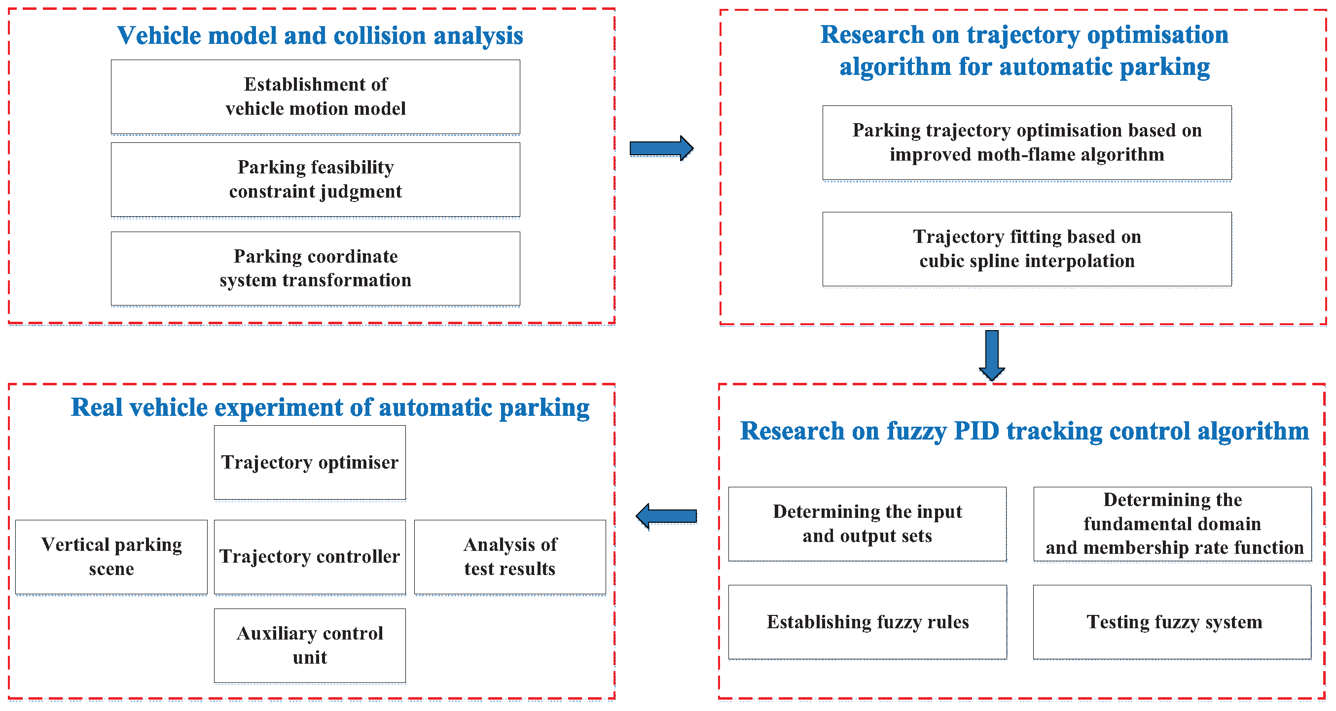
The parking behavior of automatically maneuvering vehicles that meets the parking eligibility criteria from the initiating region to the designated parking area is termed as ARP. Figure 1 illustrates the technical framework for this study.

In the form of ARP, the vehicle that meets the parking conditions in the garage is parked from the initiating region to the permitted parking region. The specific principal schematic principal diagram of ARP is as follows in Figure 2.

In Figure 2, we assume that during the ARP process, the region by vehicle body coverage is systematically collected in a sequential order $ns$ times, which is recorded as the set of fixed-point regions $(A_1,\dots ,A_{is},\dots ,A_{ns})$. Obviously, $A_1$ should be the initiating region, $A_{ns}$ should be the parking region, and $P_1$, $P_{is}$, and $P_{ns}$ are the center points of the fixed-point region, respectively. $L_b$ is the line of garage bottom, $L_{ne}$ and $L_{fe}$ are the near and far boundary lines of the parking garage, respectively, and $P_{nt}$, $P_{ft}$, $P_{nb}$, and $P_{fb}$ are the near corner and far corner of the garage top, near corner and far corner of the garage bottom, respectively. $T_R$ represents the reference trajectory for parking, while $T_C$ denotes the actual trajectory achieved through tracking control [19].

2.2. Feasibility Constraints Judgment for ARP

ARP is usually required to meet the following conditions: the location of the parking garage must be known, the boundary lines and corner points of the garage should be distinctly discernible, and there are no obstacles inside the parking garage [20]. In addition, it is necessary to meet the feasibility constraints of the parking garage: the central point $P_1$ of the parking initiating region should be in the permitted parking region ${\Omega }_{C,1}$. The line segment connecting the central point $P_1$ and the bottom midpoint $P_{b1}$ of the initiating region is $L_b$, and the angle between the line $L_b$ and the line $L_d$ of the garage bottom is defined as the initiating tilt angle $\Delta {\angle }_B$, with its absolute value being less than the threshold value $\Delta {\angle }_{Bmax}$. The constraint equation that determines the feasibility of initiating the parking process in the garage is outlined as follows:

$$\begin{array}{c}\hfill \begin{array}{c}\forall P_1\in {\Omega }_{C,1}\hfill \\ \left|{\angle }_B\right|=\left|\angle \left(T\left(P_1,P_{b1}\right),L_d\right)\right|<\Delta {{\angle }_B}_{max}\hfill \end{array}\end{array}$$

(1)

According to the initiating feasibility limitations of the parking garage shown in Formula (1), the initiating tilt angle should be small enough.

2.3. Principles of ARP Coordinate System Conversion

During the automatic parking process, the raw sensor data and system calculations need to be effectively connected through coordinate system alignment. Although the real-world coordinate system constructed from sensor data contains complete parking scene information, it suffers from baseline shift due to differences in sensor installation posture and distortion effects. Therefore, it needs to be converted into a unified standardized coordinate system: Taking the far corner of the parking space as the coordinate origin, extending the x-axis along the bottom line of the parking space, and determining the y-axis through the right-hand rule. This standardized system eliminates sensor deviations through the following three steps (scene extraction, coordinate system rotation, and origin translation), not only establishing a unified spatial reference for multi-source data but also significantly improving the computational efficiency of parking trajectory planning and tracking control. Additionally, it provides a coordinate reference that aligns with human spatial cognition for the visualization interface.

In the standardized Cartesian coordinate system for inbound parking planes, the coordinates of a point are determined to be $\left(x_s,y_s\right)$. It is straightforward to derive the angle $\angle B=arcsin\left({\displaystyle \frac{y_s}{\sqrt{{x_s}^2+{y_s}^2}}}\right)$ between this point and the x-axis.

$$\begin{array}{c}\hfill \begin{array}{c}{x}_r=\sqrt{{x_s}^2+{y_s}^2}·cos\left(\angle B-\angle A\right)+xf\hfill \\ y_r=\sqrt{{x_s}^2+{y_s}^2}·sin\left(\angle B-\angle A\right)+y_f\hfill \end{array}\end{array}$$

(2)

To further obtain the coordinates $\left(x_r,y_r\right)$ of this point in the real-world coordinate system, the real-world projection rotation angle $\angle A$ detected by the sensor system and the coordinates $\left(x_r,y_r\right)$ of the far corner point of the garage bottom in the real-world coordinate system can be substituted in the above reverse-engineer equation.

The real-world coordinates $\left(x_r,y_r\right)$ of this point can be obtained from the above reverse-engineer equation. To further obtain the conversion formula from $\left(x_r,y_r\right)$ to $\left(x_s,y_s\right)$, the real-world projection rotation angle $\angle A$ detected by the sensor system and the coordinates $\left(x_f,y_f\right)$ of the far corner point of the garage bottom in the real-world coordinate system can be substituted in the above reverse-engineer equation.

2.4. Optimization Model for Generating the Reference Trajectory in ARP

The parking process cycle is denoted as $\Delta t$, and the detailed optimization model for generating the reference trajectory in ARP is presented below:

$$\begin{array}{c}\hfill minL\left(T_R\right)={\int }_0^{T_{max}}v\left(t\right)dt\approx \sum _{it=1}^{nt}\Delta L_{it}\end{array}$$

(3)

$$\begin{array}{c}\hfill S.T.\left\{\begin{array}{c}\Delta L_{it}\le \Delta L_{max}\hfill \\ \Delta {\angle }_{it}\le \Delta {\angle }_{max}\hfill \\ \forall P_{is}\in {\Omega }_{C,is}\hfill \\ \forall P_g\left(ig\right)\notin {\Omega }_{c,it}\hfill \\ \forall P_g\left(ig\right)\in {\Omega }_g\hfill \\ \left|\Delta y_{ns}\right|=\left|y\left(P_{ns}\right)-y_H\right|\le \Delta {y_H}_{max}\hfill \end{array}\right.\end{array}$$

(4)

where, ${\Omega }_g$ is the coverage region of both boundary lines of the garage, and $P_g$ is the set of the boundary line collision-avoidance detection location points. $P_g\left(ig\right)$ is the $ig$-th boundary line collision-avoidance detection location point, $ig\in \left\{1,2,\dots ,ng\right\}$, $ng$ is the number of detection location points, obviously $\forall P_g\left(ig\right)\in {\Omega }_g$. $\Delta L_{it}$, $\Delta {\angle }_{it}$, and ${\Omega }_{c,it}$ are the parking interval distance, attitude angle difference, and region by vehicle body coverage in the $it$-th cycle. $\Delta L_{max}$ represents the threshold for parking interval distance, and $\Delta {\angle }_{max}$ is the threshold for the difference in attitude angle. $T_{max}$ represents the duration of parking, while $nt$ denotes the total number of cycles, $nt=⌈{\displaystyle \frac{T_{max}}{\Delta t}}⌉$, $it\in \left\{1,2,\dots ,nt\right\}$, and $\lceil \rceil$ is the carry up integer operator. During parking maneuvers, all collision detection points must stay outside the vehicle’s coverage area to avoid garage boundary collisions. That is, $\forall P_g\left(i\right)\notin {\Omega }_{c,it}$. Point $P_{is}$ represents the central location of the $is$-th fixed-point region, $is\in \left\{2,\dots ,ns\right\}$, while region ${\Omega }_{C,is}$ denotes its corresponding adjustable region, and so $\forall P_{is}\in {\Omega }_{C,is}$. The variable $\Delta y_{ns}$ signifies the error in parking position, $\Delta {y_H}_{max}$ indicates the threshold for the absolute value of this error, and $\Delta {y_H}_{max}$ corresponds to the ordinate value of the anticipated parking position. Trajectory $T_R$ serves as the reference path for parking, with its length $L\left(T_R\right)$ being key indicators that substantially influence the quality of parking optimization [21].

Consider an interval $\Delta =\left[a,b\right]$ with $n+1$ interpolation points $(x_0,x_1,\dots ,x_n)$ defined within this range, and the cubic spline interpolation function $s\left(x\right)$ is characterized by the following two properties.

The cubic spline function has two key advantages. First, the function is described by a cubic polynomial in each subinterval, implying that adjustments to a particular subinterval do not affect other subintervals. This locality facilitates the achievement of rapid outcomes when optimizing or adjusting the coordinates of specific region central points, without the need for recalculating the entire trajectory. Then, the cubic spline function is twice continuously differentiable over its entire domain, ensuring the smoothness of curvature variation along the trajectory. This high-order continuity enables the generation of exceptionally smooth curves. Based on these properties, applying cubic spline theory to handle the set of fixed-region centroids enables the quick generation of smooth parking reference trajectories, superior in both aspects to the geometric programming method [22].

Assuming that the center points’ coordinates of all fixed-point regions within the standardized parking plane system have been acquired, smooth parking reference trajectories can be rapidly generated by cubic spline interpolation fitting. This exhibits a notable advantage over geometric methods.

The algorithm in this study realizes the steering control of the vehicle based on the vehicle kinematics model. The so-called vehicle kinematics model refers to the following:

$$\begin{array}{c}\hfill \left\{\begin{array}{c}\dot{x}\left(t\right)=v\left(t\right)cos\left(\theta \left(t\right)\right)\hfill \\ \dot{y}\left(t\right)=v\left(t\right)sin\left(\theta \left(t\right)\right)\hfill \\ \dot{\theta }\left(t\right)={\displaystyle \frac{v\left(t\right)tan\left(\varphi \right(t\left)\right)}{l}}\hfill \\ \dot{v}\left(t\right)=a\left(t\right)\hfill \\ \dot{\varphi }\left(t\right)=w\left(t\right)\hfill \end{array}\right.\end{array}$$

(5)

where $(x,y)$ represents the center of the rear axle; v and a denote the velocity and acceleration of the vehicle, respectively; $\theta$ is the heading angle; $\varphi$ is the steering wheel angle; w is the steering wheel angular velocity; l is the length between the front and rear wheels, and t signifies time. $\dot{\theta }\left(t\right)={\displaystyle \frac{v\left(t\right)tan\left(\varphi \right(t\left)\right)}{l}}$ establishes the dynamic relationship between the steering angle $\varphi \left(t\right)$ and the change in the heading angle $\theta \left(t\right)$. The steering angle $\varphi \left(t\right)$ directly controls the rate of change of the vehicle’s heading angle $\theta \left(t\right)$.

To ensure that the trajectory generated during the vehicle’s steering process complies with the mechanical limitations of the vehicle’s steering mechanism, and at the same time meets the steering system’s requirement for continuous changes in the steering wheel angle, the following constraints are added:

$$\begin{array}{c}\hfill \left\{\begin{array}{c}\varphi \left(t\right)\in [{\varphi }_{min},{\varphi }_{max}]\hfill \\ |\dot{k}\left(t\right)|\le {\dot{k}}_{\max }\hfill \end{array}\right.\end{array}$$

(6)

where $\dot{k}={\displaystyle \frac{w\left(t\right)}{l{cos}^2\varphi }}$ represents the derivative of the instantaneous curvature.

3. Gene Modification of ARP

3.1. Basic Principles and Application Methods of Gene Modification

For diseased individuals, a targeted approach is employed to modify the defective gene segment, so that it makes correctly expressed genes alter their behavior. This process is referred to as gene modification. Traditional optimization algorithms typically eliminate all infeasible solutions generated during the optimization process (i.e., solutions that do not meet the constraints, also referred to as invalid solutions), and these approaches are not conducive to the preservation of optimization information. However, if some infeasible solutions are retained, the optimization efficiency will be adversely affected, while appropriate application of gene modification techniques will contribute to enhancing the preservation effect of optimized information. Considering both the calculation efficiency and increasing the number of parameters, this study modifies the far boundary line of the collision-avoidance garage and berthing tilt during the optimization of parking reference trajectory, and adopts new solutions to replace the other cases, which is an effective way to deal with the infeasible solutions of parking into a garage.

3.2. Gene Modification of Far Boundary Line for Collision-Avoidance Garage

In the standardized ARP coordinate system, the near boundary line of the garage corresponds to the vertical axis (y-axis). If the vehicle collides with the far boundary line of the garage during the $IT$-th cycle of the parking process, the bottom corner point $\left({x_{lb,}}_{IT},{y_{lb,}}_{IT}\right)$ on the left boundary of the vehicle must cross the far boundary line for the garage at this time. That is, its abscissa is less than 0. To modify the far boundary line of the collision-avoidance garage, the center point of the fixed-point region, which is located within a specified distance from the vehicle’s center, should be rotated counterclockwise to a certain extent.The empirical formula for determining whether the center point of the $is$-th fixed-point region rotates counterclockwise is presented as follows:

$$\begin{array}{c}\hfill \left|y\left(P_{is}\right)-y\left(tPget\left({x_{lb,}}_{IT},{y_{lb,}}_{IT}\right)\right)\right|\le \Delta Y_{fc,max}\end{array}$$

(7)

where $tPget\left({x_{lb,}}_{IT},{y_{lb,}}_{IT}\right)$ represents the function that determines the left corner at the bottom $\left({x_{lb,}}_{IT},{y_{lb,}}_{IT}\right)$ corresponding to the vehicle’s center, and $\Delta Y_{fc,max}$ denotes the greatest permissible deviation along the vertical axis.

If the above formula is true, then the specified $is$-th fixed-point region central point rotates counterclockwise accordingly, and the empirical formula of the abscission offset $\Delta x_{is,fc}$, modifying the far boundary line for the collision-avoidance garage, is presented below:

$$\begin{array}{c}\hfill \Delta x_{is,fc}=\left(x\left(tPget\left({x_{lb,}}_{IT},{y_{lb,}}_{IT}\right)\right)-x\left(P_{is}\right)\right)·c_{fc}·{x_{lb,}}_{IT}\end{array}$$

(8)

where $c_{fc}$ is the empirically determined coefficient value of the far boundary line for the collision-avoidance garage.

The specific gene modification schematic diagram on the far boundary line is displayed in Figure 3.

In Figure 3, $\left(x_{fc},y_{fc}\right)$ represents the vehicle’s center of the boundary crossing point of the far boundary line for the collision-avoidance garage during the parking process. The abscissa of the center points $P_{is1}$, $P_{is2}$, and $P_{is3}$ of the fixed-point region in the interval $\left(y_{fc}-\Delta Y_{fc,max},y_{fc}+\Delta Y_{fc,max}\right)$ are adjusted by distances $\Delta x_{is-1,fc}$, $\Delta x_{is-2,fc}$, and $\Delta x_{is-3,fc}$, respectively, thus achieving the purpose of modifying the far boundary line for the collision-avoidance garage.

3.3. Berthing Tilt Gene Modification

If the absolute value of the berthing tilt angle $\Delta {\angle }_S$ surpasses the specified threshold $\Delta {\angle }_{S max}$, that is, $\left|\Delta {\angle }_S\right|>\Delta {\angle }_{S max}$, this condition is defined as berthing tilt. To modify the berthing tilt, it is necessary to appropriately shift the central points’ x coordinate within the fixed-point region to the right. Based on experience, the decision formula for determining the rightward shift of the center points’ abscissa of the $is$-th fixed-point region is presented below:

$$\begin{array}{c}\hfill y\left(P_{is}\right)-y\left(P_{ns}\right)\le \Delta Y_{SI,max}\end{array}$$

(9)

where $\Delta Y_{SI,max}$ represents the maximum vertical axis offset for modifying the berthing tilt.

If the above formula is true, the center points’ abscissa of the $is$-th fixed-point region should be appropriately shifted to the right. The specific empirical formula for the rightward abscissa movement $\Delta x_{is,SI}$ of the modifying berthing tilt is outlined below:

$$\begin{array}{c}\hfill \Delta x_{is,SI}=\left(y\left(P_{is}\right)-y\left(P_{ns}\right)\right)·tan(\Delta {\angle }_S-\Delta {\angle }_{S max})\end{array}$$

(10)

The specific gene modification schematic diagram related to berthing tilt is presented in Figure 4.

The central points’ abscissa $P_{ns-1}$ and $P_{ns-2}$ of the fixed-point region in the interval $\left(y_{ns},y_{ns}+\Delta Y_{SI,max}\right)$ are adjusted to the right by distances $\Delta x_{ns-1,SI}$ and $\Delta x_{ns-2,SI}$, respectively, thus realizing the purpose of modifying the berthing tilt.

4. Description of IDMMFO-GM Design

4.1. Introduction to the MFO Algorithm

The MFO algorithm is a swarm intelligence algorithm that was introduced in 2015. This algorithm abstracts the moth’s navigation toward a light source by employing lateral positioning strategies to develop an optimization approach. The MFO algorithm has two important elements: the moth and the flame. The moth is the actual individual in the optimization process, which stands for candidate solution, while the flame symbolizes the optimal solution identified by the moth through the last iteration.

Matrix M exhibits the location for the moth population:

$$\begin{array}{c}\hfill M=\left[\begin{array}{cccc}{M}_{11}& M_{12}& \dots & M_{1d}\\ M_{21}& M_{22}& \dots & M_{2d}\\ ⋮& ⋮& ⋮& ⋮\\ M_{n1}& M_{n2}& \dots & M_{nd}\end{array}\right]\end{array}$$

(11)

where n denotes the overall count of moth individuals, and d represents the dimensionality of the solution domain.

The fitness values for the moth population are encapsulated in the matrix $OM$:

$$\begin{array}{c}\hfill OM=\left[\begin{array}{c}O{M}_1\\ O{M}_2\\ ⋮\\ O{M}_n\end{array}\right]\end{array}$$

(12)

During the preliminary phase of the algorithm’s iteration process, total flame amount is equivalent to the total number of moth individuals. The initial location of the flame set is denoted through matrix F:

$$\begin{array}{c}\hfill F=\left[\begin{array}{cccc}{F}_{11}& F_{12}& \dots & F_{1d}\\ F_{21}& F_{22}& \dots & F_{2d}\\ ⋮& ⋮& ⋮& ⋮\\ F_{n1}& F_{n2}& \dots & F_{nd}\end{array}\right]\end{array}$$

(13)

The fitness value for flame set is denoted through matrix $OF$:

$$\begin{array}{c}\hfill OF=\left[\begin{array}{c}O{F}_1\\ O{F}_2\\ ⋮\\ O{F}_n\end{array}\right]\end{array}$$

(14)

The optimization procedure of the MFO algorithm is summarized by a triplet:

$$\begin{array}{c}\hfill MFO=(I,P)\end{array}$$

(15)

I denotes the algorithm’s initiating operation, which is mainly shown as follows: randomly generating individual moths within the solution domain and subsequently obtaining their respective fitness values.

The association rule for this process is formulated as described below:

$$\begin{array}{c}\hfill I:\varphi \to \left\{M,OM\right\}\end{array}$$

(16)

P denotes the principal function that guides the moth’s trajectory update once the optimization algorithm initiates its operation. Specifically, the moth adjusts its location according to its own information and that of the flame set, following the logarithmic helical law, and subsequently computes the fitness value of the updated location. If this value surpasses the fitness value of the corresponding flame, the flame’s location is updated accordingly.

The mapping relationship for this process can be described as follows:

$$\begin{array}{c}\hfill P:M\to M\end{array}$$

(17)

T represents the logarithmic helical location adjusting behavior of individual moths. The moth is updated by the logarithmic helical rule as follows:

$$\begin{array}{c}\hfill \left\{\begin{array}{c}{M}_i=S(M_i,F_j)=D_{ij}·e^{\tau t}·cos\left(2\pi t\right)+F_j\hfill \\ D_{ij}=|M_i-F_j|\hfill \end{array}\right.\end{array}$$

(18)

where $M_i$ denotes the location of the i-th moth, $F_j$ denotes the location of the j-th flame, $D_{ij}$ signifies the Euclidean distance location from the i-th moth to the j-th flame, $\tau$ is the variable of altering the location logarithmic helical waveform, t is a stochastic value within the range of −1 to 1, and $S(M_i,F_j)$ also signifies the logarithmic helical function.

Furthermore, with the rate of algorithm convergence, the quantity of flames will dynamically diminish as the number of iterations increases. The adaptive adjustment mechanism for the flame count is outlined below:

$$\begin{array}{c}\hfill N_{flame}=round(N_{flame}^{max}-l{\displaystyle \frac{N_{flame}^{max}-1}{N_{\mathrm{int}}^{max}}})\end{array}$$

(19)

where $N_{flame}$ represents the number of flames after updating, l indicates the present iteration count, $N_{flame}^{max}$ denotes the maximum count of flames, and $N_{\mathrm{int}}^{max}$ signifies the upper limit of iterations allowed.

4.2. Non-Linear Decreasing Strategy of Weight Coefficient

To achieve a more effective balance between global and local searching, a non-linear decreasing approach for the weight coefficient associated with the logarithmic helical term is introduced in this study. This approach aims to address the inherent limitation of the moth–flame optimization, which is prone to converging prematurely to local optima. The specific mapping expression for the logarithmic helical location adjusting behavior of the moth individual is as follows:

$$\begin{array}{c}\hfill T:\left\{\begin{array}{c}{M}_i=\omega ·D_{ij}·e^{\tau t}·cos\left(2\pi t\right)+F_j\hfill \\ D_{ij}=|M_i-F_j|\hfill \end{array}\right.\end{array}$$

(20)

When the weight coefficient $\omega$ is higher, the algorithm exhibits significant global searching performance, which is particularly appropriate for the preliminary phase of the optimization procedure. Conversely, when the weight coefficient $\omega$ is lower, the algorithm demonstrates enhanced local searching. In this study, we propose a non-linear decreasing approach about the flexible weight coefficient $\omega$ and propose it relying on the cosine structure.

The specific non-linear decreasing function about the weight coefficient $\omega$ of iteration progress $t_r$ is presented in Figure 5.

The specific formula for calculating the weight coefficient $\omega$ is presented as follows:

$$\begin{array}{c}\hfill \omega ={\omega }_{min}+{\omega }_d·cos{\left(\left(1-t_r\right)·{\displaystyle \frac{\pi }{2}}\right)}^{\beta }\end{array}$$

(21)

where ${\omega }_d$ represents the weight coefficient decrement, ${\omega }_d={\omega }_{max}-{\omega }_{min}$, and ${\omega }_{min}$ and ${\omega }_{max}$ denote the lower and upper limits of the weight coefficients, respectively. $t_r$ signifies the progression of the iteration, $t_r=t·{t_{max}}^{-1}$, and $\beta$ is the optimization factor for the non-linear decreasing about the weight coefficient $\omega$.

As illustrated in Figure 5, the cosine structure non-linear decreasing strategy exhibits significant adaptability and flexibility. Specifically, this strategy is employed to optimize and adjust the weight coefficient by selecting the most appropriate optimization parameter; hence, it enables real-time adjustment of the weight coefficient decreasing rate during the iterative process, which is conducive to the improvement in the balance effect between global exploration and local development, to improve the overall optimization ability of the algorithm [23].

4.3. Directional Mutation Strategy

At the end of the optimization of the MFO algorithm, the moth population is easily affected by the flame set, thus leading a high risk of local convergence. By introducing the mutation operator of the genetic mechanism, the diversity of the moth population can be significantly enhanced, to reduce the risk of the algorithm falling into local convergence. Compared with traditional random mutation based on a certain mutation probability, directional mutation guided by gradient information significantly enhances the convergence speed and optimization precision of the algorithm.

The specific process of directional mutation in parking reference trajectory optimization is outlined as follows:

Parking reference trajectory optimization is a specific type of optimization problem aimed at minimizing a single objective. Generally, this class’s problems can be formally described as follows:

$$\begin{array}{c}\hfill miny=F\left(u\right)\end{array}$$

(22)

where y represents the optimization objective, u denotes the decision variable, and $F\left(u\right)$ signifies the optimization mapping model for solving the optimization objective y of decision variable u. For the parking reference trajectory optimization problem, the decision variable u is defined as the center point set $PS$ of the fixed-point region to be decided, $PS=\left\{P_2,\dots ,P_{ns}\right\}$, while the objective function $F\left(u\right)$ represents the length $L\left(tf\left(PS\right)\right)$ of the reference trajectory.

The original decision variable to be directed mutation is denoted as $P{S}_k$, the gene inheritance decision variable for directional mutation is denoted as $P{S}_i$, and the gene changing decision variable for directional mutation is denoted as $P{S}_j$. Subsequently, the directed vector $d\left(P{S}_j,P{S}_i\right)$ can be formally defined as follows:

$$\begin{array}{c}\hfill d\left(P{S}_j,P{S}_i\right)=\mathrm{sgn}\left(\left\{P_{2,j}-P_{2,i},\dots ,P_{ns,j}-P_{ns,i}\right\}\right)\end{array}$$

(23)

where $\mathrm{sgn}$ represents a symbolic function that denotes the sign of the parameters, including 0, −1, and 1.

If $L\left(tf\left(P{S}_j\right)\right)<L\left(tf\left(P{S}_i\right)\right)$, the vector $d\left(P{S}_i,P{S}_j\right)$ represents the evolutionary direction of objective function $L\left(tf\left(PS\right)\right)$ from the gene inheritance decision variable $P{S}_i$ to the gene changing decision variable $P{S}_j$. Conversely, the vector $d\left(P{S}_i,P{S}_j\right)$ denotes its degenerate direction. Gene inheritance decision variable $P{S}_i$ usually selects the original decision variable $P{S}_k$ or its direct parent, while selecting the gene changing decision variable, it should be chosen to be as far as possible from the original decision variable $P{S}_k$.

Through the application of direction vector $d\left(P{S}_j,P{S}_i\right)$, the directional mutation of the original decision variable $P{S}_i$ can be carried out. The specific formulation is as follows:

$$\begin{array}{c}\hfill P{S_k}^{\prime }=P{S}_i+{\omega }_m·r·d\left(P{S}_j,P{S}_i\right)\end{array}$$

(24)

where $P{S_i}^{\prime }$ represents the original decision variable to be directed mutation, $P{S}_k$ denotes the updated decision variable after directional mutation, and ${\omega }_m$ signifies the adjustment coefficient for directional mutation, ${\omega }_m\in \left(0,1\right)$.

It is assumed that at the i-th iteration, the i-th moth $M_{t,i}$ in the current moth population $M_{t,i}$ is to be directed mutation, and it is taken as the gene inheritance decision variable, and the j-th flame ${F_{t,}}_j$ in flame set $F_t$ is randomly selected as the gene changing decision variable of its directional mutation. The gene inheritance decision variable determined by moth $M_{t,i}$ is denoted as $P{S}_i$, while the gene changing decision variable determined by flame ${F_{t,}}_j$ is represented as $P{S}_j$. The fitness values of moth and flame are denoted as $L\left(tf\left(P{S}_i\right)\right)$ and $L\left(tf\left(P{S}_j\right)\right)$, respectively, and directional mutation can be achieved.

According to the above formulas, by regulating the directional mutation adjustment coefficient ${\omega }_m$, the global and local exploration of the algorithm can be more effectively balanced, to promote the whole effect of the algorithm.

Specifically, the flowchart for IDMMFO proposed in this study is shown in Figure 6.

5. Test Verification

5.1. Description of the Test Scene for ARP

In this study, the ARP scene of space No.155 in the garage of Dalian Shell Museum, which is situated within Dalian Xinghai Square, was selected as the actual parking test site. The lengths of the near boundary and far boundary lines for the test garage were identical, both of which were 5 m in length. To carry out engineering validation of the IDMMFO-GM strategy introduced in this study, a series of actual vehicle tests were performed using a designated test vehicle. The test vehicle model was the Toyota Corolla 1.2T S-CVT GL Pioneer Edition (2019 model year), measuring 4635 mm in length, 1780 mm in width, and 1455 mm in height. This vehicle was equipped with an ETRS electronic transmission system and an EPS electric power steering system, thus enabling automated control of steering, acceleration, braking, and gear shifting. The distances along the horizontal and vertical, measured from the bottom right corner of the test vehicle’s initiating region to the nearby top corner of the parking garage, were 2.0 m and 2.1 m, respectively.

5.2. Development and Settings of ARP Test

This study employed a test vehicle outfitted with the ARP system, incorporating a real-time MPC555LFMZP40 trajectory optimizer and trajectory controller chip, as well as a DSP28335 auxiliary control unit and data awareness system. Additionally, the system included an execution drive unit chip and various essential actuators. The data awareness system mainly comprised a surround-view camera for detecting parking garage information, a radar for obstacle avoidance, and a camera controller for analyzing the data collected by the surround-view camera. Additionally, the system included an execution drive unit chip and various essential actuators. During the ARP process, the vehicle’s driver monitored real-time braking status via the ARP monitoring upper computer without interfering with the normal ARP operations. Only when necessary, the driver can apply the braking instruction or emergency braking parking instruction to make the test vehicle park or for emergency braking. The overall design diagram of the ARP test is displayed in Figure 7.

The main settings for the ARP test adopted in this study are outlined as follows: data acquisition for braking, assessment of parking feasibility, optimization of reference trajectory, tracking control of reference trajectory, emergency braking, and braking time limits. The limit time of each process was 3.5 s, 1.5 s, 10 s, 25 s, 0.4 s, and 1.5 s, respectively. At least one ARP driver holding a C2 driving qualification in the vehicle, one external safety inspector, and one skilled unmanned aerial photographer should be equipped; the unmanned aerial camera used was the DJI “Royal” Mavic 2; the ARP monitoring host computer was configured with a “MacBook Pro 2016 Core i5 @ 2.9 GHz”; and the communication was carried out by Bluetooth on board.

The ARP procedure integrates five stages: environmental sensing, feasibility assessment, trajectory optimization, fuzzy PID control, and emergency braking. Radar and Around View Monitor (AVM) data fusion ensured stability in complex scenarios. The data awareness system of the test vehicle utilized multi-sensor fusion technology, and it mainly comprises a surround-view camera for detecting parking garage information, radar for obstacle avoidance, and a camera controller for analyzing the data collected by the surround-view camera. The data awareness system is composed of a ring array of 12 ranging radars and an AVM system equipped with four high-precision cameras. Specifically, eight radars are positioned on the sides of the front and rear bumpers, while the other four are mounted on the front bumper; the radar array precisely identifies obstacles and delineates parking space contours via a comprehensive ${360}^{°}$ monitoring network. The AVM system employed wide-angle cameras located at the bottom of the front grille, license plate lights, and rearview mirrors to capture images, which were subsequently transmitted via CVDS or LVDS. It then produced a switchable 2D/3D panoramic view without black edges by applying fisheye correction and multi-perspective stitching techniques. The system’s design incorporates an overlapping field of view and a dynamic compensation mechanism, which can tolerate up to a $1^{°}$ assembly error. Additionally, an automatic rotation mechanism is employed to address image offset caused by vehicle vibrations.

5.3. Test Results and Comparative Analysis from ARP

Based on an actual ARP scene, this study employed four advanced optimization algorithms to refine the parking reference trajectory for improved performance. Specifically, the following algorithms were applied: the improved directional mutation moth–flame algorithm via gene modification (IDMMO-GM) proposed in this study, an enhanced immune MFO algorithm according to gene correction (IIMFO-GC) [24], an improved particle swarm optimization algorithm (IPSO) [20], and an enhanced immune shark smell optimization algorithm (IISSO) [21]. Additionally, these algorithms uniformly employed fuzzy proportional–integral–derivative (PID) control to achieve precise reference trajectory tracking. To ensure an impartial comparison, the ARP reference trajectory optimization model utilizing the aforementioned algorithms all employed identical parameter settings, as detailed in

Table 2. Parameter settings for ARP trajectory optimization model.

Name	Symbol	Value
Initiating tilt angle threshold	$\Delta {\angle }_{B max}$	${\displaystyle \frac{\pi }{75}}$
Center point number	$ns$	10
Parking tilt angle threshold	$\Delta {\angle }_{S max}$	${\displaystyle \frac{\pi }{75}}$
Parking location error threshold	$\Delta y_{ns}$	$0.15$ m
Parking process cycle	$\Delta t$	$1500\mathsf{\mu }$s
Attitude angle difference threshold	$\Delta L_{max}$	$5·{10}^{-4}\pi$
Parking interval threshold	$\Delta {\angle }_{max}$	${10}^{-3}$ m

. The parameter settings for IDMMFO-GM applied in the ARP reference trajectory optimization model are presented in

Table 3. Parameter settings of IDMMFO-GM algorithm for ARP reference trajectory optimization model.

Name	Symbol	Value
Moth population size	n	30
Iteration number	$t_{max}$	80
Logarithmic helical waveform adjustment coefficient	$\tau$	1
Minimum weight coefficient	${\omega }_{min}$	$0.3$
Maximum weight coefficient	${\omega }_{min}$	$0.9$
Non-linear decreasing optimization factor	$\beta$	$1.85$
Directional mutation adjustment coefficient	${\omega }_m$	$0.66$
Maximum vertical axis offset for collision-correction garage	$\Delta Y_{fc,max}$	$0.92$ m
Abscissa moving to the right empirical coefficient	$c_{fc}$	$0.58$
Maximum vertical axis offset of modification berthing tilt	$\Delta Y_{SI,max}$	$0.84$ m

.

To achieve a fair comparison of the four optimization algorithm, three designated fixed-point regions ($A_{10}$, $A_7$, $A_4$) were selected, where $y\left(P_{10}\right)\in \left[2.35,2.40\right]$, $y\left(P_7\right)\in \left[4.55,4.65\right]$, and $y\left(P_4\right)\in \left[6.10,6.25\right]$. The detailed results of ARP optimization and tracking control are presented in

Table 4. Berthing tilt angles for ARP trajectory optimization and tracking control.

Algorithms	Optimization	Tracking Control
IDMMFO-GM	0.43	0.48
IIMFO-GC	1.03	1.08
IISSO	3.83	3.90
IPSO	1.70	1.77

,

Table 5. Fixed-point regions’ positions and path lengths for ARP trajectory optimization.

Algorithms	Center Point Coordinates (m)	Path Length (m)
IDMMFO-GM	(1.56, 2.39), (1.57, 4.63), (1.92, 6.21)	9.435
IIMFO-GC	(1.44, 2.38), (1.47, 4.64), (1.81, 6.22)	9.483
IISSO	(1.18, 2.41), (1.43, 4.65), (1.72, 6.23)	9.693
IPSO	(1.10, 2.40), (1.22, 4.60), (1.56, 6.20)	9.768

,

Table 6. Fixed-point regions’ positions and path lengths for ARP trajectory tracking control.

Algorithms	Center Point Coordinates (m)	Path Length (m)
IDMMFO-GM	(1.50, 2.37), (1.51, 4.61), (1.86, 6.19)	9.456
IIMFO-GC	(1.38, 2.37), (1.39, 4.63), (1.75, 6.21)	9.508
IISSO	(1.21, 2.40), (1.42, 4.64), (1.85, 6.22)	9.617
IPSO	(1.22, 2.39), (1.28, 4.55), (1.62, 6.11)	9.647

and

Table 7. Comparison of parking time required by different algorithms.

Algorithms	Optimization Time Required (s)	Tracking Control Time (s)
IDMMFO-GM	9.02	18.79
IIMFO-GC	9.41	19.60
IISSO	9.57	19.94
IPSO	9.68	20.17

. The specific optimization trajectories and tracking control curves for the ARP system, as monitored by the host computer, are depicted in Figure 8 and Figure 9. The designated fixed-point regions’ curves for ARP trajectory optimization and tracking control, as determined by the host computer monitoring, are presented in Figure 10 and Figure 11. An actual unmanned aerial image of the fixed-point regions for ARP trajectory tracking control is shown in Figure 12.

As illustrated in Figure 8, compared with the three optimization algorithms used for comparison, IDMMFO-GM shows superior optimization performance in obtaining an ideal reference trajectory, and it exhibits a shorter path length and a smaller expected berthing tilt angle in its reference trajectory. As depicted in Figure 9, the IDMMFO-GM algorithm demonstrates higher tracking control performance when employing the fuzzy PID tracking algorithm. Consequently, the resulting trajectory exhibits a reduced path length and a smaller actual berthing tilt angle. As shown in Figure 10, compared with the three optimization algorithms used for comparison, the IDMMFO-GM algorithm exhibits better optimization performance in generating an optimal reference trajectory. The trajectory produced by IDMMFO-GM not only approaches the garage’s boundary line more closely but also results in a reduced expected berthing tilt angle. As displayed in Figure 11 and Figure 12, the IDMMFO-GM algorithm describes enhanced tracking control performance when using the fuzzy PID algorithm. The resulting trajectory is nearer to the garage’s boundary line and exhibits a smaller actual berthing tilt angle. In Figure 11, the IDMMFO-GM algorithm aligns the vehicle toward the right side of the parking garage. Specifically, the x-axis coordinate of the vehicle’s final parking position is greater compared to that achieved by other algorithms. Consequently, with the same initiating region, the IDMMFO-GM algorithm demands the least land area, significantly minimizing the construction and operational costs associated with parking facilities. On the other hand, a more to the right position results in a shorter path length. As the vehicle maintains an approximately steady speed while parking, this indicates that the vehicle will require less stopping time, thus enhancing the users’ overall experience.

Table 4 and Table 5 indicate that IDMMFO-GM surpasses the three comparative algorithms in both reference and actual trajectories. Specifically, it results in a reduced reference trajectory length. Moreover, when the fuzzy PID tracking algorithm is employed, it achieves a shorter actual trajectory length in tracking control. As presented in Table 6, compared with the three optimization algorithms used for comparison, IDMMFO-GM demonstrates a notably smaller expected berthing tilt angle in its reference trajectory. Furthermore, when employing the same tracking control algorithm (fuzzy PID), it achieves a significantly smaller actual berthing tilt angle in its actual trajectory. As illustrated in Table 7, in comparison with the other three algorithms, IDMMFO-GM exhibits a markedly shorter optimization time requirement. Moreover, when utilizing the same fuzzy PID control algorithm, it further attains a significantly reduced tracking control time.

5.4. Simulation Results and Comparative Analysis from ARP

To further validate the effectiveness of the proposed algorithm, simulation verification for ARP trajectory optimization and actual tracking control was conducted using the Matlab simulation platform. A monitoring platform based on Visual Studio was employed to monitor the entire ARP trajectory optimization process, with communication established using Visual C++ 6.0 and the communication medium being Office Excel. The simulation environment was configured as follows: Matlab version 2016b, Visual Studio version VS2015, computer processor model Core i7-9800X @ 3.80 GHz, and Office Excel version Office Excel 2017. The ARP-optimized trajectory model based on Matlab simulation and the key parameters of IDMMFO-GM are described in Table 2 and Table 3, respectively. The pchip function was utilized to construct the cubic spline interpolation function, while the integral fitting method was adopted to solve parking curve length calculations.

This study selected parking space No. 155 at Dalian Shell Museum in Xinghai Square, Dalian, as the test scenario for automatic parking. The lengths of both the near-side and far-side boundary lines of the test garage were measured as 5.0 m, while the length of the rear boundary line was recorded as 2.7 m, with the width of the parking space markings being 0.1 m. The test vehicle used was a Volkswagen Tiguan (2016 model, 1L variant), with its length, width, and height being specified as 3540 mm, 1645 mm, and 1509 mm, respectively. The initiating position of the vehicle was such that the horizontal distance between the bottom right corner of its coverage area and the far corner of the parking space was measured as 2.2 m, while the longitudinal distance was recorded as 1.0 m.

Under the aforementioned simulation conditions, comparative tests were conducted between the proposed IDMMFO-GM and three algorithms: IIMFO-GC, IISSO, and IPSO. The trajectory optimization simulation curves and related results are presented in Figure 13 and

Table 8. Fixed-point positions and path lengths for ARP trajectory optimization in Matlab simulation environment.

Algorithms	Center Point Coordinates (m)	Path Length (m)
IDMMFO-GM	(1.55, 2.44), (1.53, 3.84), (2.07, 6.01)	9.19
IIMFO-GC	(1.20, 2.45), (1.21, 3.95), (1.92, 6.15)	9.75
IISSO	(1.32, 2.49), (1.35, 3.86), (2.02, 6.15)	9.63
IPSO	(1.11, 2.45), (1.22, 3.93), (1.89, 6.15)	9.88

.

As illustrated in Figure 13 and Table 8, compared with IIMFO-GC, IISSO, and IPSO, the simulation-optimized trajectory obtained through IDMMFO-GM demonstrates a shorter berthing trajectory length, and closer proximity to the garage’s near-side boundary line. This indicates that the proposed IDMMFO-GM possesses superior optimization capabilities, enabling the identification of more desirable parking trajectories and achieving enhanced ARP trajectory optimization outcomes.

6. Conclusions

ARP systems have a broad spectrum of practical applications across various fields including commercial, civilian, military, and ceremonial domains. However, trajectory optimization for ARP systems presents a multi-objective, non-linear, and extremely difficult optimization challenge. Consequently, obtaining an ideal reference trajectory that makes its curve collision-avoidance smoothness and short path lengths, is particularly difficult. To effectively enhance the performance of ARP trajectory optimization, a gene modification optimization algorithm, IDMMFO-GM, is proposed in this study. In contrast to current research achievements on optimizing reference trajectories for automatic parking, the key contributions of this study can be summarized as follows:

A novel reference trajectory optimization model for ARP is developed. Integrating cubic spline interpolation with the standardized parking plane coordinate system, an effective and practical reference trajectory optimization framework is established, which takes into account the feasibility constraints of parking, including the initiating region and berthing tilt angle; hence, it can effectively describe and optimize ARP trajectory.

To address the issue of infeasible solutions and balance the algorithm’s global exploitation and local development capabilities, an IDMMFO-GM is introduced. This algorithm organically integrates the gene modification mechanism, the non-linear decreasing weight coefficient strategy, and the directional mutation strategy, which can effectively utilize infeasible solutions encountered during computation, thus improving its global optimization performance and avoiding local convergence.

While the IDMMFO-GM algorithm exhibits excellent performance in optimizing automatic parking trajectories, it still possesses certain constraints: (I) Concerning parameter sensitivity, the algorithm’s empirical coefficients require manual tuning. This not only raises deployment expenses but might also compromise the algorithm’s adaptability in parking scenes. To achieve dynamic parameter adjustment, the implementation of online calibration technology is essential. (II) Regarding the constraint of dynamic adaptability, the current research is primarily grounded in the static environment hypothesis and does not account for real-time interference factors such as pedestrian movement and dynamic obstacles. In future work, mechanisms for predicting and avoiding dynamic obstacles will be incorporated. (III) Considering the sensitivity of sensor errors, the precision of transforming into a standardized coordinate system largely relies on the quality of sensor calibration. This reliance becomes more significant under extreme conditions, such as low light or adverse weather like rain and snow, where error accumulation is more likely to occur. Therefore, adopting a multi-source sensor fusion approach is essential for enhancing the stability of the system. (IV) At the multi-objective optimization level, the current model focuses solely on path length as its optimization goal and does not adequately account for various factors, including the rate of change in steering angle and energy consumption efficiency. This could result in practical issues, such as decreased comfort during application. Moving forward, the integration of multi-objective optimization algorithms will aim to address and harmonize the diverse performance requirements across dimensions.

To validate the efficacy of the proposed IDMMFO-GM, an automatic parking test is conducted for verification. Actual vehicle tests show that IDMMFO-GM outperforms three high-performance comparative optimization algorithms in parking trajectory optimization. Additionally, its trajectory tracking control performance is markedly improved.