
A Simulation of Contact Graph Routing for Mars–Earth Data Communication


Abstract
1. Introduction
- Custody Transfer: A node takes responsibility for forwarding the bundle, improving delivery assurance.
- Late Binding: Enables routing decisions to be made later, once more info is available.
- Opportunistic Forwarding: Uses available contact plans or real-time link availability.
2. Model of CGR
- Arrangement of the contact graph: determination of the number of nodes being used, possible routing among n nodes, storage capacities of satellites, the observed time per minute in a Martian day, contact window schedule between rovers and satellites, and between satellites and DSN antennas.
- Arrangement of data: generating random data size per minute, distributing data into d packets whose maximum size is 256 Kbytes.
- Routing management for the combination of rover and satellite.
- Routing management for the combination of satellite and DSN antenna.
- Plotting the graph.
2.1. Arrangement of the Contact Graph
2.2. Arrangement of Data
2.3. Routing Management for the Combination of Rover and Satellite
- (i)
- The contact window between i and j is open, or ;
- (ii)
- for all w with , and the storage is not full;
- (iii)
- There is any DSN-antenna k, such that .
2.4. Routing Management for the Combination of Satellite and DSN Antennas
- and , so data are delivered smoothly from Mars to Earth in the same time.
- When there is only and there are data being stored at satellite j from the previous time interval(s).
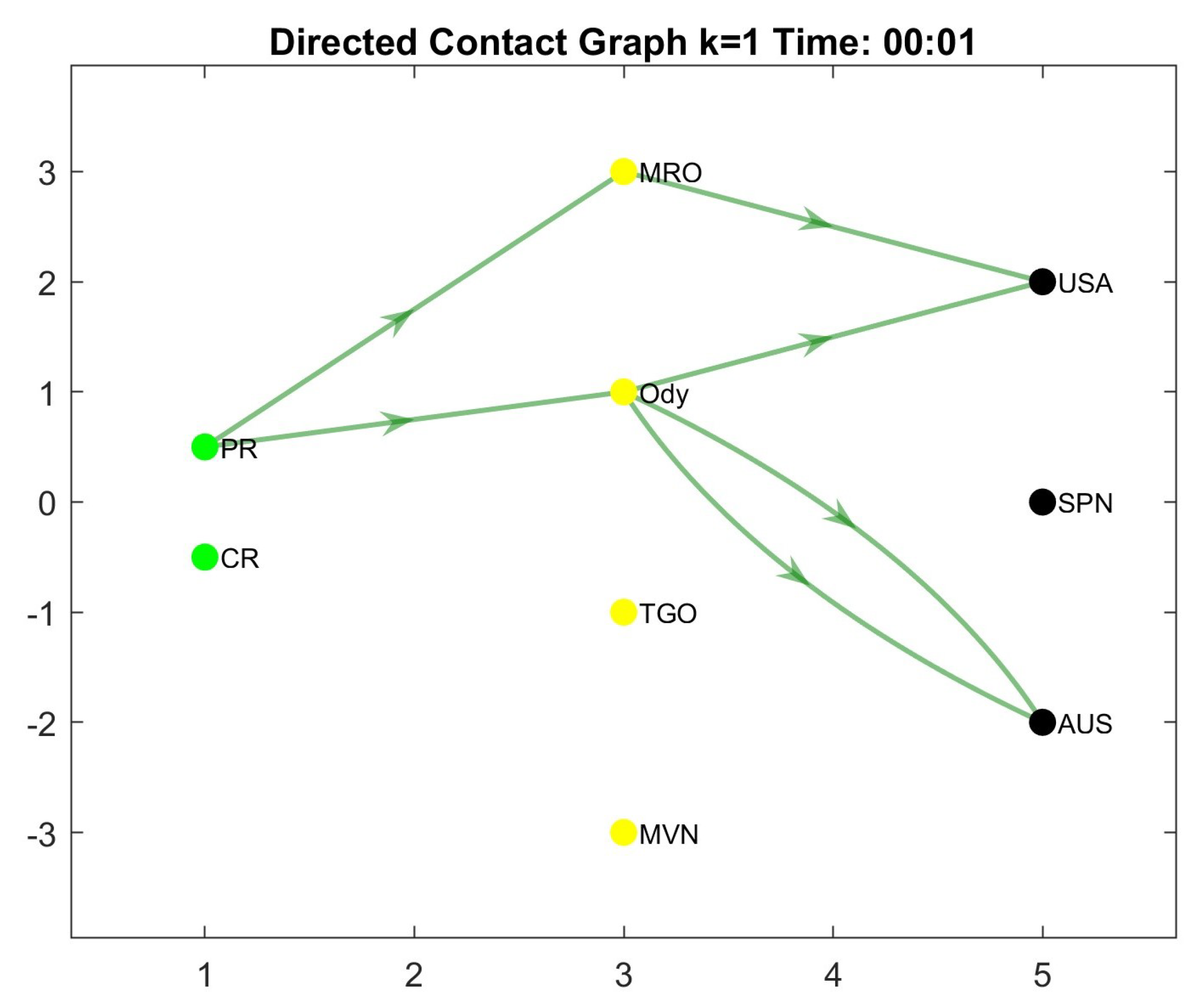
2.5. Plotting the Graph
- x means , and x means , so packet-1 is delivered in routes ;
- x means , and x means , so packet-2 is delivered in routes ;
- x means , so packet-3 is delivered in route ;
- x where , so packet-3 is delivered in route .
3. Algorithms of the Model
| Algorithm 1 Main Algorithm |
|
| Algorithm 2 Procedure RoverSatelliteRouting |
|
| Algorithm 3 Satellite–Antenna Routing |
|
4. Simulation Results and Discussion
5. Conclusions
Author Contributions
Funding
Data Availability Statement
Acknowledgments
Conflicts of Interest
References
- ESA. Why Go to Mars? 2019. The Eropean Space Agency. Available online: https://www.esa.int/ScienceExploration/HumanandRoboticExploration/Exploration/WhygotoMars (accessed on 1 December 2024).
- NASA. 2024. Available online: https://eyes.nasa.gov/apps/mrn/#/mars (accessed on 1 December 2024).
- Birrane, E.; Burleigh, S.; Kasch, N. Analysis of the contact graph routing algorithm: Bounding interplanetary paths. Acta Astronaut. 2012, 75, 108–119. [Google Scholar] [CrossRef]
- Herkenhoff, K. Sol 1128: Twenty Minutes to Mars. 2015. Available online: https://science.nasa.gov/blog/msl-update-2442/ (accessed on 1 December 2024).
- Kugler, L. Direct-Dialing Mars? 2024. Available online: https://cacm.acm.org/news/direct-dialing-mars/ (accessed on 1 December 2024).
- Ormston, T. Time Delay Between Mars and Earth. 2012. Available online: https://blogs.esa.int/mex/2012/08/05/time-delay-between-mars-and-earth/ (accessed on 1 December 2024).
- Benamar, N.; Singh, K.D.; Benamar, M.; El Ouadghiri, D.; Bonnin, J.M. Routing protocols in Vehicular Delay Tolerant Networks: A comprehensive survey. Comput. Commun. 2014, 48, 141–158. [Google Scholar] [CrossRef]
- Elewaily, D.I.; Ali, H.A.; Saleh, A.I.; Abdelsalam, M.M. Delay/Disruption-Tolerant Networking-based the Integrated Deep-Space Relay Network: State-of-the-Art. Ad. Hoc. Netw. 2024, 152, 103307. [Google Scholar] [CrossRef]
- NASA. Mars Exploration Program Mars Relay Description for Discovery 2019 Proposals. 2019. Available online: https://discovery.larc.nasa.gov/PDF_FILES/21_Proposers_Guide_To_Mars_Orbiters_-_Discovery_2019_AO_-_Rev_190411b.pdf (accessed on 1 December 2024).
- Zurek, R.; Tamppari, L.; Johnston, M.D.; Murchie, S.; McEwen, A.; Byrne, S.; Seu, R.; Putzig, N.; Kass, D.; Malin, M.; et al. MRO overview: Sixteen years in Mars orbit. Icarus 2024, 419, 116102. [Google Scholar] [CrossRef]
- Burleigh, S.C. Contact Graph Routing: Draft-burleigh-dtnrg-cgr-01. 2010. Available online: https://datatracker.ietf.org/doc/html/draft-burleigh-dtnrg-cgr-01 (accessed on 1 December 2024).
- Fraire, J.A.; De Jonckère, O.; Burleigh, S.C. Routing in the Space Internet: A contact graph routing tutorial. J. Netw. Comput. Appl. 2021, 174, 102884. [Google Scholar] [CrossRef]
- NASA. 2024. Available online: https://science.nasa.gov/mars/facts/#h-size-and-distance (accessed on 1 December 2024).
- Dobrijevic, D. 2025. Available online: https://www.space.com/24701-how-long-does-it-take-to-get-to-mars.html (accessed on 1 December 2024).

| r | Route | r | Route | … | … | r | Route | r | Route | r | Route |
|---|---|---|---|---|---|---|---|---|---|---|---|
| 1 | … | … | |||||||||
| 2 | … | … | |||||||||
| 3 | … | … | |||||||||
| 4 | … | … | |||||||||
| ⋮ | ⋮ | ⋮ | ⋮ | … | … | ||||||
| ⋮ | ⋮ | ||||||||||
| PR | CR | MRO | ODY | TGO | MVN | USA | SPN | AUS | |
|---|---|---|---|---|---|---|---|---|---|
| PR | - | - | - | - | - | ||||
| CR | - | - | - | - | - | ||||
| MRO | - | - | - | - | - | - | |||
| ODY | - | - | - | - | - | - | |||
| TGO | - | - | - | - | - | - | |||
| MVN | - | - | - | - | - | - | |||
| USA | - | - | - | - | - | - | - | - | - |
| SPN | - | - | - | - | - | - | - | - | - |
| AUS | - | - | - | - | - | - | - | - | - |
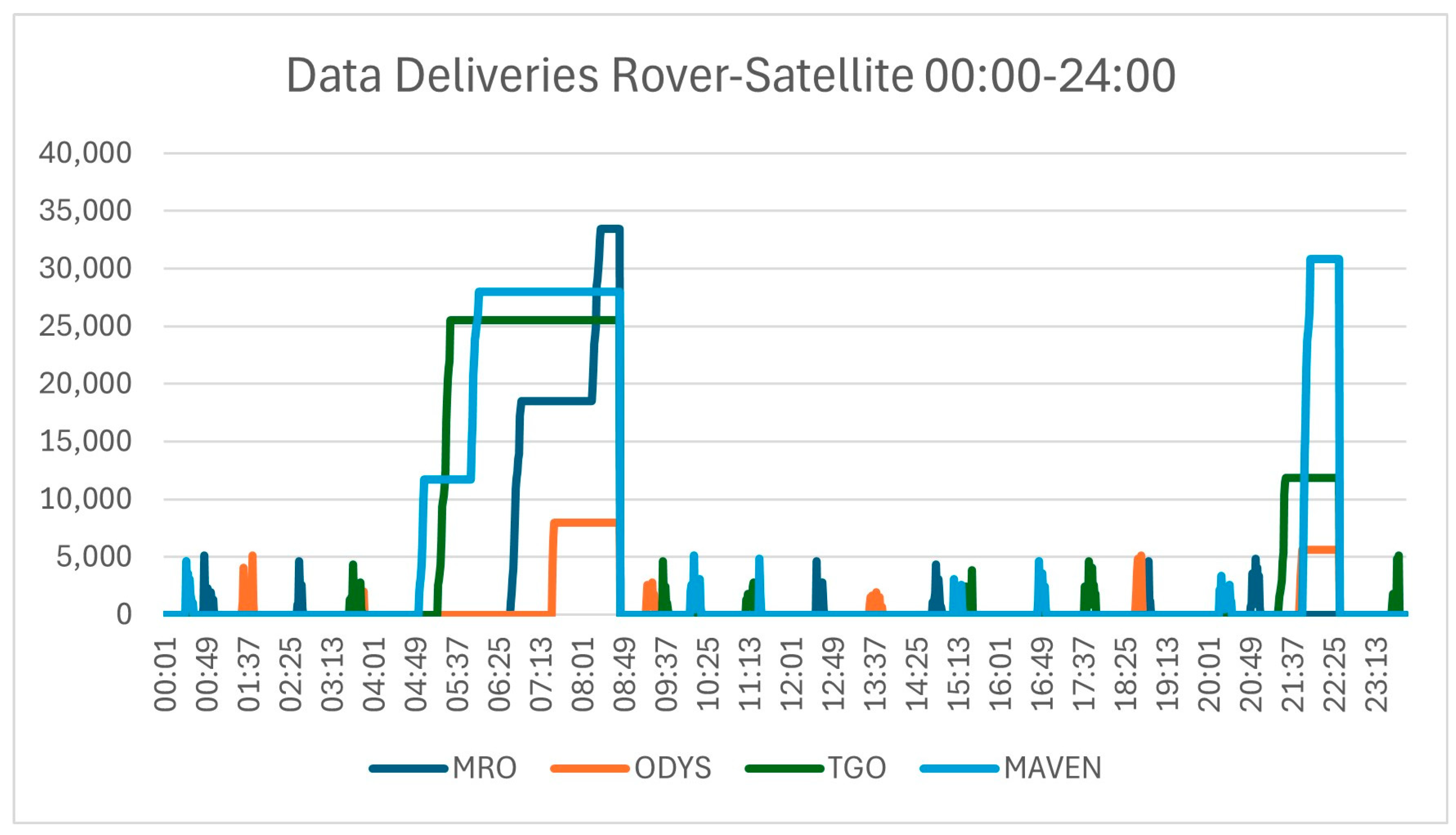
| Satellite & Storage | Rover | Mars Sol Time (MST) | Duration (Minutes) |
|---|---|---|---|
| MRO (20 GB) | PR | ∼2 AM, ∼8 AM, ∼2 PM, ∼8 PM | 8 to 12 |
| CR | ∼12 AM, ∼6 AM, ∼12 PM, ∼6 PM | ||
| Odyssey (8 MB) | PR | ∼3 AM, ∼9 AM, ∼3 PM, ∼9 PM | 9 to 15 |
| CR | ∼1 AM, ∼7 AM, ∼1 PM, ∼7 PM | ||
| TGO (16 GB) | PR | ∼5 AM, ∼11 AM, ∼5 PM, ∼11 PM | 9 to 15 |
| CR | ∼3 AM, ∼9 AM, ∼3 PM, ∼9 PM | ||
| MAVEN (16 GB) | Every 4.5 h | 3 to 10 | |
| Rover | Satellite | Contact Windows |
|---|---|---|
| PR | MRO | 02:34–02:40, 08:13–08:23, 14:44–14:54, 20:50–21:00 |
| Odyssey | 03:41–03:50, 09:15–09:25, 15:10–15:22, 21:46–21:58 | |
| TGO | 05:16–05:30, 11:10–11:24, 17:39–17:51, 23:32–23:41, | |
| MAVEN | 00:25–00:34, 05:54–06:03, 11:18–11:28, 16:45–16:55, 21:50–21:58 | |
| CR | MRO | 00:46–00:58, 06:39–06:51, 12:31–12:38, 18:48–18:54 |
| Odyssey | 01:30–01:43, 07:27–07:35, 13:32–13:46, 18:37–18:45 | |
| TGO | 03:34–03:48, 09:34–09:40, 15:19–15:30, 21:22–21:30 | |
| MAVEN | 04:54–05:00, 10:06–10:17, 15:09–15:24, 20:14–20:28, 01:29–01:41:00 |
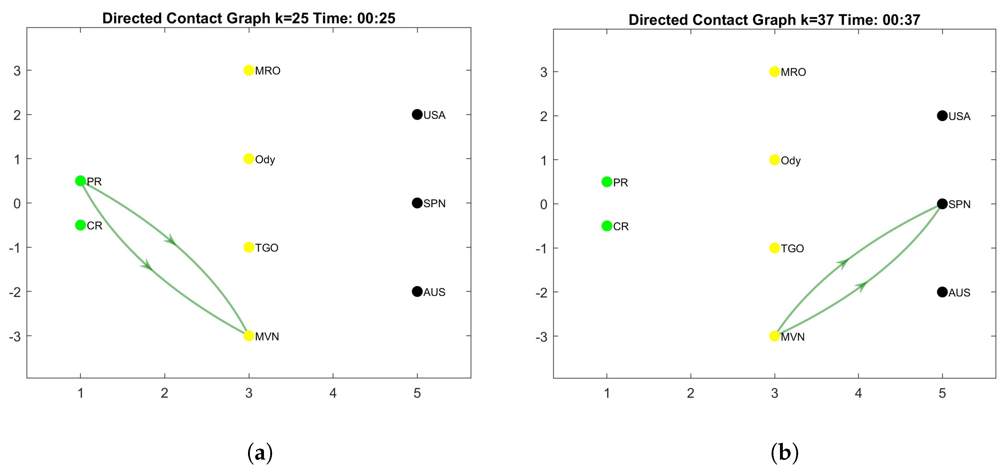
| Dep/Arr | Time | Packet Number | Routes | Data Size | Info |
|---|---|---|---|---|---|
| Dep | 00:25 | 2 | PR-MVN | 384 | Figure 4a |
| Dep | 00:26 | 18 | PR-MVN | 4600 | |
| Dep | 00:27 | 5 | PR-MVN | 1216 | |
| Dep | 00:28 | 14 | PR-MVN | 3584 | |
| Dep | 00:29 | 5 | PR-MVN | 1088 | |
| Arr | 00:37 | 2 | MVN-SPN | 384 | Figure 4b |
| Arr | 00:38 | 18 | MVN-SPN | 4600 | |
| Arr | 00:39 | 6 | MVN-SPN | 1216 | |
| Arr | 00:40 | 14 | MVN-SPN | 3584 | |
| Arr | 00:41 | 5 | MVN-SPN | 1088 |
| Dep/Arr | Time | Packet Number | Routes | Data Size | Info |
|---|---|---|---|---|---|
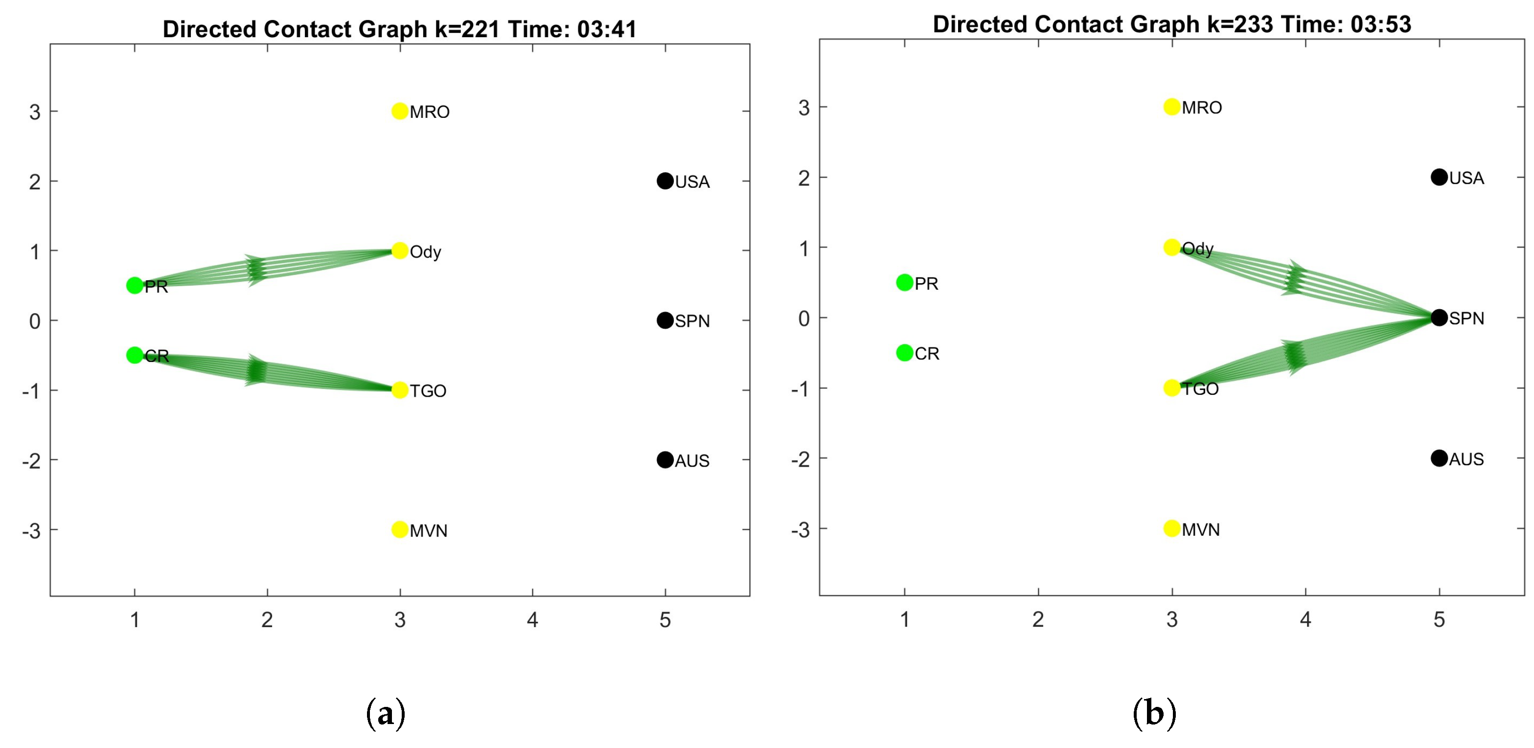
| Dep | 03:41 | 5 | PR-ODY | 1280 | Figure 5a |
| Dep | 8 | CR-TGO | 2048 | ||
| Dep | 03:42 | 4 | PR-ODY | 1024 | |
| Dep | 6 | CR-TGO | 1536 | ||
| Dep | 03:43 | 2 | PR-ODY | 512 | |
| Dep | 3 | CR-TGO | 768 | ||
| Dep | 03:44 | 4 | PR-ODY | 768 | |
| Dep | 5 | CR-TGO | 1280 | ||
| Arr | 03:53 | 5 | ODY-SPN | 1280 | |
| Arr | 8 | TGO-SPN | 2048 | Figure 5b | |
| Arr | 03:54 | 4 | ODY-SPN | 1024 | |
| Arr | 6 | TGO-SPN | 1536 | ||
| Arr | 03:55 | 2 | ODY-SPN | 512 | |
| Arr | 3 | CR-TGO | 768 | ||
| Arr | 03:56 | 4 | ODY-SPN | 768 | |
| Arr | 5 | TGO-SPN | 1280 |
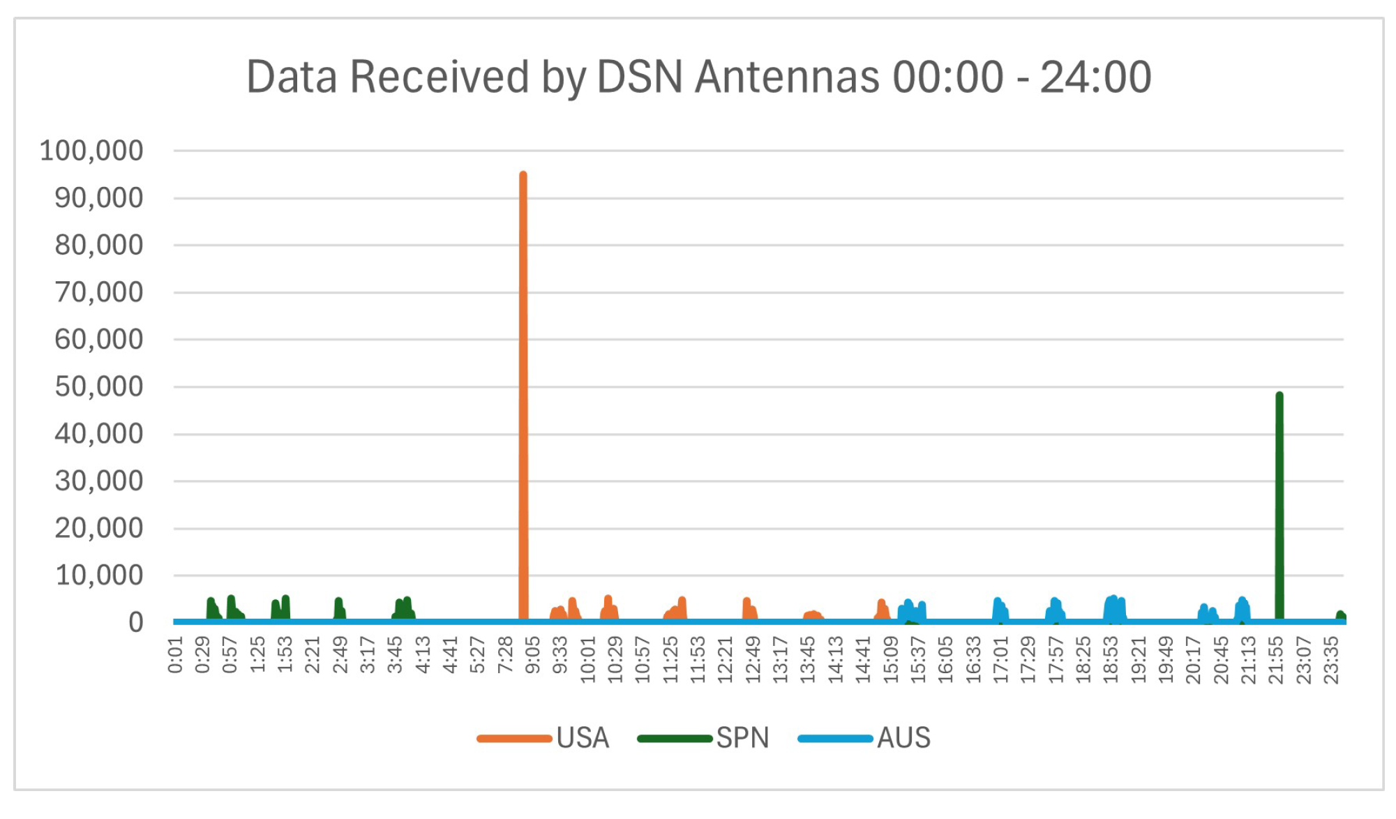
| Dep/Arr | Time | Routes | Total Data | Info |
|---|---|---|---|---|
| 04:50–04:53 | - | - | No contact | |
| Dep | 04:54–05:00 | CR-MVN | 11,712 | |
| 05:01–05:15 | - | - | No contact | |
| Dep | 05:16–05:30 | PR-TGO | 25,536 | |
| 05:31–05:53 | - | - | No contact | |
| Dep | 05:54–06:03 | PR-MVN | 16,256 | |
| 06:04–06:38 | - | - | No contact | |
| Dep | 06:39–06:51 | CR-MRO | 18,496 | |
| 06:52–07:26 | - | - | No contact | |
| Dep | 07:27–07:35 | CR-ODY | 8000 | |
| 07:36–08:12 | - | - | No contact | |
| Dep | 08:13–08:23 | PR-MRO | 14,976 | |
| 08:24–08:55 | - | - | No contact | |
| Arr | 08:56 | MVN-USA | 27,968 | |
| TGO-USA | 25,536 | |||
| MRO-USA | 33,472 | |||
| ODY-USA | 8000 | Loss 12,224 |
| Dep/Arr | Time | Routes | Total Data | Info |
|---|---|---|---|---|
| Dep | 21:22–21:31 | CR-TGO | 11,840 | |
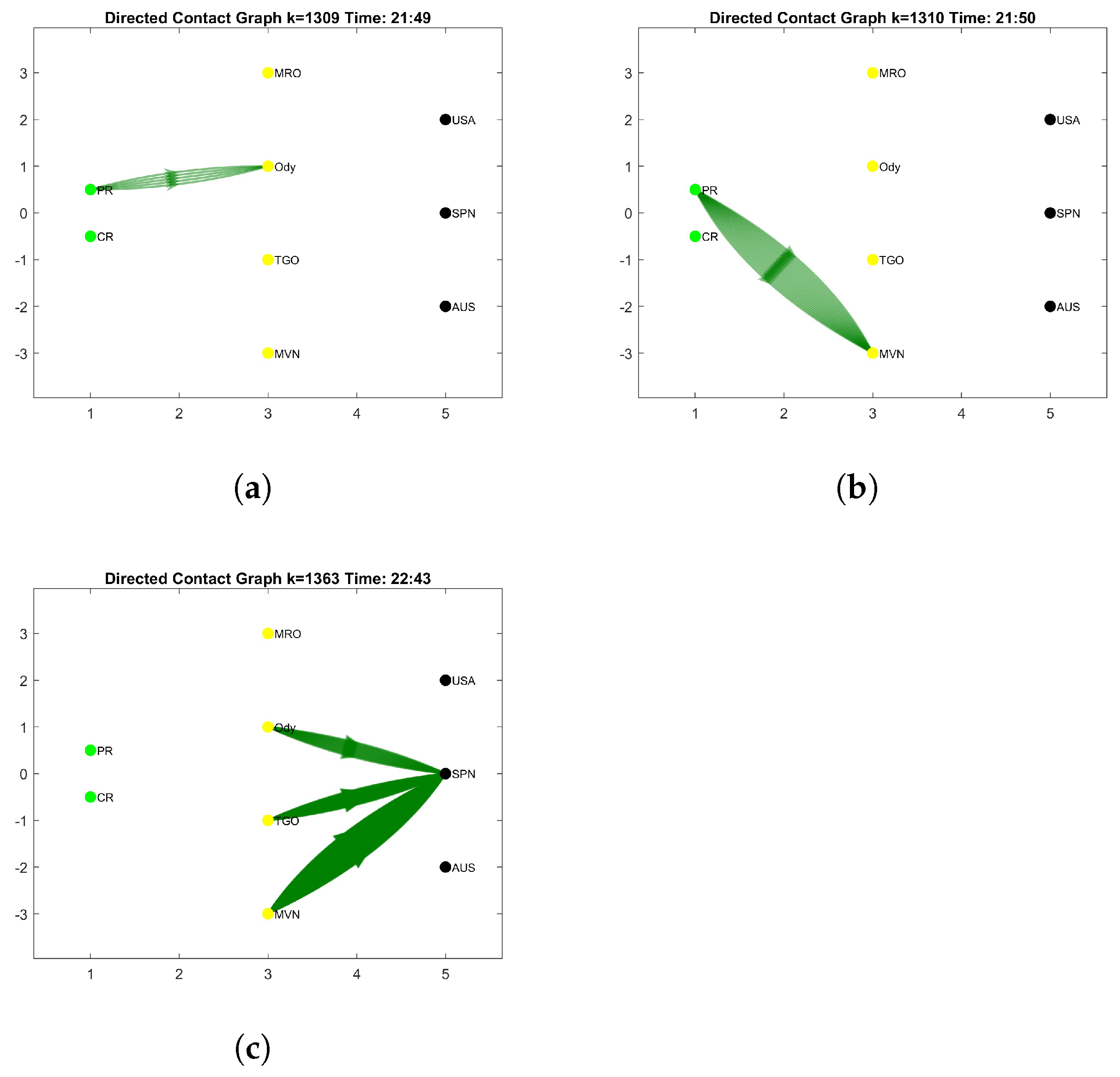
| Dep | 21:46–21:49 | PR-ODY | 5632 | |
| Dep | 21:50–21:58 | PR-MVN | 30,848 | |
| Dep | 21:59–22:31 | - | - | No contact |
| Arr | 22:43 | TGO-SPN | 1180 | Figure 6c |
| ODY-SPN | 5632 | |||
| MVN-SPN | 30,848 |
Disclaimer/Publisher’s Note: The statements, opinions and data contained in all publications are solely those of the individual author(s) and contributor(s) and not of MDPI and/or the editor(s). MDPI and/or the editor(s) disclaim responsibility for any injury to people or property resulting from any ideas, methods, instructions or products referred to in the content. |
© 2025 by the authors. Licensee MDPI, Basel, Switzerland. This article is an open access article distributed under the terms and conditions of the Creative Commons Attribution (CC BY) license (https://creativecommons.org/licenses/by/4.0/).
Share and Cite
Suhardiman, B.; Sidarto, K.A.; Sumarti, N. A Simulation of Contact Graph Routing for Mars–Earth Data Communication. Algorithms 2025, 18, 293. https://doi.org/10.3390/a18050293
Suhardiman B, Sidarto KA, Sumarti N. A Simulation of Contact Graph Routing for Mars–Earth Data Communication. Algorithms. 2025; 18(5):293. https://doi.org/10.3390/a18050293
Chicago/Turabian StyleSuhardiman, Basuki, Kuntjoro Adji Sidarto, and Novriana Sumarti. 2025. "A Simulation of Contact Graph Routing for Mars–Earth Data Communication" Algorithms 18, no. 5: 293. https://doi.org/10.3390/a18050293
APA StyleSuhardiman, B., Sidarto, K. A., & Sumarti, N. (2025). A Simulation of Contact Graph Routing for Mars–Earth Data Communication. Algorithms, 18(5), 293. https://doi.org/10.3390/a18050293