Generation of Realistic Synthetic Load Profile Based on the Markov Chains Theory: Methodology and Case Studies
Abstract
1. Introduction
2. Materials and Methods
2.1. Basic Requirements
- The random generator should allow generating data with a time step of 15 min or less.
- The generated synthetic data should have an identical statistical distribution to the training data.
- The generated synthetic data should have identical probabilistic properties as the training data.
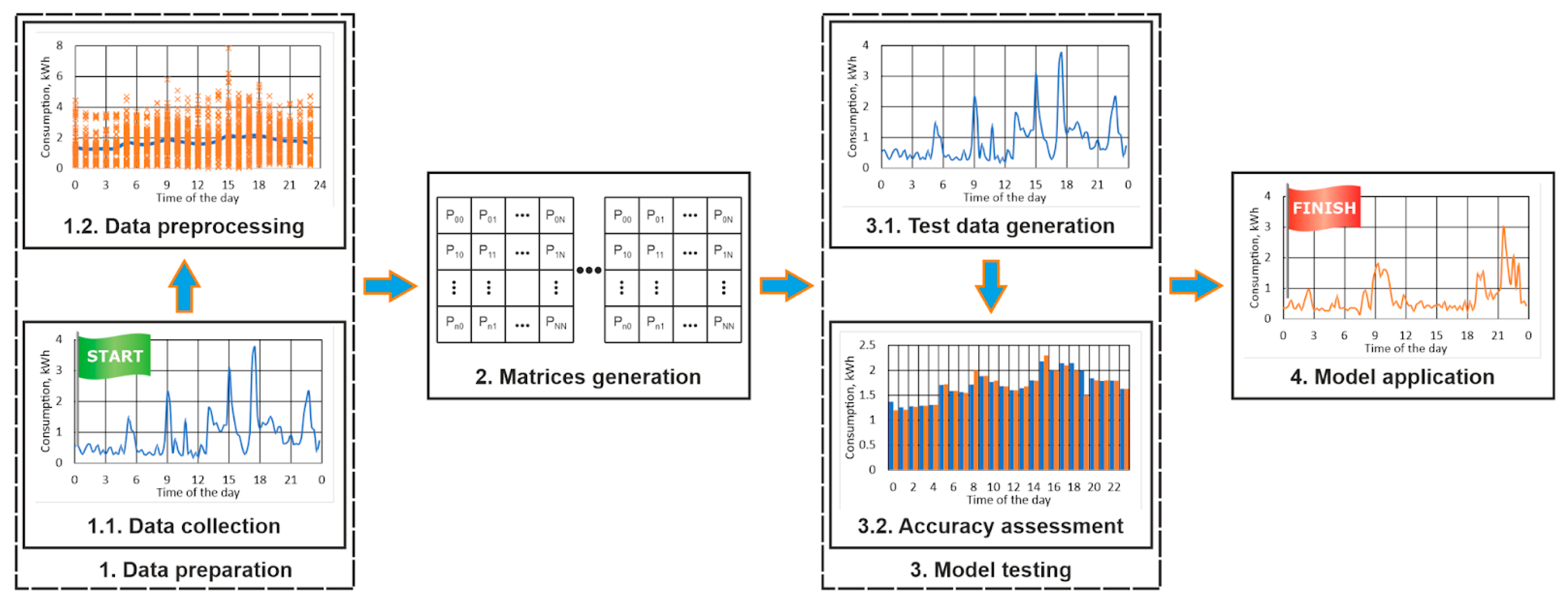
2.2. Methodology
- a timestamp, including the date and time of the measurement;
- instantaneous (or average) power of the load for the corresponding moment.
- The time series is verified for inconsistencies, which should either be excluded or corrected (if applicable). Such situations might include records with empty values, negative values, unrealistically high values, etc. This verification could be made either manually or using different tools and approaches, including statistical methods for outlier detection.
- If the time step of the series is lower than intended, it should be increased by choosing an appropriate approach. For example, if the time of discretization of the dataset is 5 min, and it should be analyzed in 15 min batches, then the data should be resampled. The new 15 min records could be formed either by selecting the corresponding records or by averaging them with the nearby records.
- The time series should be divided into appropriate batches, depending on its seasonality. For example, if the load profile characteristics are different for the different months of the year, then it should be analyzed independently for each month. In the current study, we have adopted this approach.
- -
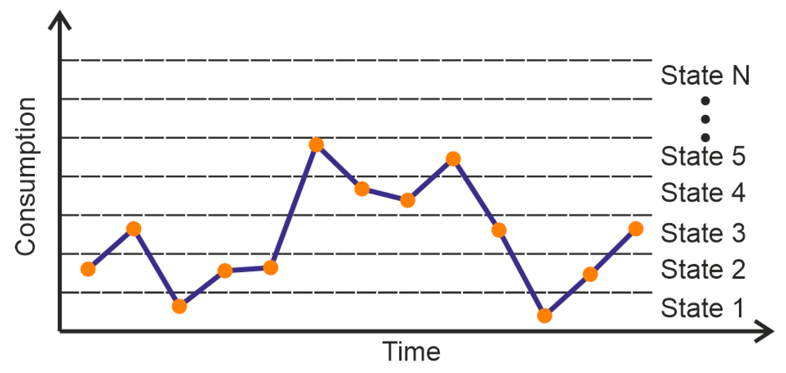
- Choosing the number of states, i.e., the dimensionality of the matrices. The data are divided into N states (Figure 3) of equal width, which is estimated according to
- -
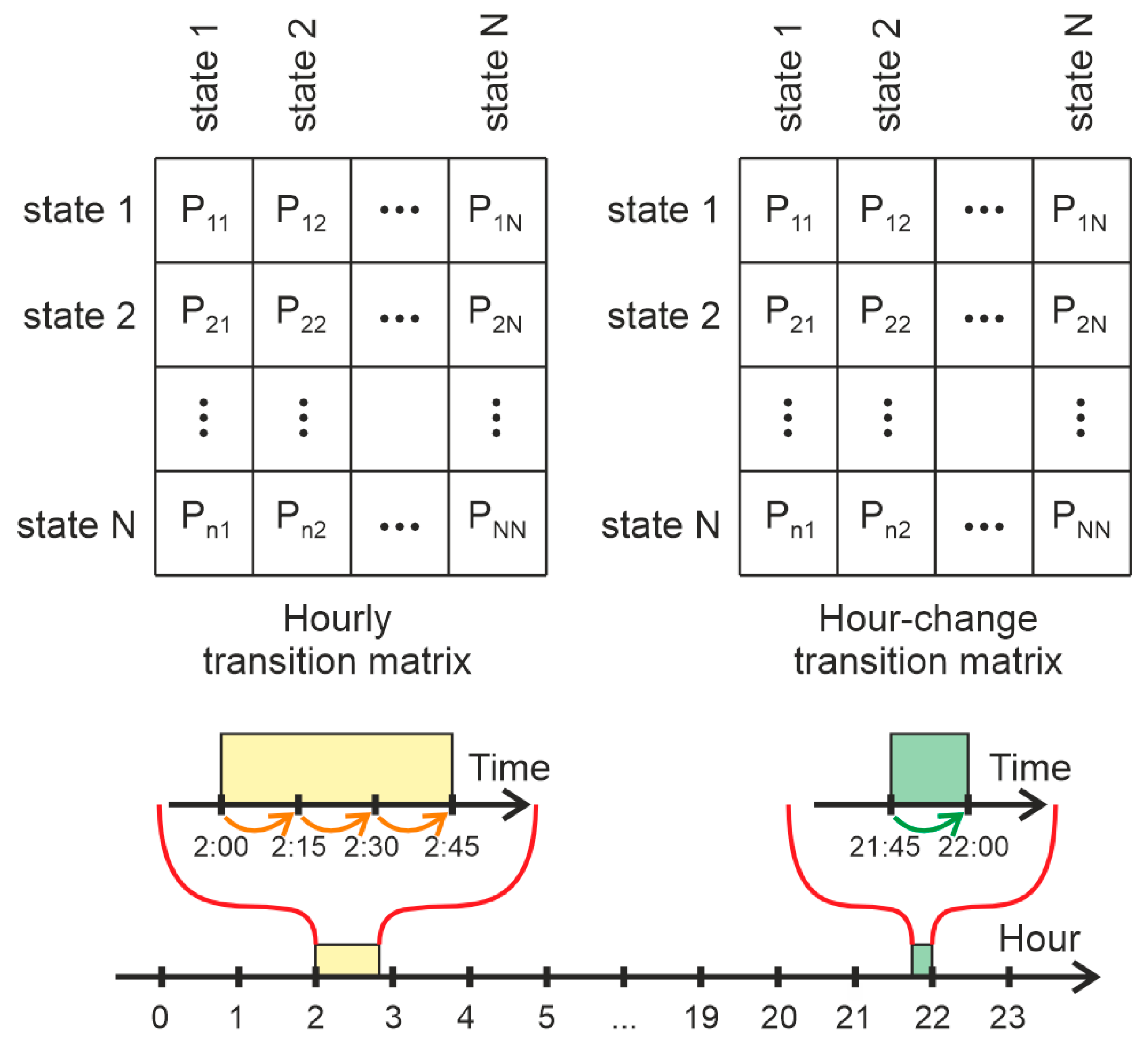
- Generating 24 transition matrices for each hour of the day, based on the Markov chain theory. In other words, each discrete sample of the load profile data is classified into one of the N states and the probabilities of jumping from each state to all other states are estimated for each hour of the day (Figure 4). These matrices are generated using all pairs of sequential records, which belong to the same hour of the day (for example, if the time of discretization is 15 min, the records at 09:30 and 09:45 are consecutive and belong to the same hour).
- -
- Generating 24 transition matrices containing the probabilities for changing states when an hour is changed (Figure 4). They are based on all pairs of sequential records, which belong to different hours (for example, if the time of discretization is 15 min, the records at 9:45 and 10:00 belong to different hours of the day).
- The initial hour and state for the data (for example, 0 h) are chosen—the chosen state must have non-zero probability in the corresponding hourly transition matrix;
- The next state of the synthetic data is generated randomly, according to the probability distribution for the current state in the transmission matrix, which could be achieved as shown in Algorithm 1.
| Algorithm 1. Generating the next state according to the transition matrix probabilities. |
| Let Xt be the last state NumberOfTransitions = Count(Mh:h, Xt)//Get the total number of possible transitions (according to the original dataset) from the current state Xt RandomNumber = rand(1 … NumberOfTransitions)//get a random number between 1 and NumberOfTransitions NextState = 0//initialize while RandomNumber > 0 { if RandomNumber <= Mh:h(Xt, NextState)//Mh:h(Xt, NextState) are the number of possible transitions from Xt to NextState { Xt+1 = NextState;//the next state has been randomly generated break; } RandomNumber = RandomNumber − Mh:h(Xt, NextState); NextState = NextState + 1 } |
- Once the new state St+1 is generated, the value of the next sample is estimated according towhere random(0 …StateWidth) returns a random value between 0 and StateWidth. When the current and the next generated records belong to the same hour of the day, the corresponding hourly transition matrix is used; if they belong to different hours, the corresponding hour-change transition matrix is used.
| Algorithm 2. Handling of the situation where the current state exists in the hour-change matrix with a zero probability. |
| Let Xt be the last state for the hour h if the probability for the current state in the transition matrix Mh:h+1 (the matrix, describing the transition between the h hour and the h + 1 hour) is 0: { repeat N times: { Xt = Mh:h(Xt−1)//Generate the last state Xt again (the transition between Xt−1 and Xt) if the transition probability from state Xt in Mh:h+1 is nonzero: { //Continue with the newly obtained state Xt; break; } } } if an appropriate state Xt was obtained, for which a transition exists in the matrix Mh:h+1: { Xt+1 = Mh:h+1(Xt)//generate the next state Xt+1 from the current state Xt } else { Xt+1 = rand(all states)//randomly choose a new state from all states in Mh:h+1. } |
- The standard deviation of the energy consumption:
- The variance of the energy consumption:
- the Frobenius distance:
- the coefficient of determination (R2) [35]—in order to apply it on matrices, they should first be converted from n × n dimensional ones to an n2 dimensional vector.
2.3. Means of the Investigation
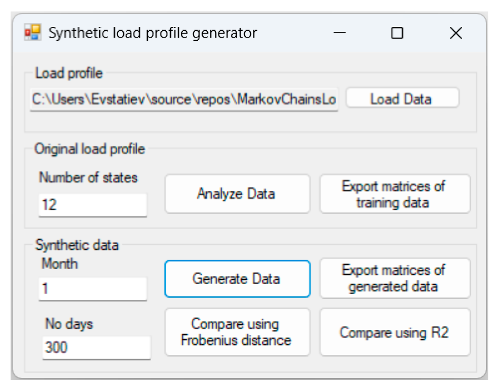
- The “Load Data” button loads the training dataset from a tab-delimited file containing the month of the year, the hour of the day, and the power consumption (Table 1). The developed tool assumes that the data has a 15 min time step.
- 2.
- The “Analyze Data” button estimates 24 hourly and 24 h-change transition matrices, based on the provided dataset and the defined number of states (in the “Number of states” field).
- 3.
- The “Generate Data” button generates synthetic data for the defined number of days (in the “No days” field) and month (in the “Month” field) with a 15 min time step. The synthetic data are automatically exported in a tab-delimited file.
- 4.
- The buttons “Export matrices of training data” and “Export matrices of generated data” export the hourly and hour-change transition matrices of the training and synthetic datasets, respectively.
- 5.
- The button “Compare using Frobenius distance” estimates the Frobenius distances between each two corresponding matrices of the original and generated datasets and exports them in a tab-delimited file.
- 6.
- The button “Compare using R2” estimates the R2 values between each two corresponding matrices of the original and generated datasets and exports them in a tab-delimited file.
3. Results and Discussion
3.1. Testing Datasets
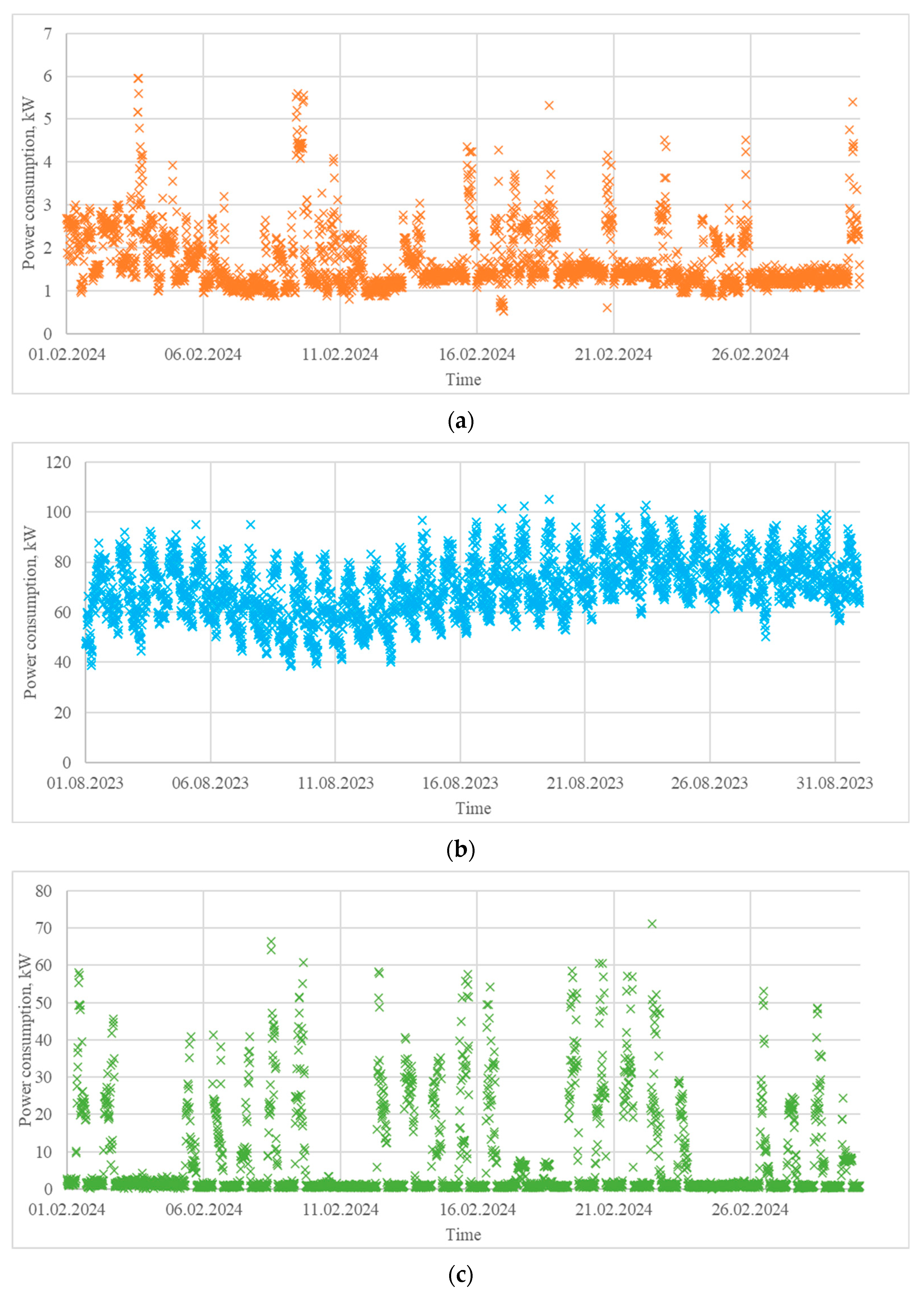
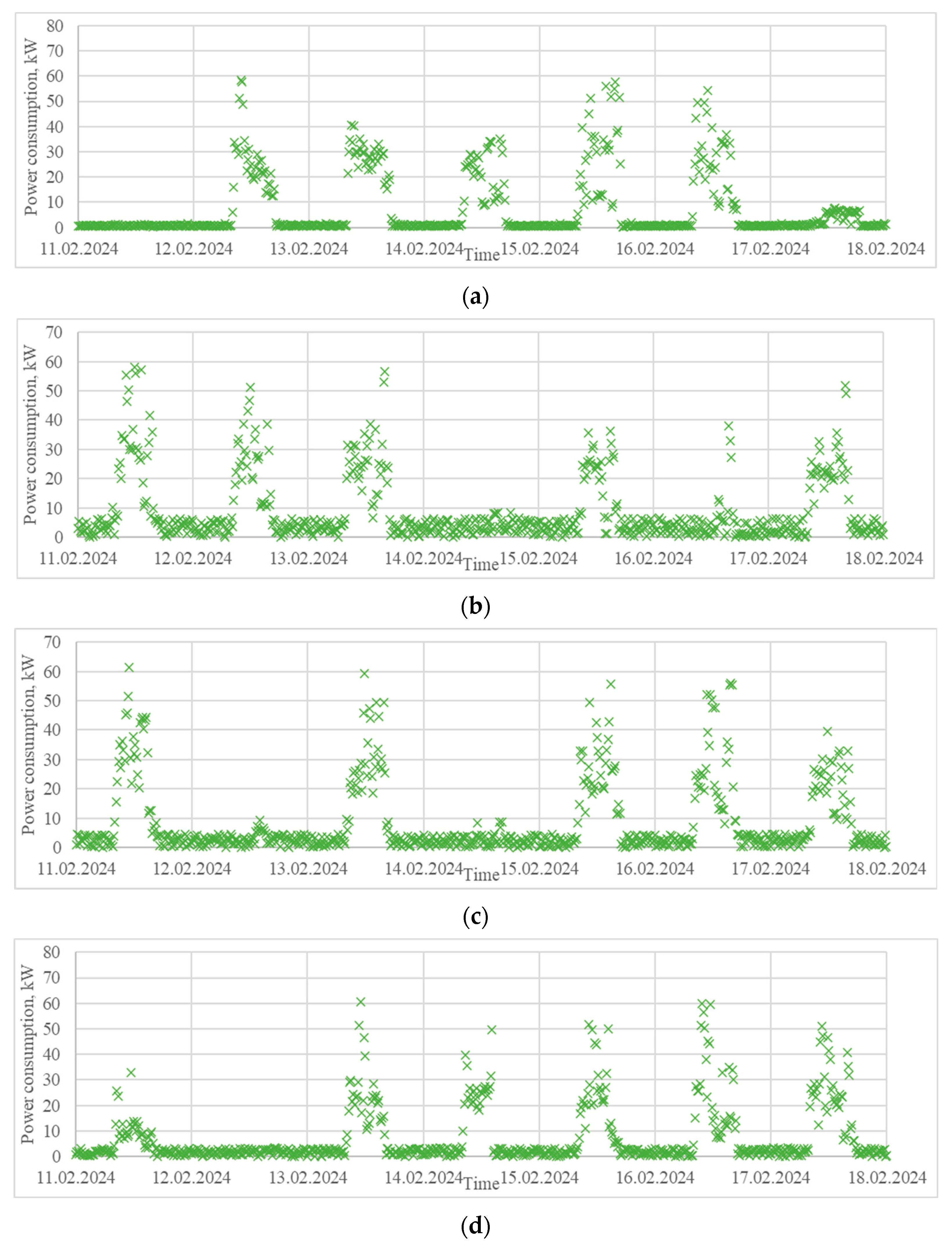
- A load profile extracted from a house located in the region of Ruse, Bulgaria, in the period 1–29 February 2024 (Figure 6a). It is characterized by power consumption varying in a wide range and significant peaks during the weekends. Residential load profiles are generally influenced by many factors, such as the type of day (weekday or weekend), hour of the day, meteorological conditions, people’s lifestyle, holidays, etc.
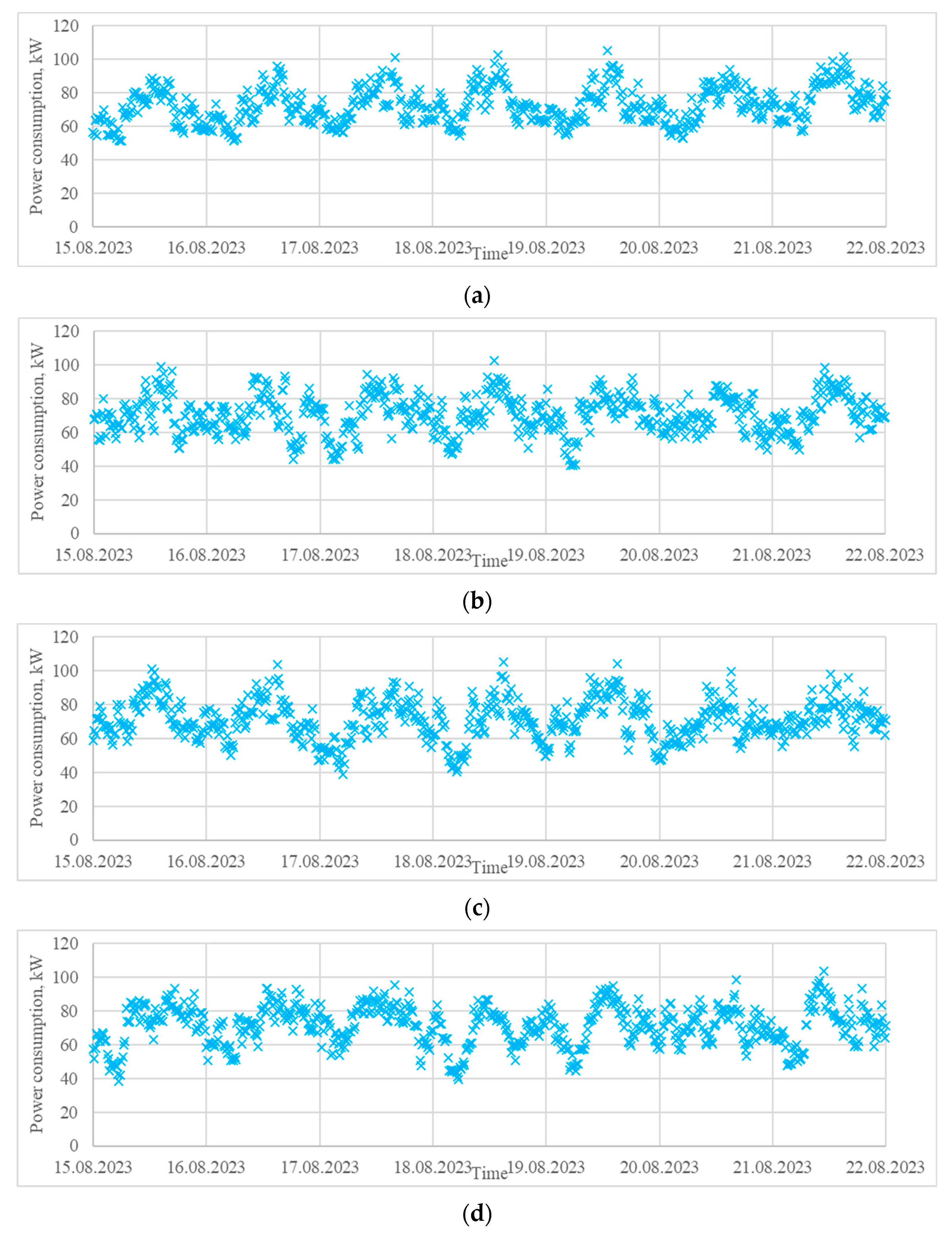
- A load profile of a pig farm located in the region of Silistra, Bulgaria, in the period 1–31 August 2023 (Figure 6b). It is characterized by relatively similar daily variations, which can be explained by the agrotechnological requirements. Load profiles in livestock farming are influenced mostly by the schedule of the technological processes (lighting, feeding, ventilation, etc.) and the meteorological conditions.
- A load profile of a printing house, located in the region of Varna, Bulgaria, for the period 1–29 February 2024 (Figure 6c). It is characterized by significant electrical consumption during the working hours of the weekdays and almost zero consumption during the rest of the time. Industrial load profiles are greatly influenced by factors such as the type of day (weekday or weekend), hour of the day, daily schedule, holidays, and the meteorological conditions.
3.2. Comparison Between the Training and Synthetic Data
3.2.1. Case Study 1: Generation of Synthetic Power Consumption Data for a Domestic Consumer
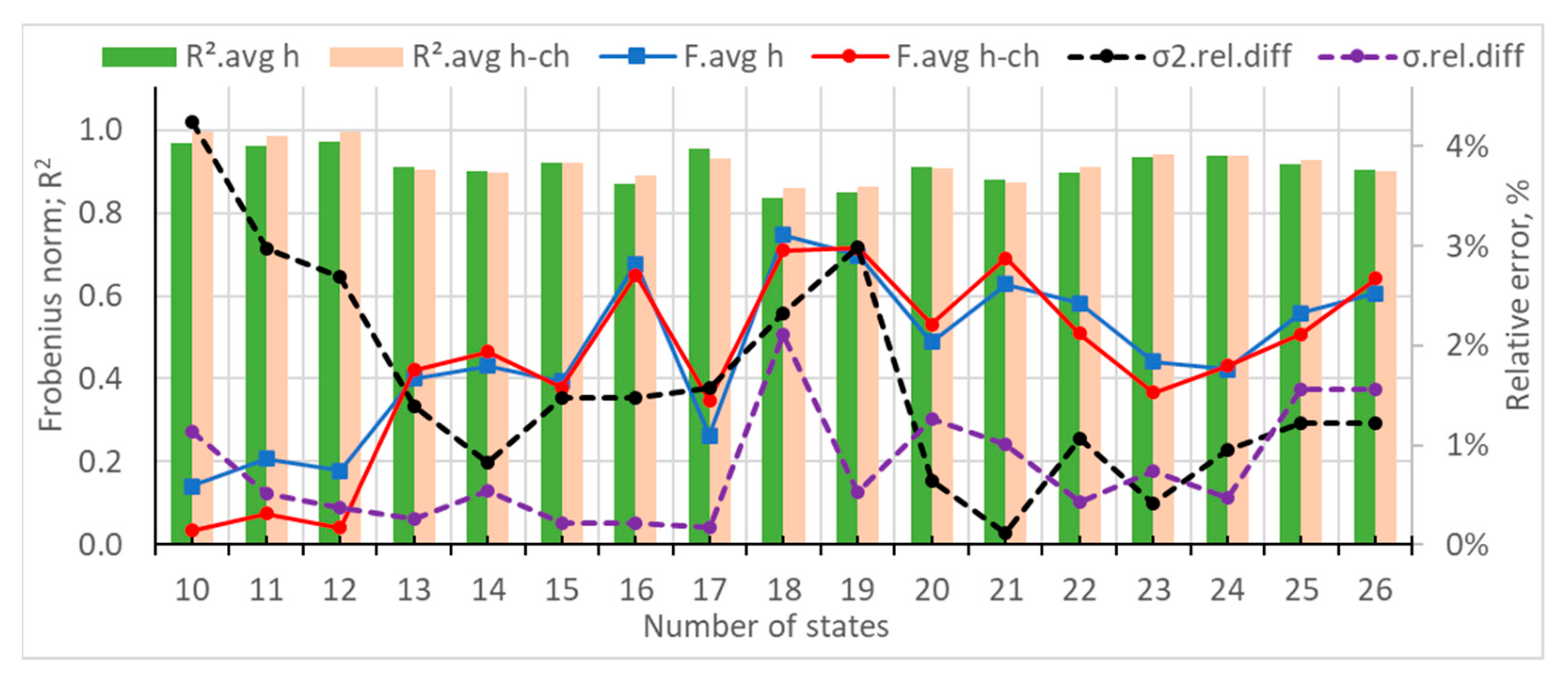
- Matrices were generated according to Step 2 of the methodology.
- 10,000 days of synthetic data were generated according to Step 3.1 from the methodology to make sure the long-term trend of the generated data has reached the final probability distribution vector.
- The matrices of the synthetic and of the original data were compared using the Frobenius distance and R2, according to Step 3.2 of the methodology.
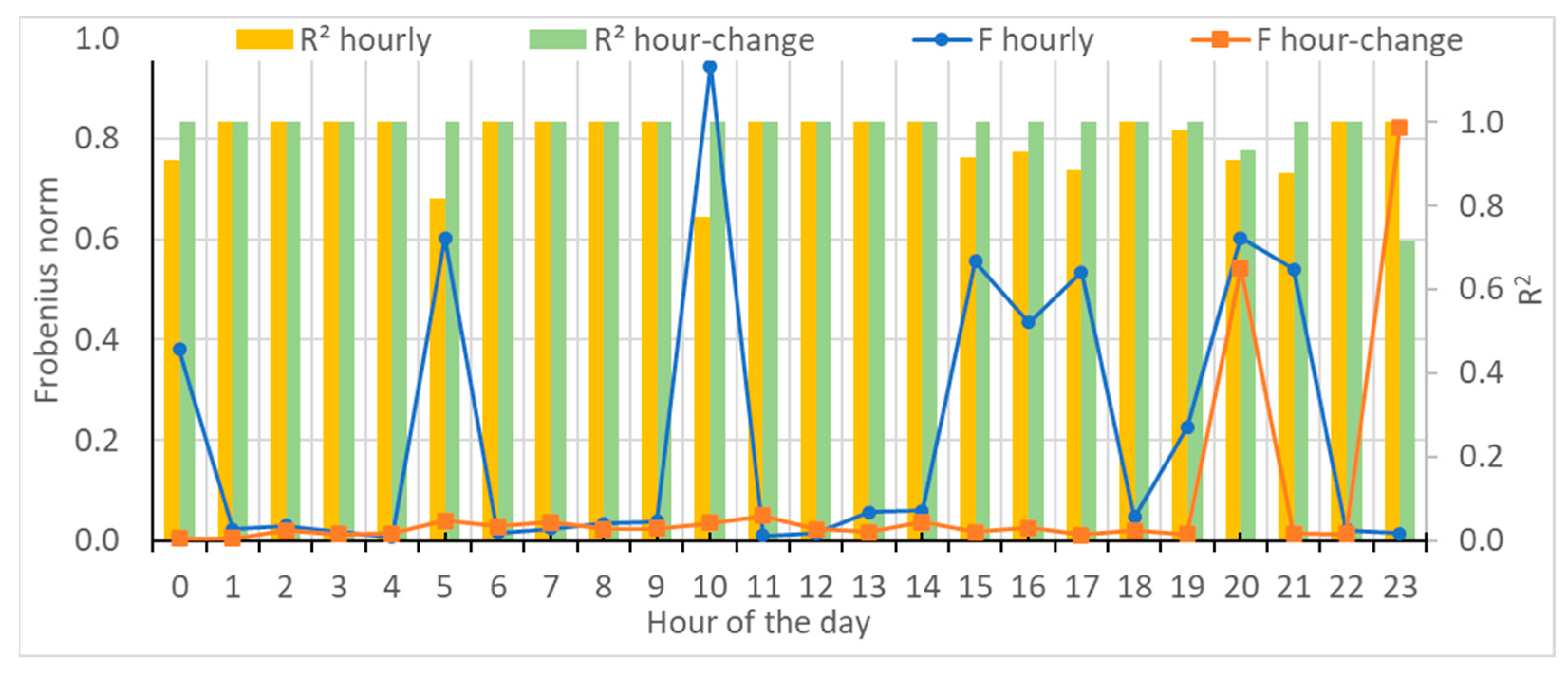
- The average Frobenius distance and R2 were estimated for each hour of the day.
- The relative difference between the variance and standard deviation of the original and the synthetic data was obtained.
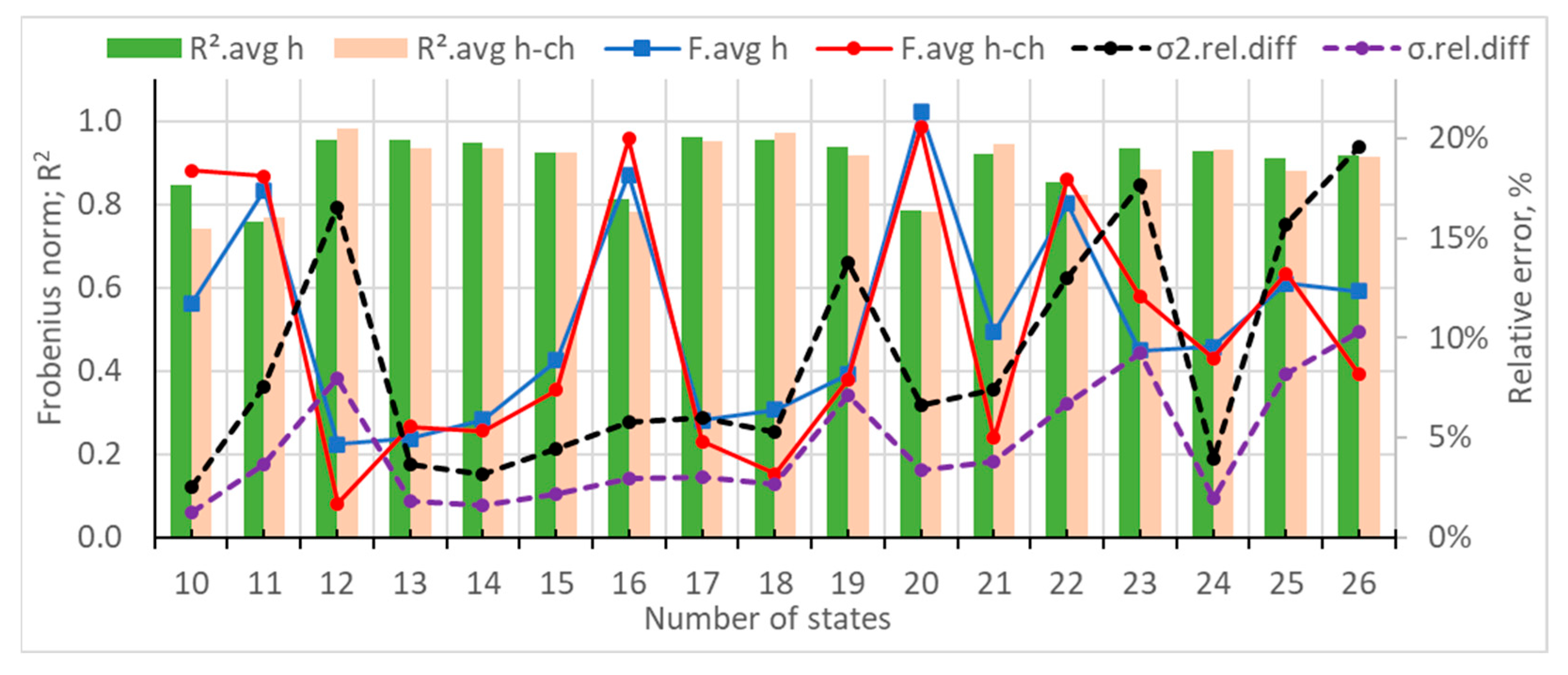
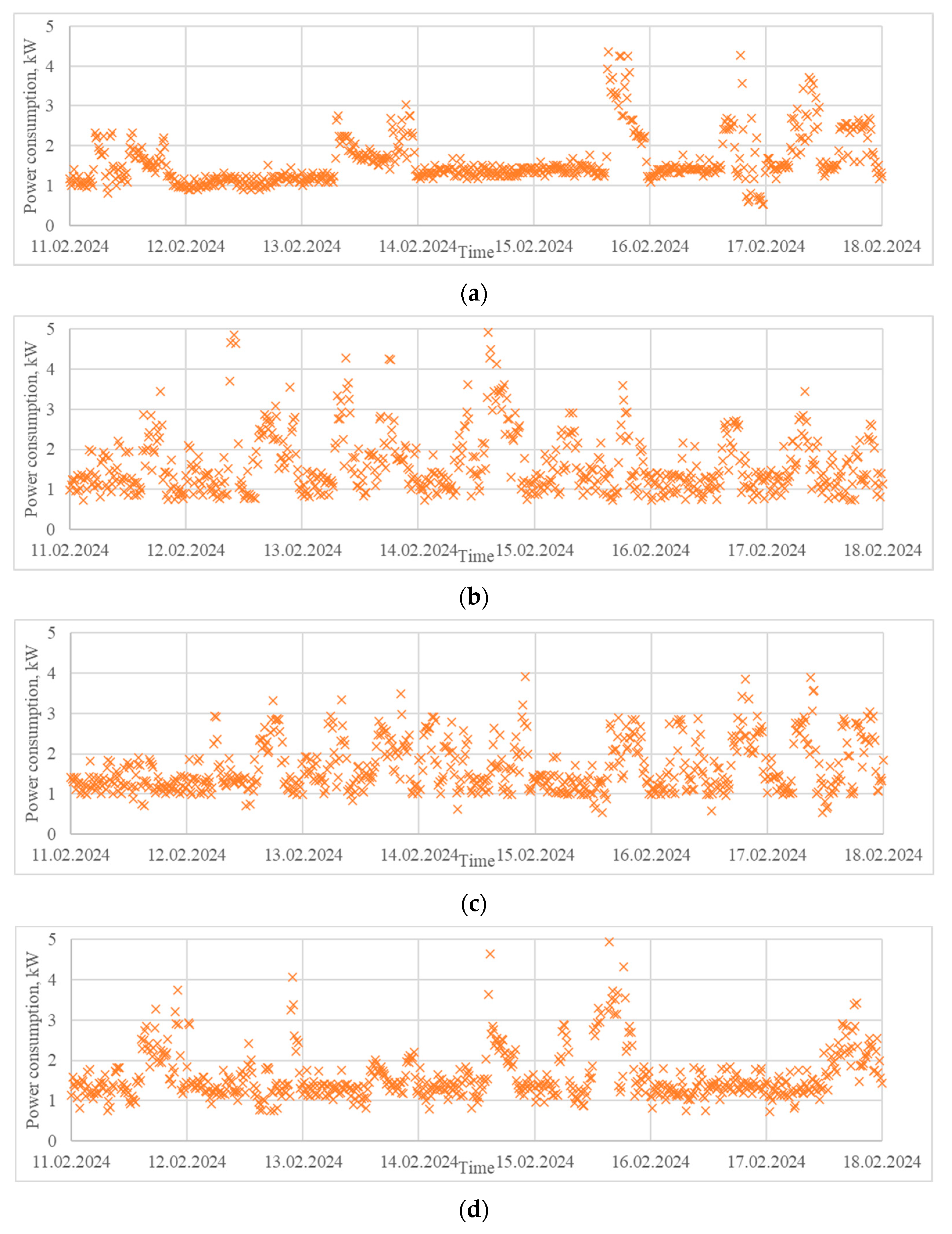
- The generated data with 12 states, which was characterized by the lowest Frobenius distances and the highest R2 values, but with higher relative error for the variance and standard deviation.
- The generated data with 18 states, which was characterized by a local minimum of the Frobenius distances, high R2 values, and local minimums of the statistical measures.
- The generated data with 24 states, which was characterized by local minimums of the Frobenius distances and the statistical measures, as well as high R2 values.
3.2.2. Case Study 2: Generation of Synthetic Power Consumption Data for a Pig Farm
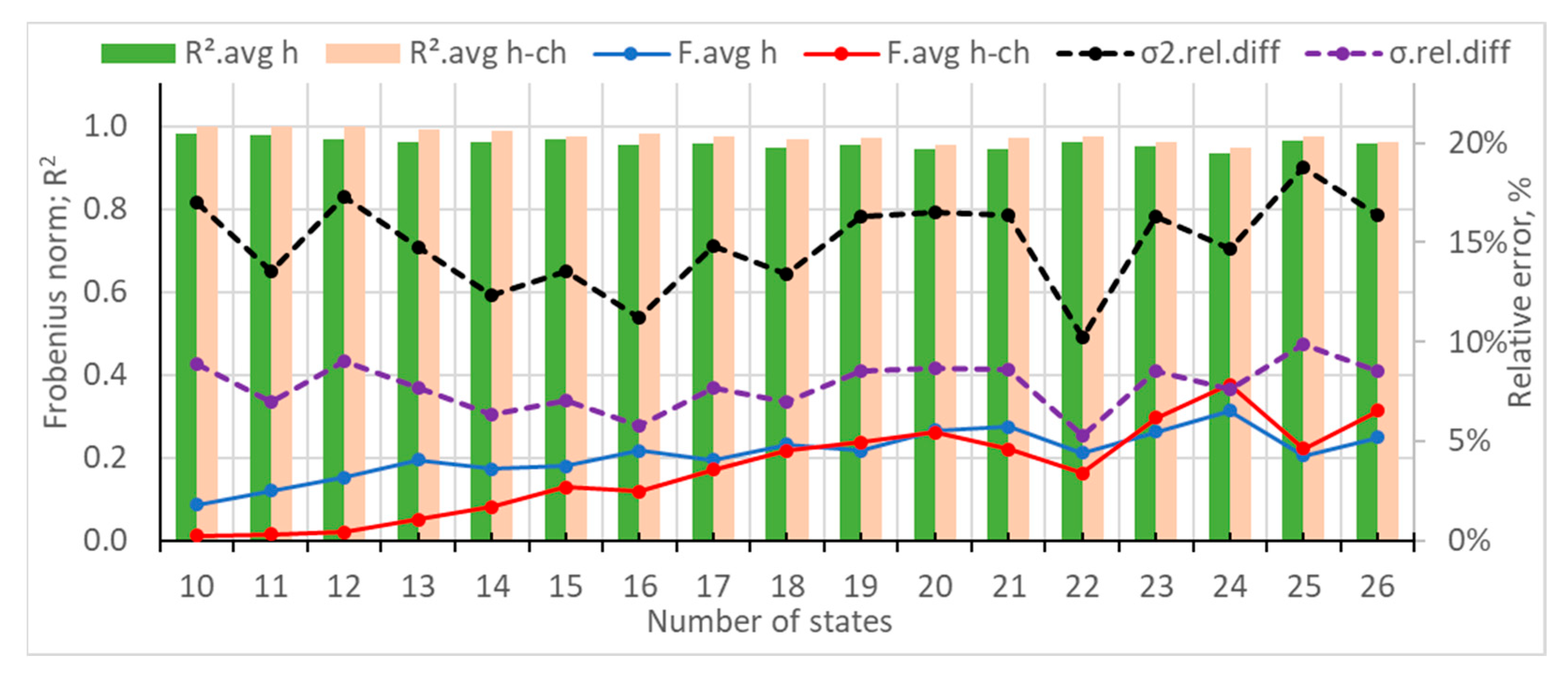
- the generated data with 12 states, for which all measures except for the variance have near-optimal values;
- the generated data for 17 states, for which all measures except the variance have a local peak value;
- the generated data for 23 states, for which there are local peak values for the Frobenius distances, R2, and the variance.
3.2.3. Case Study 3: Generation of Synthetic Power Consumption Data for a Printing House
- the generated data with 11 states, for which all indicators have peaks or close-to-optimal values;
- the generated data with 16 states, for which the statistical measures have local minimums and the probabilistic measures are close to optimal;
- the generated data with 22 states, for which the Frobenius distances and the R2 coefficients have local peaks, and the statistical measures have minimums.
3.3. Discussion and General Recommendations for the Application of the Proposed Methodology
- The Frobenius distances, describing the difference between the transition matrices of the original dataset and of the generated data, are as close as possible to 0.
- The R2 coefficients, describing how well the generated transition matrices describe the original ones, are as close as possible to 1.
- The statistical measures of the generated data, such as its variance and standard deviation, are as close as possible to the statistical measures of the original dataset.
- The Frobenius distances and R2 coefficients were usually closer to their optimal values for a lower number of states.
- The difference between the statistical measures of the generated and original datasets could vary in a wide range, depending on the number of states of the transition matrices.
- The generated datasets with a lower number of states were usually more scattered than the training ones.
- Local minimums of the average Frobenius distances and/or local maximums of the average R2 coefficients should be looked for at a higher number of states of the transition matrices. It is recommended that the number of states be more than 20 or at least 15.
- Local minimums of the statistical measures of variance and/or standard deviation could be looked for.
- The optimal number of states can be chosen for the situation where the measures from p. 1 and p. 2 have their local peak values or values that are very close to them.
4. Conclusions
- When possible, the number of states of the transition matrices should be 15 or more to reduce the scattering of the synthetic data.
- The number of states can be chosen by looking for local peaks of the Frobenius distance, R2 coefficients, relative differences of the variance, and/or standard deviation, which do not differ significantly from their optimal values.
Author Contributions
Funding
Data Availability Statement
Conflicts of Interest
Abbreviations
| ANN | artificial neural network |
| GAN | generative adversarial networks |
| KNN | k-nearest neighbor |
| LLMs | large language models |
| ML | machine learning |
| VAEs | variational autoencoders |
| wRNG | weighted random number generator |
| σ | standard deviation |
| σ.rel.diff | relative error of the standard deviation |
| σ2 | variance |
| σ2.rel.diff | relative error of the variance |
| F | Frobenius distance |
| F.avg h | average Frobenius distance of the hourly matrices |
| F.avg h-ch | average Frobenius distance of the hour-change matrices |
| N | number of states |
| Pmax | maximal power consumption |
| Pmin | minimal power consumption |
| R2 | coefficient of determination |
| R2.avg h | average R2 of the hourly matrices |
| R2.avg h-ch | average R2 of the hour-change matrices |
References
- Endres, M.; Mannarapotta, V.A.; Tran, T.S. Synthetic data generation: A comparative study. In Proceedings of the 26th International Database Engineered Applications Symposium, Budapest, Hungary, 22–24 August 2022; pp. 94–102. [Google Scholar]
- Sandhaas, A.; Kim, H.; Hartmann, N. Methodology for Generating Synthetic Load Profiles for Different Industry Types. Energies 2022, 15, 3683. [Google Scholar] [CrossRef]
- Jordon, J.; Szpruch, L.; Houssiau, F.; Bottarelli, M.; Cherubin, G.; Maple, C.; Cohen, S.; Weller, A. Synthetic Data—What, Why and How? Royal Society: London, UK, 2022; Available online: https://royalsociety.org/-/media/policy/projects/privacy-enhancing-technologies/Synthetic_Data_Survey-24.pdf (accessed on 15 March 2025).
- Hong, T.; Pinson, P.; Wang, Y.; Weron, R.; Yang, D.; Zareipour, H. Energy forecasting: A review and outlook. IEEE Open Access J. Power Energy 2020, 7, 376–388. [Google Scholar] [CrossRef]
- Proedrou, E. A comprehensive review of residential electricity load profile models. IEEE Access 2021, 9, 12114–12133. [Google Scholar] [CrossRef]
- Viana, D.; Teixeira, R.; Baptista, J.; Pinto, T. Synthetic Data Generation Models for Time Series: A Literature Review. In Proceedings of the 2024 International Conference on Electrical, Computer and Energy Technologies (ICECET), Sydney, Australia, 25–27 July 2024; pp. 1–6. [Google Scholar] [CrossRef]
- Bauer, A.; Trapp, S.; Stenger, M.; Leppich, R.; Kounev, S.; Leznik, M.; Foster, I. Comprehensive exploration of synthetic data generation: A survey. arXiv 2024, arXiv:2401.02524. [Google Scholar] [CrossRef]
- Lu, Y.; Shen, M.; Wang, H.; Wang, X.; van Rechem, C.; Fu, T.; Wei, W. Machine learning for synthetic data generation: A review. arXiv 2023, arXiv:2302.04062. [Google Scholar] [CrossRef]
- Jacobsen, B.N. Machine learning and the politics of synthetic data. Big Data Soc. 2023, 10, 20539517221145372. [Google Scholar] [CrossRef]
- Gandoman, F.H.; Aleem, S.H.A.; Omar, N.; Ahmadi, A.; Alenezi, F.Q. Short-term solar power forecasting considering cloud coverage and ambient temperature variation effects. Renew. Energy 2018, 123, 793–805. [Google Scholar] [CrossRef]
- Triastcyn, A.; Faltings, B. Generating Higher-Fidelity Synthetic Datasets with Privacy Guarantees. Algorithms 2022, 15, 232. [Google Scholar] [CrossRef]
- Zaini, F.A.; Sulaima, M.F.; Razak, I.A.W.A.; Othman, M.L.; Mokhlis, H. Improved Bacterial Foraging Optimization Algorithm with Machine Learning-Driven Short-Term Electricity Load Forecasting: A Case Study in Peninsular Malaysia. Algorithms 2024, 17, 510. [Google Scholar] [CrossRef]
- Lázaro, C.; Angulo, C. Iterative Application of UMAP-Based Algorithms for Fully Synthetic Healthcare Tabular Data Generation. Algorithms 2024, 17, 591. [Google Scholar] [CrossRef]
- Yue, Y.; Li, Y.; Yi, K.; Wu, Z. Synthetic data approach for classification and regression. In Proceedings of the 2018 IEEE 29th International Conference on Application-specific Systems, Architectures and Processors (ASAP), Milan, Italy, 10–12 July 2018; IEEE: New York, NY, USA, 2018; pp. 1–8. [Google Scholar] [CrossRef]
- Goyal, M.; Mahmoud, Q.H. A Systematic Review of Synthetic Data Generation Techniques Using Generative AI. Electronics 2024, 13, 3509. [Google Scholar] [CrossRef]
- Pan, Z.; Wang, J.; Liao, W.; Chen, H.; Yuan, D.; Zhu, W.; Fang, X.; Zhu, Z. Data-Driven EV Load Profiles Generation Using a Variational Auto-Encoder. Energies 2019, 12, 849. [Google Scholar] [CrossRef]
- Wang, C.; Tindemans, S.H.; Palensky, P. Generating contextual load profiles using a conditional variational autoencoder. In Proceedings of the 2022 IEEE PES Innovative Smart Grid Technologies Conference Europe (ISGT-Europe), Novi Sad, Serbia, 10–12 October 2022; IEEE: New York, NY, USA, 2022; pp. 1–6. [Google Scholar] [CrossRef]
- Hu, Y.; Kim, H.; Ye, K.; Lu, N. Applying fine-tuned LLMs for reducing data needs in load profile analysis. Appl. Energy 2025, 377, 124666. [Google Scholar] [CrossRef]
- Turowski, M.; Heidrich, B.; Weingärtner, L.; Springer, L.; Phipps, K.; Schäfer, B.; Hagenmeyer, V. Generating synthetic energy time series: A review. Renew. Sustain. Energy Rev. 2024, 206, 114842. [Google Scholar] [CrossRef]
- Yilmaz, B.; Korn, R. Synthetic demand data generation for individual electricity consumers: Generative Adversarial Networks (GANs). Energy AI 2022, 9, 100161. [Google Scholar] [CrossRef]
- Asre, S.; Anwar, A. Synthetic Energy Data Generation Using Time Variant Generative Adversarial Network. Electronics 2022, 11, 355. [Google Scholar] [CrossRef]
- Fekri, M.N.; Ghosh, A.M.; Grolinger, K. Generating Energy Data for Machine Learning with Recurrent Generative Adversarial Networks. Energies 2020, 13, 130. [Google Scholar] [CrossRef]
- Figueira, A.; Vaz, B. Survey on Synthetic Data Generation, Evaluation Methods and GANs. Mathematics 2022, 10, 2733. [Google Scholar] [CrossRef]
- Zhang, C.; Kuppannagari, S.R.; Kannan, R.; Prasanna, V.K. Generative adversarial network for synthetic time series data generation in smart grids. In Proceedings of the 2018 IEEE International Conference on Communications, Control, and Computing Technologies for Smart Grids (SmartGridComm), Aalborg, Denmark, 29–31 October 2018; IEEE: New York, NY, USA, 2018; pp. 1–6. [Google Scholar] [CrossRef]
- Stoyanov, L.; Draganovsk, I. Application of ANN for forecasting of PV plant output power–Case study Oryahovo. In Proceedings of the 2021 17th Conference on Electrical Machines, Drives and Power Systems (ELMA), Sofia, Bulgaria, 1–4 July 2021; pp. 1–5. [Google Scholar] [CrossRef]
- Stoyanov, L.; Draganovska, I. Comparison of Hybrid Models for PV Power Output Forecasting—Application to Oryahovo, Bulgaria. In Proceedings of the 2023 18th Conference on Electrical Machines, Drives and Power Systems (ELMA), Varna, Bulgaria, 29 June–1 July 2023; pp. 1–4. [Google Scholar] [CrossRef]
- McLoughlin, F.; Duffy, A.; Conlon, M. The generation of domestic electricity load profiles through Markov chain modelling. In Proceedings of the 3rd International Scientific Conference on Energy and Climate Change Conference, Athens, Greece, 7–8 October 2010; pp. 18–27. [Google Scholar]
- Radet, H.; Sareni, B.; Roboam, X. Synthesis of Solar Production and Energy Demand Profiles Using Markov Chains for Microgrid Design. Energies 2023, 16, 7871. [Google Scholar] [CrossRef]
- Tushar, W.; Huang, S.; Yuen, C.; Zhang, J.A.; Smith, D.B. Synthetic generation of solar states for smart grid: A multiple segment Markov chain approach. In Proceedings of the IEEE PES Innovative Smart Grid Technologies, Europe, Istanbul, Turkey, 12–15 October 2014; IEEE: New York, NY, USA, 2014; pp. 1–6. [Google Scholar] [CrossRef]
- Bai, J. Markov model in home energy management system. J. Phys. Conf. Ser. 2021, 1871, 012043. [Google Scholar] [CrossRef]
- Meidani, H.; Ghanem, R. Multiscale Markov models with random transitions for energy demand management. Energy Build. 2013, 61, 267–274. [Google Scholar] [CrossRef]
- Evstatiev, B.; Beleov, I.; Gabrovska, K. Probabilities for prolonged periods of low and high energy output from photovoltaic generators in Ruse. Ecologica 2015, 22, 192–195. [Google Scholar]
- Evstatiev, B.; Beloev, I. Evaluation of the probabilities for prolonged periods of high and low energy output of wind turbines. Ecologica 2015, 22, 5–11. [Google Scholar]
- Zuo, W.M.; Wang, K.Q.; Zhang, D. Assembled matrix distance metric for 2DPCA-based face and palmprint recognition. In Proceedings of the 2005 International Conference on Machine Learning and Cybernetics, Guangzhou, China, 18–21 August 2005; IEEE: New York, NY, USA, 2005; Volume 8, pp. 4870–4875. [Google Scholar] [CrossRef]
- Di Bucchianico, A. Coefficient of determination (R2). Encyclopedia of statistics in quality and reliability. In Encyclopedia of Statistics in Quality and Reliability; Wiley: Hoboken, NJ, USA, 2008. [Google Scholar] [CrossRef]
- Indrayan, A.; Holt, M.P. Concise encyclopedia of biostatistics for medical professionals. In Concise Encyclopedia of Biostatistics for Medical Professionals; Chapman and Hall: Boca Raton, FL, USA; CRC: Long Beach, CA, USA, 2016. [Google Scholar] [CrossRef]
| Month of the Year | Hour of the Day | Power, kW | Comment (Not Part of the File) |
|---|---|---|---|
| 11 | 17 | 2.4 | Power consumption for 17:15 |
| 11 | 17 | 2.48 | Power consumption for 17:30 |
| 11 | 17 | 2.28 | Power consumption for 17:45 |
| 11 | 18 | 1.6 | Power consumption for 18:00 |
| Metric | Synthetic Data with 12 States | Synthetic Data for 18 States | Synthetic Data for 24 States |
|---|---|---|---|
| Average Frobenius distance of the hourly matrices (F.avg h) | 0.22 | 0.31 | 0.46 |
| Average Frobenius distance of the hour-change matrices (F.avg h-ch) | 0.08 | 0.15 | 0.43 |
| Average R2 of the hourly matrices (R2.avg h) | 0.96 | 0.96 | 0.93 |
| Average R2 of the hour-change matrices (R2.avg h-ch) | 0.98 | 0.97 | 0.93 |
| Relative error of the variance (σ2.rel.diff) | 16.55% | 5.26% | 3.94% |
| Relative error of the standard deviation (σ.rel.diff) | 7.96% | 2.67% | 1.99% |
| Metric | Synthetic Data with 12 States | Synthetic Data for 17 States | Synthetic Data for 23 States |
|---|---|---|---|
| Average Frobenius distance of the hourly matrices (F.avg h) | 0.18 | 0.26 | 0.44 |
| Average Frobenius distance of the hour-change matrices (F.avg h-ch) | 0.04 | 0.35 | 0.37 |
| Average R2 of the hourly matrices (R2.avg h) | 0.97 | 0.95 | 0.93 |
| Average R2 of the hour-change matrices (R2.avg h-ch) | 0.99 | 0.93 | 0.94 |
| Relative error of the variance (σ2.rel.diff) | 2.69% | 1.58% | 0.41% |
| Relative error of the standard deviation (σ.rel.diff) | 0.38% | 0.17% | 0.74% |
| Metric | Synthetic Data with 11 States | Synthetic Data for 16 States | Synthetic Data for 22 States |
|---|---|---|---|
| Average Frobenius distance of the hourly matrices (F.avg h) | 0.12 | 0.22 | 0.21 |
| Average Frobenius distance of the hour-change matrices (F.avg h-ch) | 0.02 | 0.12 | 0.16 |
| Average R2 of the hourly matrices (R2.avg h) | 0.98 | 0.95 | 0.96 |
| Average R2 of the hour-change matrices (R2.avg h-ch) | 1.00 | 0.98 | 0.98 |
| Relative error of the variance (σ2.rel.diff) | 13.51% | 11.18% | 10.21% |
| Relative error of the standard deviation (σ.rel.diff) | 7.00% | 5.76% | 5.24% |
Disclaimer/Publisher’s Note: The statements, opinions and data contained in all publications are solely those of the individual author(s) and contributor(s) and not of MDPI and/or the editor(s). MDPI and/or the editor(s) disclaim responsibility for any injury to people or property resulting from any ideas, methods, instructions or products referred to in the content. |
© 2025 by the authors. Licensee MDPI, Basel, Switzerland. This article is an open access article distributed under the terms and conditions of the Creative Commons Attribution (CC BY) license (https://creativecommons.org/licenses/by/4.0/).
Share and Cite
Valova, I.; Gabrovska-Evstatieva, K.G.; Kaneva, T.; Evstatiev, B.I. Generation of Realistic Synthetic Load Profile Based on the Markov Chains Theory: Methodology and Case Studies. Algorithms 2025, 18, 287. https://doi.org/10.3390/a18050287
Valova I, Gabrovska-Evstatieva KG, Kaneva T, Evstatiev BI. Generation of Realistic Synthetic Load Profile Based on the Markov Chains Theory: Methodology and Case Studies. Algorithms. 2025; 18(5):287. https://doi.org/10.3390/a18050287
Chicago/Turabian StyleValova, Irena, Katerina G. Gabrovska-Evstatieva, Tsvetelina Kaneva, and Boris I. Evstatiev. 2025. "Generation of Realistic Synthetic Load Profile Based on the Markov Chains Theory: Methodology and Case Studies" Algorithms 18, no. 5: 287. https://doi.org/10.3390/a18050287
APA StyleValova, I., Gabrovska-Evstatieva, K. G., Kaneva, T., & Evstatiev, B. I. (2025). Generation of Realistic Synthetic Load Profile Based on the Markov Chains Theory: Methodology and Case Studies. Algorithms, 18(5), 287. https://doi.org/10.3390/a18050287


