

A Transfer Matrix Norm-Based Framework for Multimaterial Topology Optimization: Methodology and MATLAB Implementation

Abstract
1. Introduction
2. Multi-Material Interpolation
2.1. Design Variables, Intermediate Filtered Variables and Projected Variables
2.2. Interpolation Function for Multi-Materials
- -
- is the p-norm of vector ;
- -
- is the 1-norm of vector ;
- -
- n is a standard SIMP penalization factor, often set equal to 3;
- -
- is a small positive constant that avoids singularities to show up.
2.3. Sensitivity Analysis
The Derivative of the Stiffness Matrix
3. The Multi-Material Topology Optimization Problem
3.1. Matrix Norms via Singular Values
- and are unitary matrices of dimensions and , respectively.
- is an diagonal matrix with the form:
- 2-Norm:
- Nuclear Norm:
- Frobenius Norm:
3.2. The Topology Optimization Problem
- -
- (25)1 defines the objective function to be minimized;
- -
- (25)2 provides the explicit definition of the input/output transfer matrix, highlighting its dependence on the design variable vector ;
- -
- (25)3 imposes a standard volume constraint on each individual material. In the present formulation, all materials are subject to the same volume constraint, although non-uniform constraints may also be considered;
- -
- the inequalities on the design variables in (25)4 are to be interpreted componentwise. As is customary, each design variable is bounded between zero (void) and one (full material).
3.3. Gradient of the Input/Output Transfer Matrix
3.4. Gradient of the Singular Values
3.5. Gradient of the Norm of the Input/Output Transfer Matrix
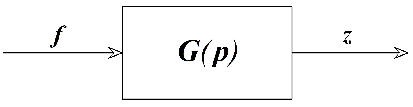
4. Definition of System Output and Optimization Goal
4.1. Any Component of the State Vector x
4.2. Any Component of the Strain and Stress Tensors
4.3. The Structural Compliance
- any coincides with a proper component of the state vector x;
- to any load , a compliance is associated that is defined as ;
- the overall compliance is defined as .
4.3.1. SISO Case
4.3.2. MISO Case
4.3.3. SIMO Case
4.3.4. MIMO Case
5. Implementation Details Using MATLAB
- main_stat.m is the main file of the project, containing all user-defined parameters of MMTO algorithm and case study. Once their are properly setup, main_stat.m calls three further scripts, namely initialize_mma.m, which contains the parameters of the MMA algorithm, start_mma.m, which solves the MMTO problem using the MMA algorithm, and plot_densities.m, which takes care of producing the figures displayed in this paper.
- The casestudy folder contains the code required to define the setup of the case study, including the definition of loads (defineLoads.m), the definition of supports (defineSupports.m), and the computation of the dynamic system matrices B and C (prepareDynamicSystemSS_BandC.m).
- The costandconstraints folder contains the code required to define the objective function and the constraints of the MMTO problem. Specifically, the function compliance_stat_mma.m calls two dedicated subroutines to evaluate the objective function and its derivatives (computeCostWithSensitivities.m), and evaluate constraint violations and their derivatives (computeConstraintsWithSensitivities.m) at the current guess for the MMTO problem.
- The filteringprojectioninterpolation folder contains the code implementing the filtering, projection and interpolation functions for Multi-Materials, as discussed in Section 2.
- The matrixnorms folder contains the code required to carry out the computation of tensor norms (pnormmat.m and pnormmatmenouno.m) and their derivatives (pnormmatsens.m), as discussed in Section 3.
- The stiffnesscomputations folder contains the code required to compute the stiffness matrix of the system, based on the desired finite element discretization, relying on the subroutines prepareStiffnessMatIdxs.m, prepareFEM.m and computeStiffnessMatrix.m.
- The MMA folder contains the code of the MMA algorithm, as made available by [23].
- The utils folder contains the computeDependentParams.m function, which computes additional parameters of the MMTO algorithm, based on the user-defined parameters set in main_stat.m.
6. Numerical Results
- a simply supported cantilevered beam;
- an L-shaped appended structure.
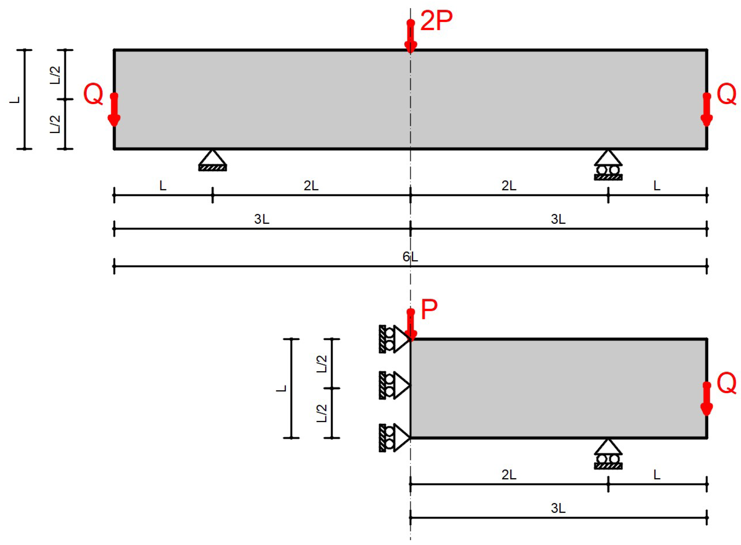
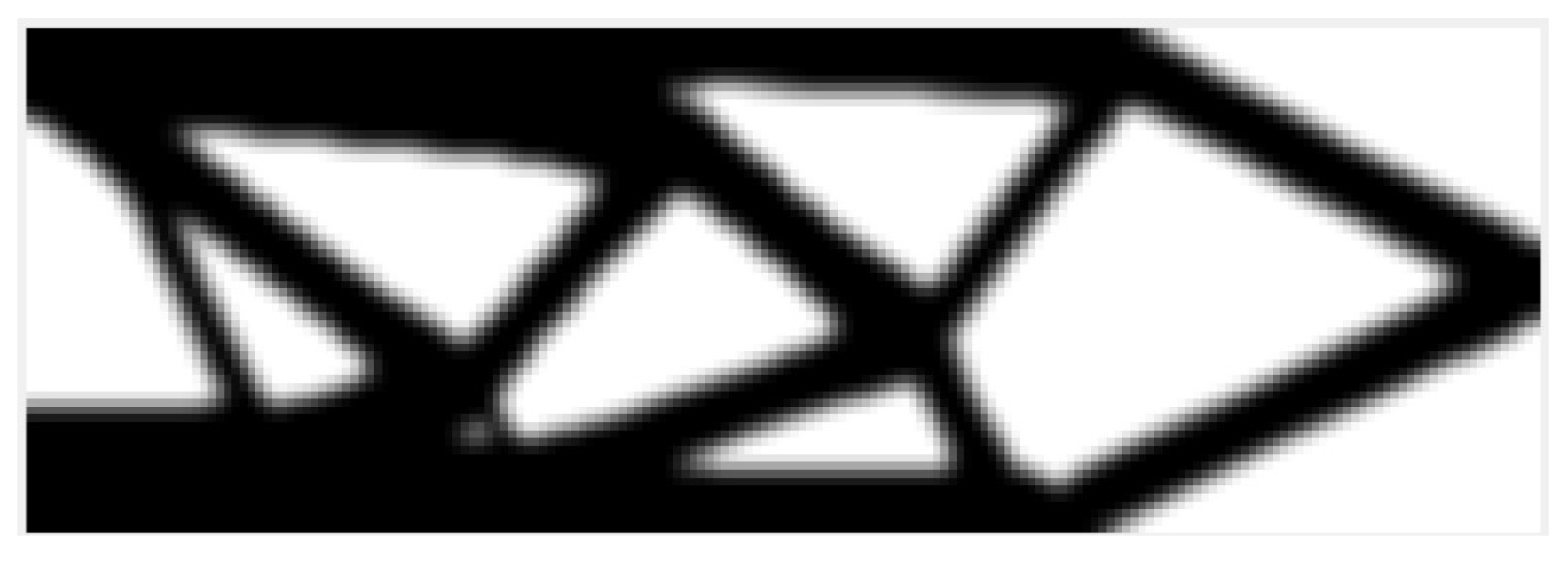
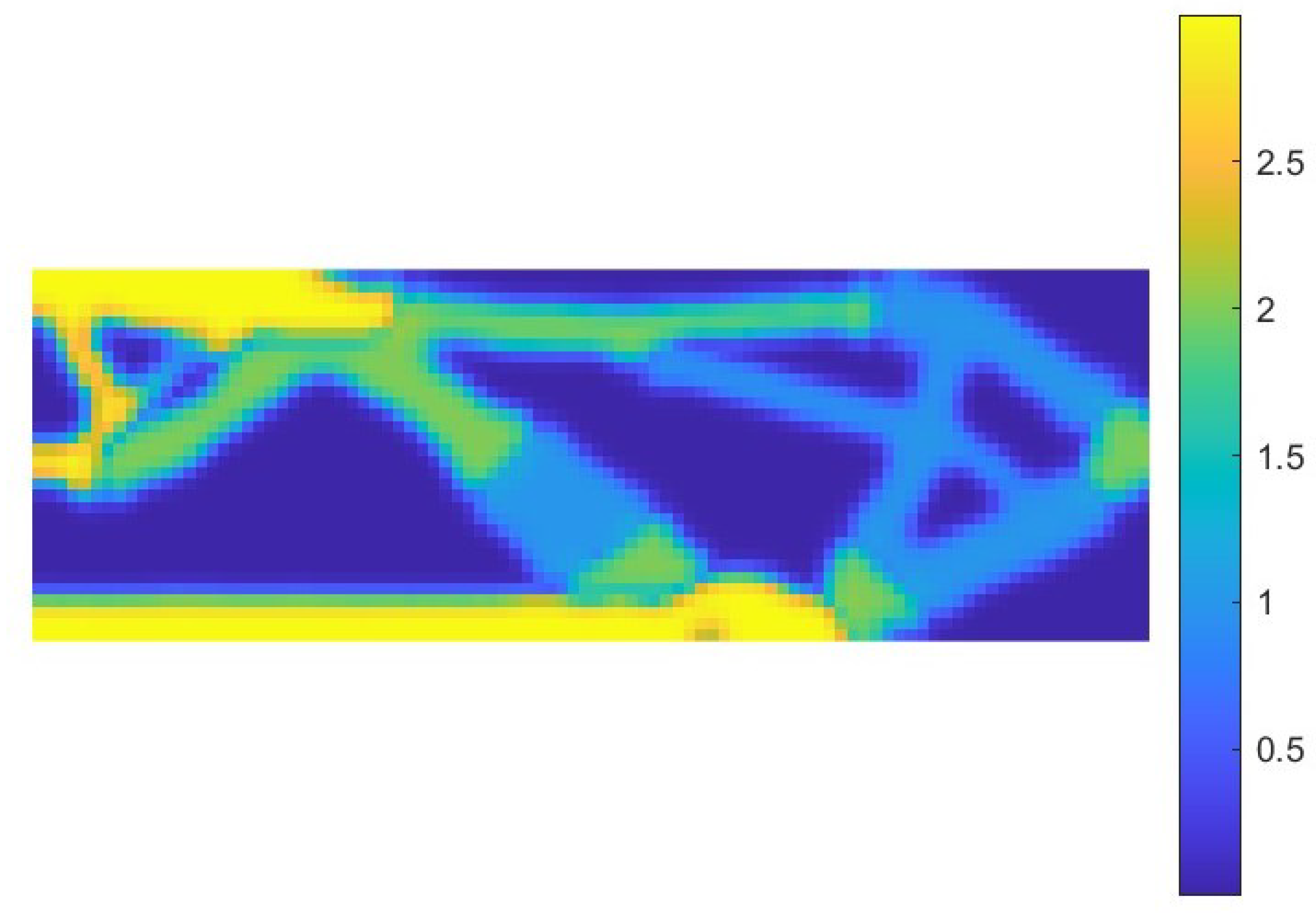
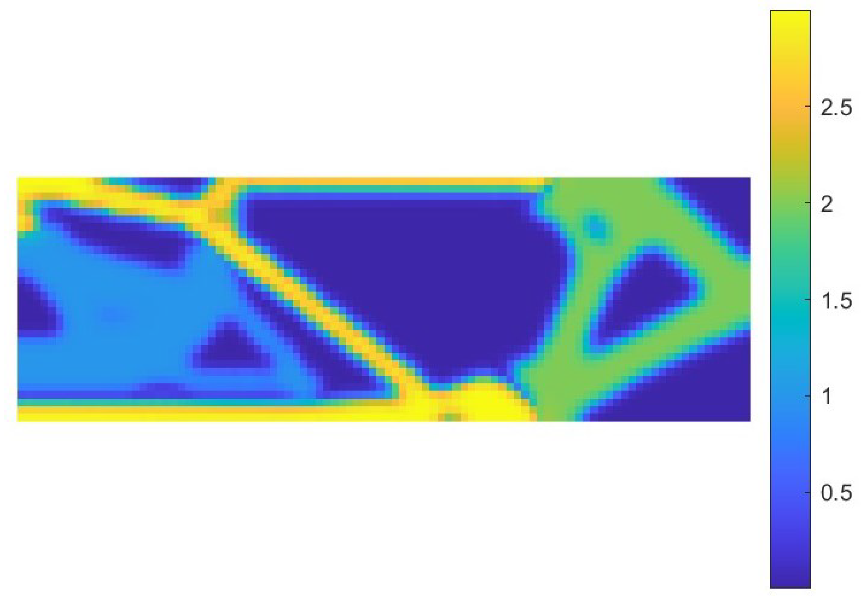
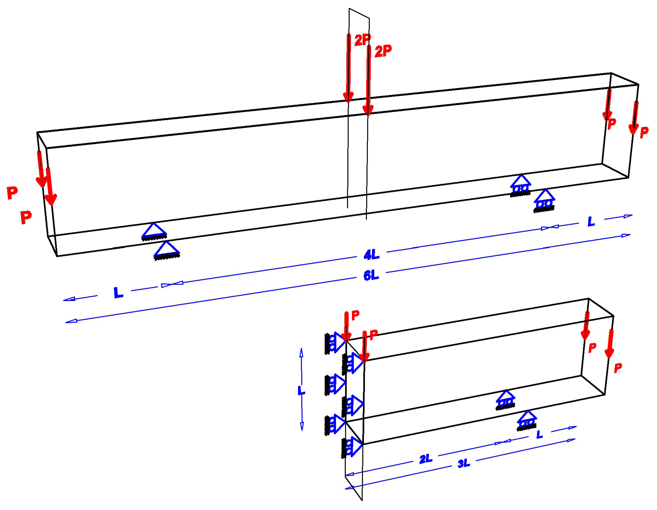
6.1. Simply Supported Cantilevered Beam
6.1.1. General Data
- -
- Poisson ratio: ;
- -
- Number of elements in vertical (Y) direction: ;
- -
- Number of elements in horizontal (X) direction: ;
- -
- Side length: (by this choice a uniform mesh of square elements of unit size is generated);
- -
- ;
- -
- Volume fraction = 0.5;
- -
- SIMP penalization factor: n = 3;
- -
- p-norm parameter = 6;
- -
- .
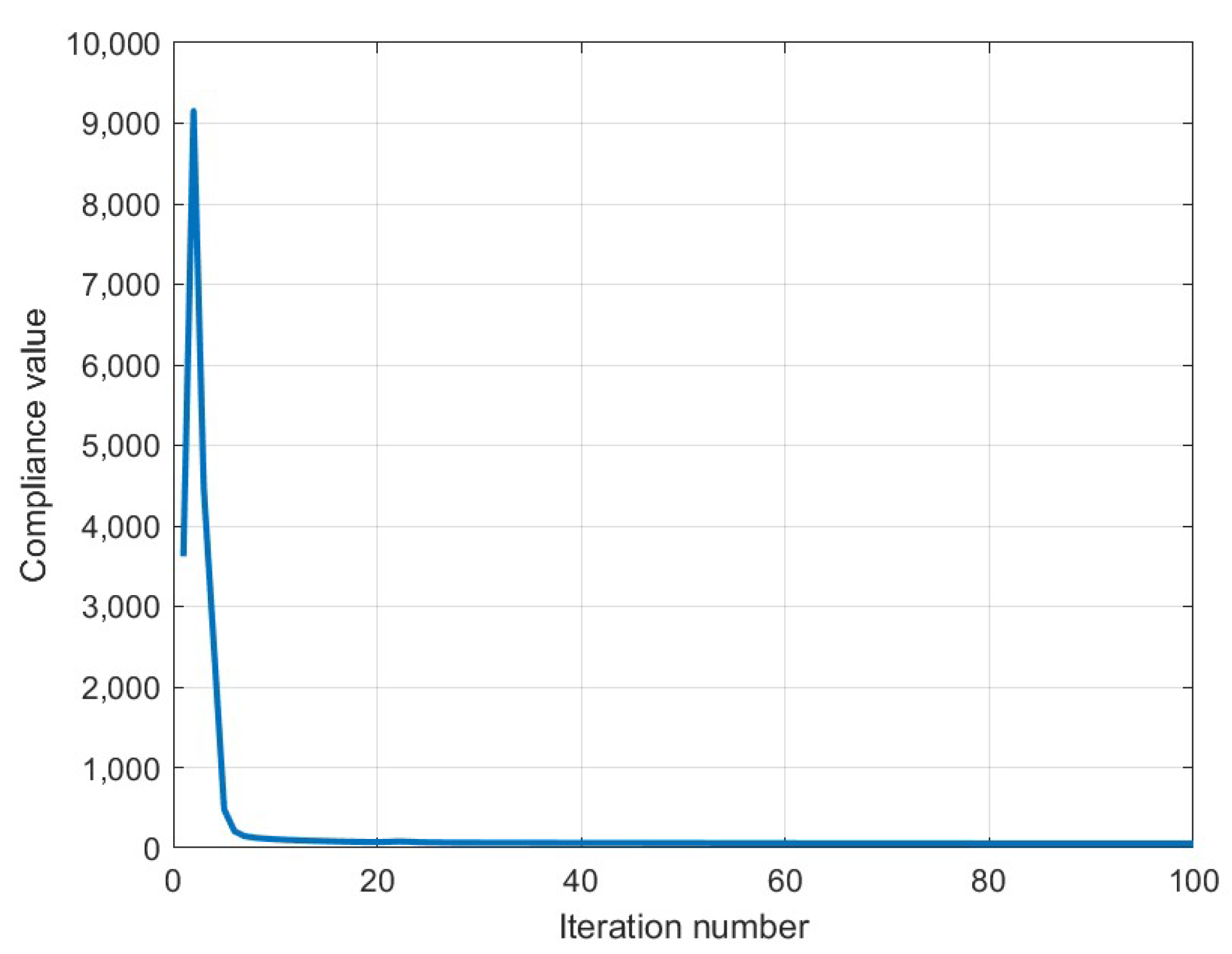
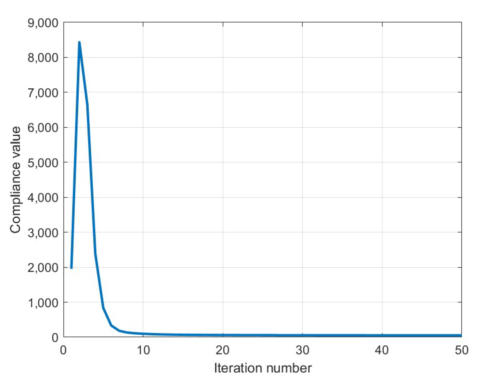
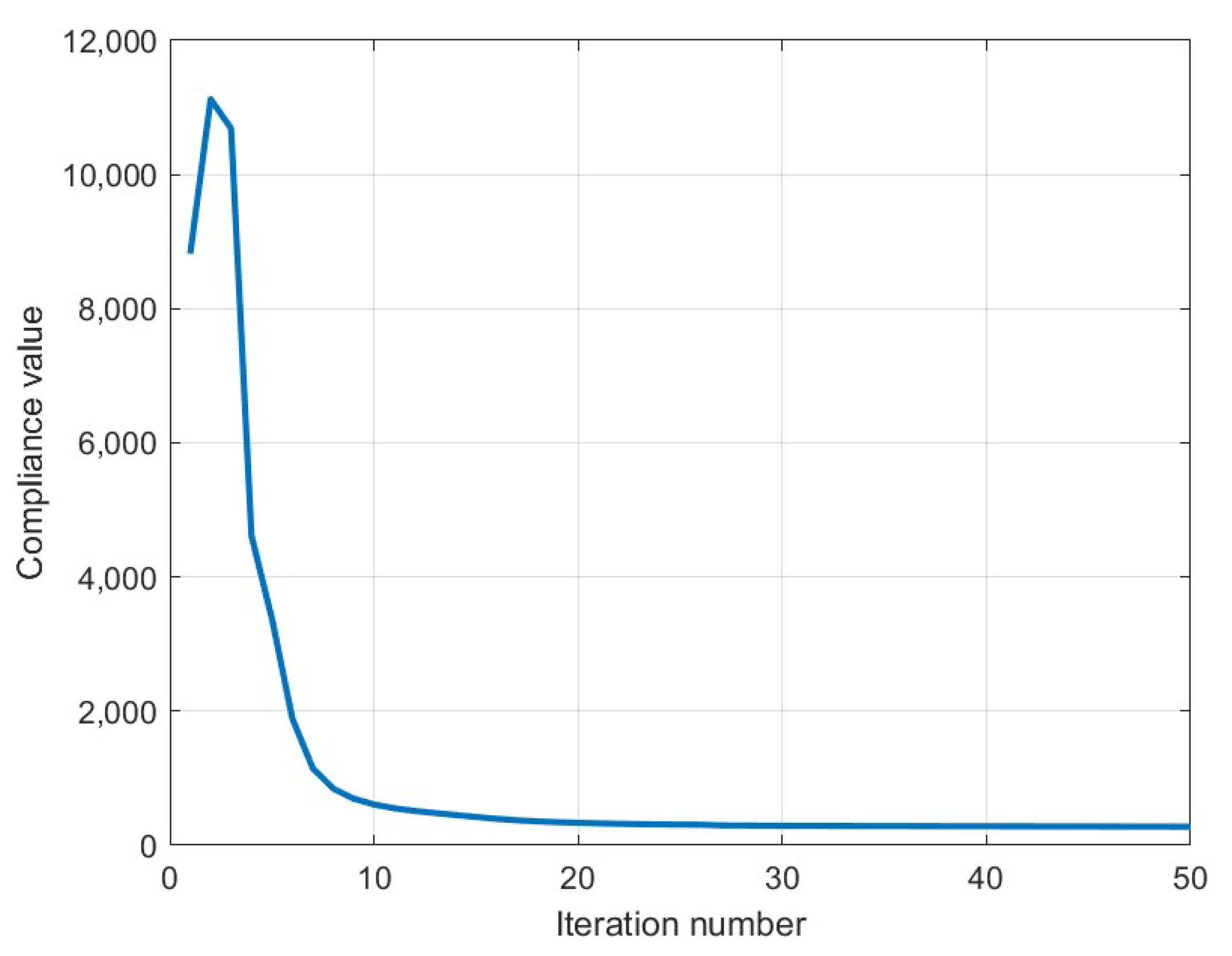
6.1.2. SISO System
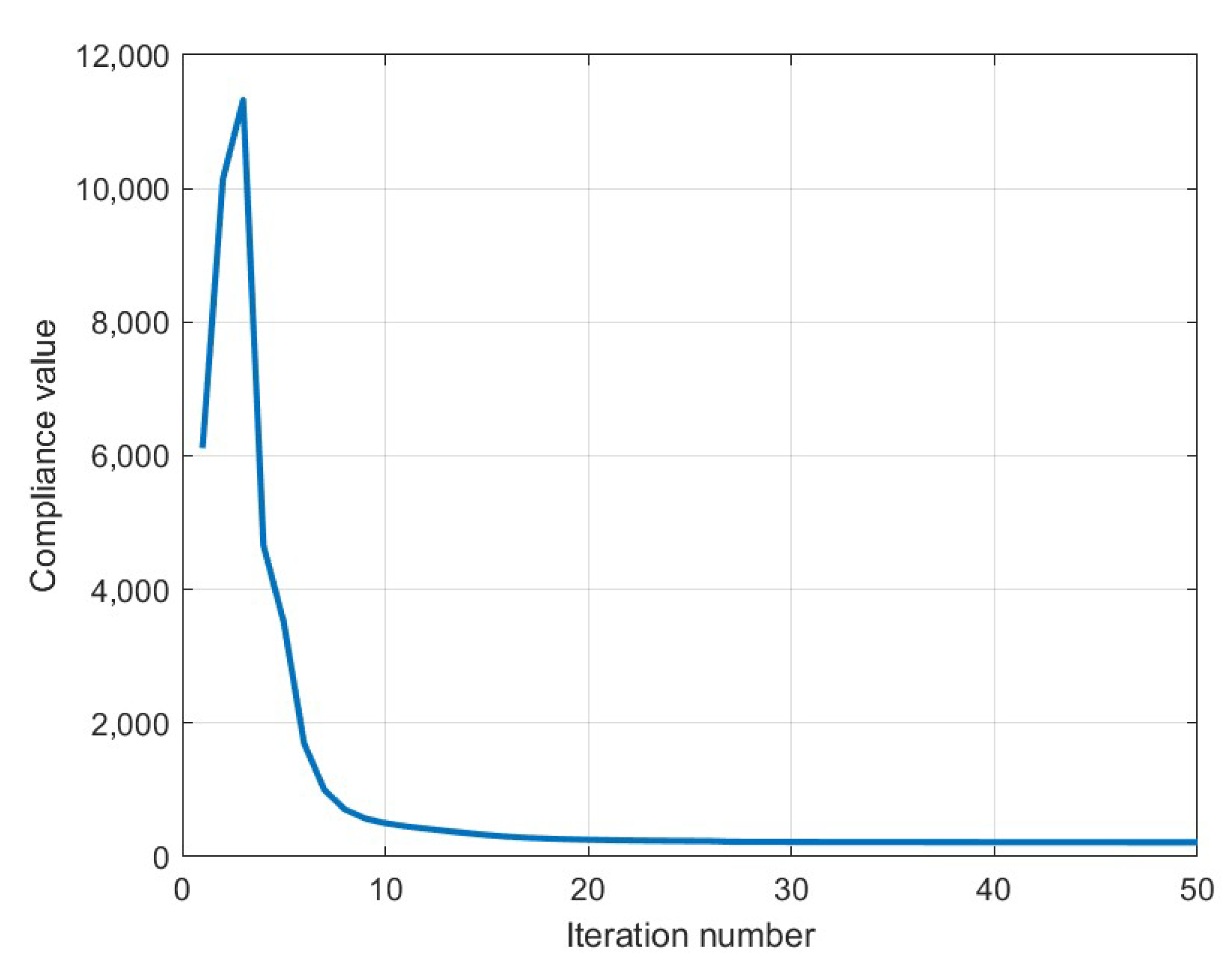
6.1.3. Stability of the Results with Respect to Mesh Resolution: A Trade-Off with Computational Cost
- On one hand, the numerical method may be sensitive to the level of discretization, implying that accurate and reliable solutions can only be achieved with sufficiently fine meshes.
- On the other hand, finer meshes enable a richer representation of the design space, allowing for a broader range of topologies to be captured as the continuous, infinite-dimensional domain is projected onto its discrete, finite-dimensional counterpart.
- 1.
- Number of elements in Y direction = 16; number of elements in X direction = 48;
- 2.
- Number of elements in Y direction = 32; number of elements in X direction = 96;
- 3.
- Number of elements in Y direction = 64; number of elements in X direction = 192;
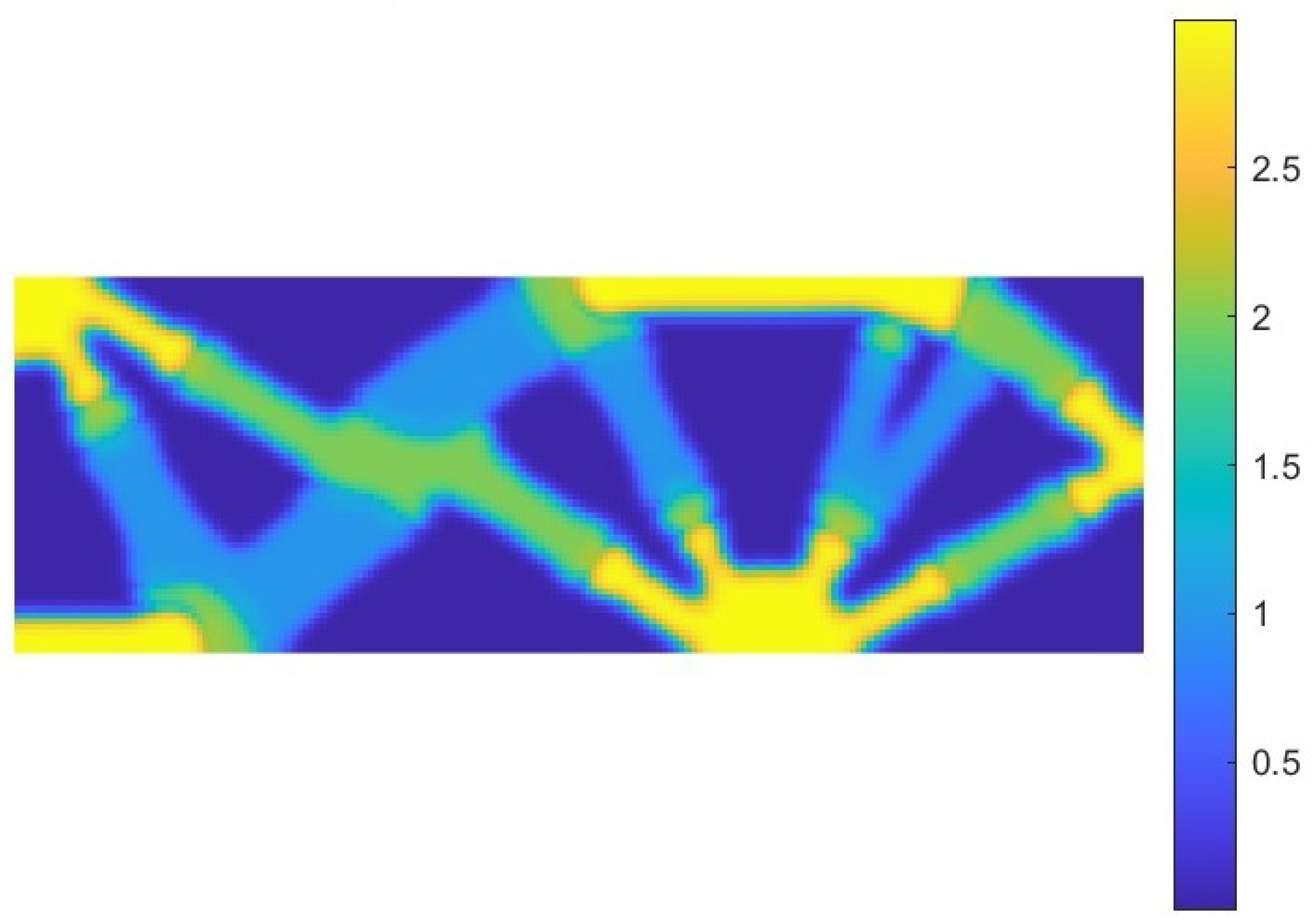
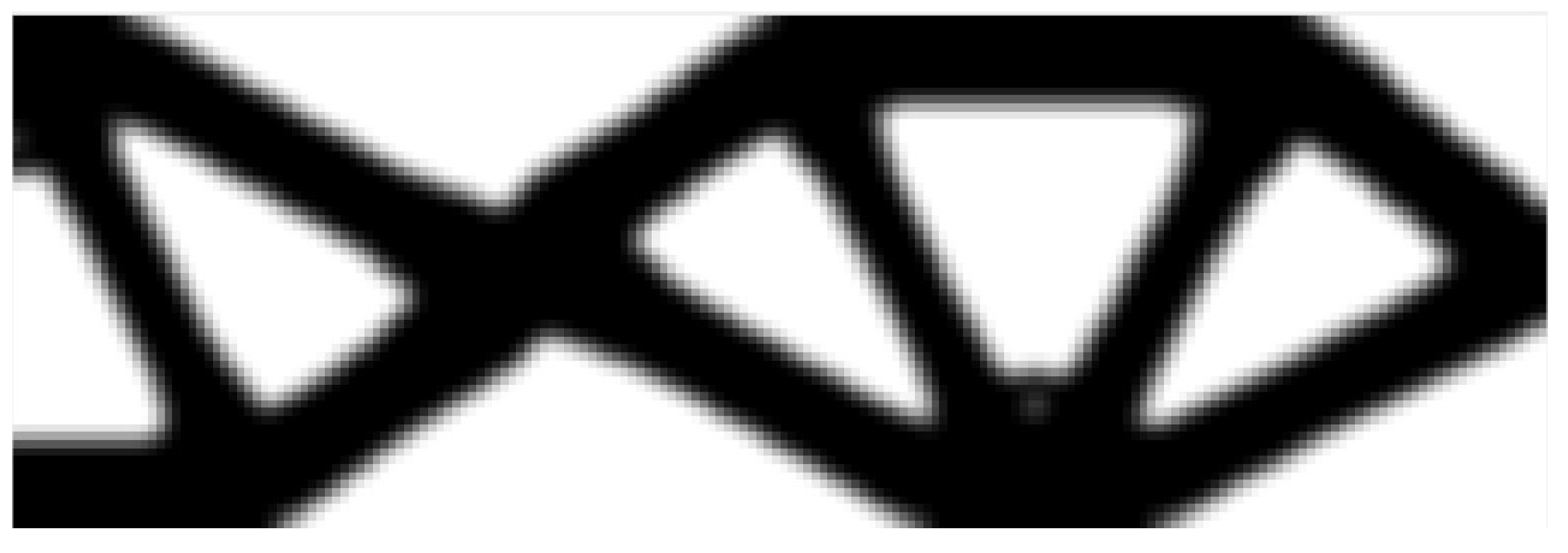
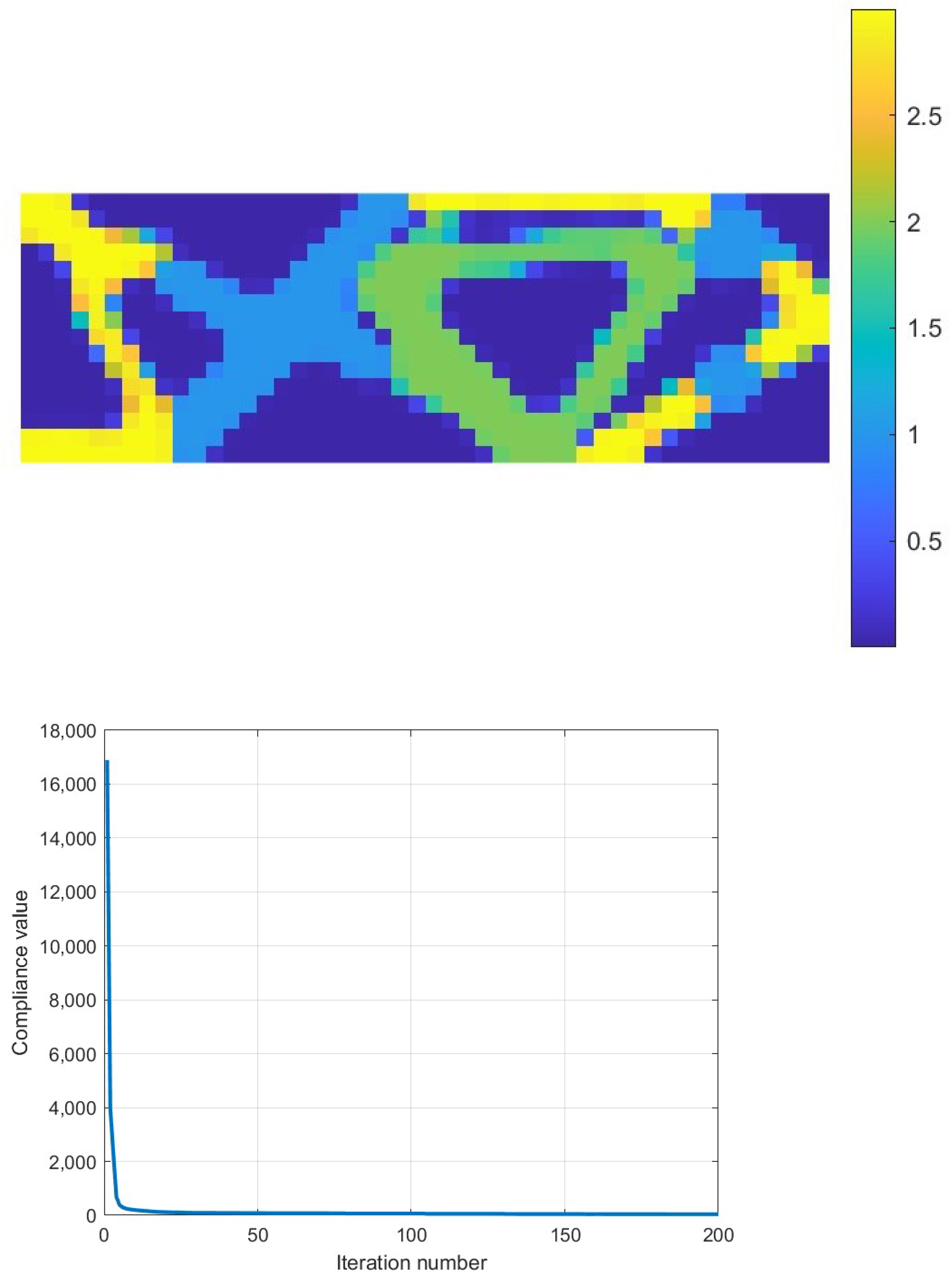
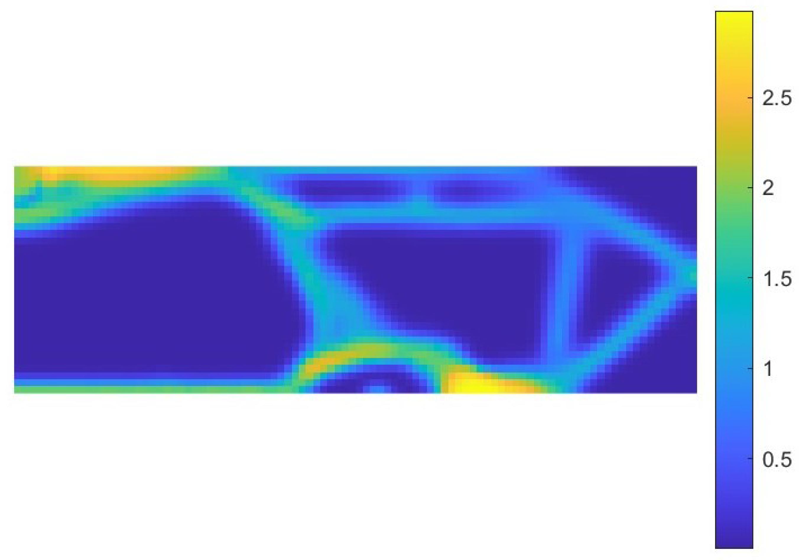
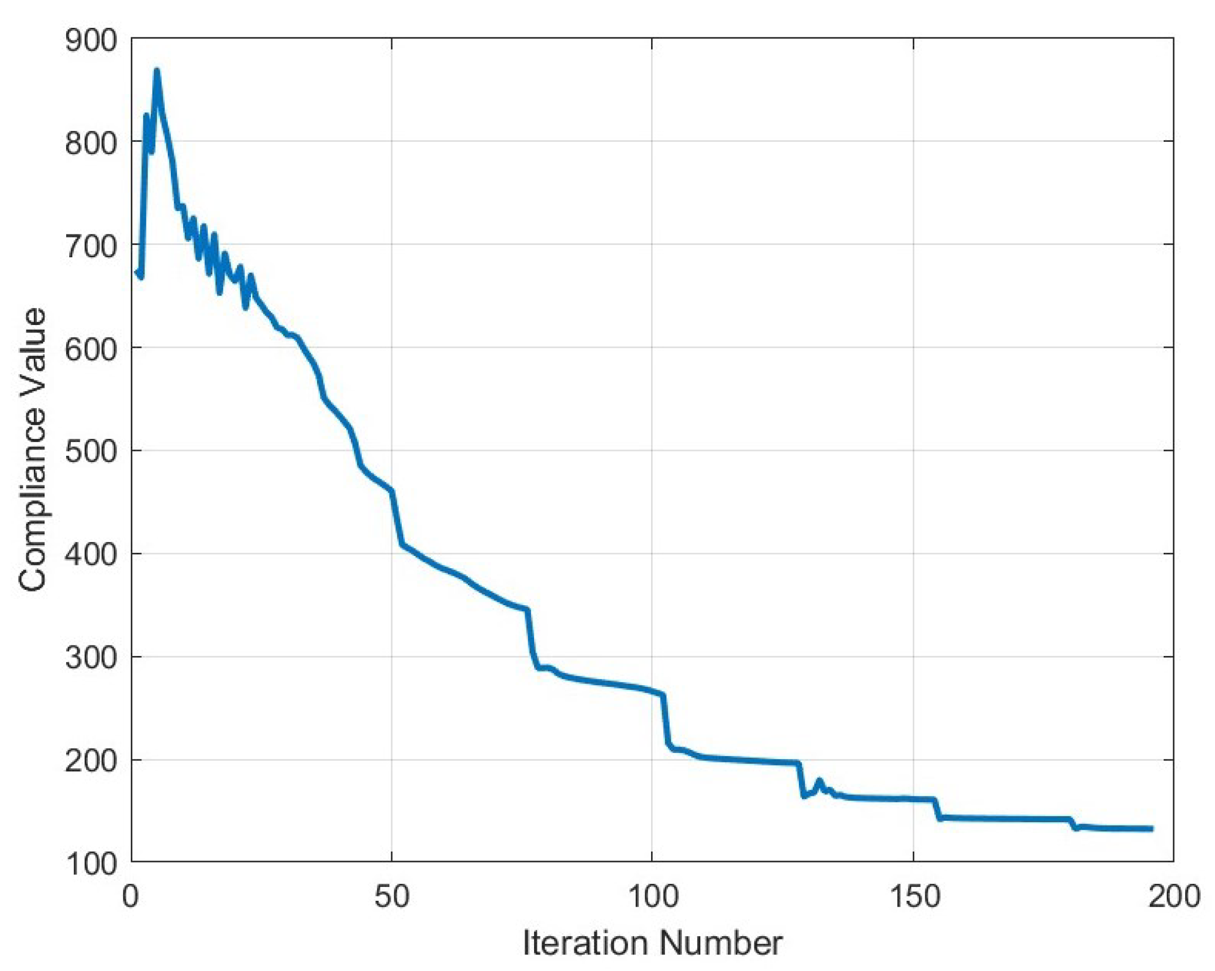
6.1.4. MIMO System-Norm 2
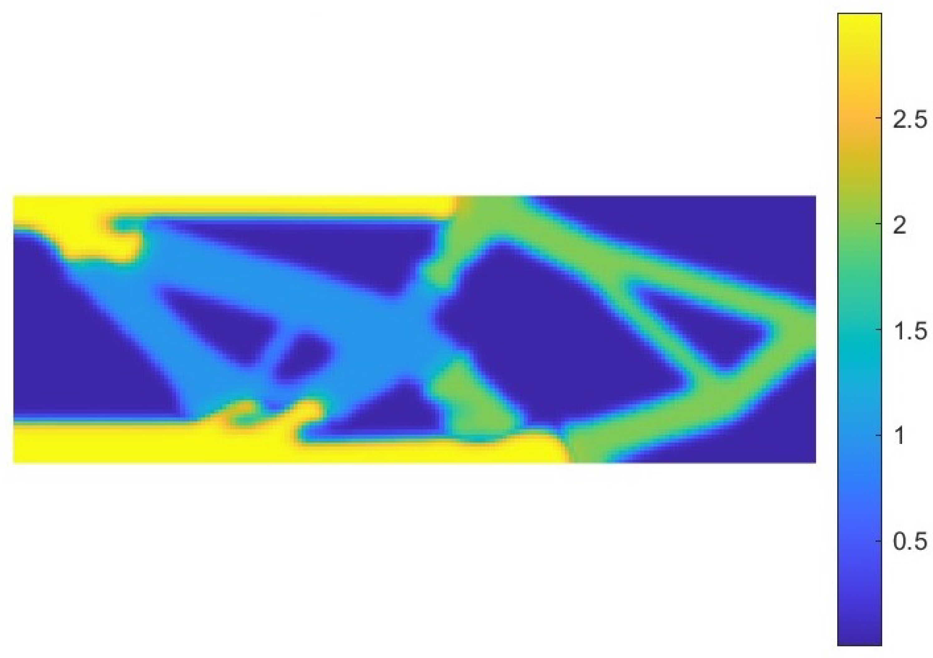
6.1.5. Effect of the SIMP Penalization Factor n on the Optimal Topology
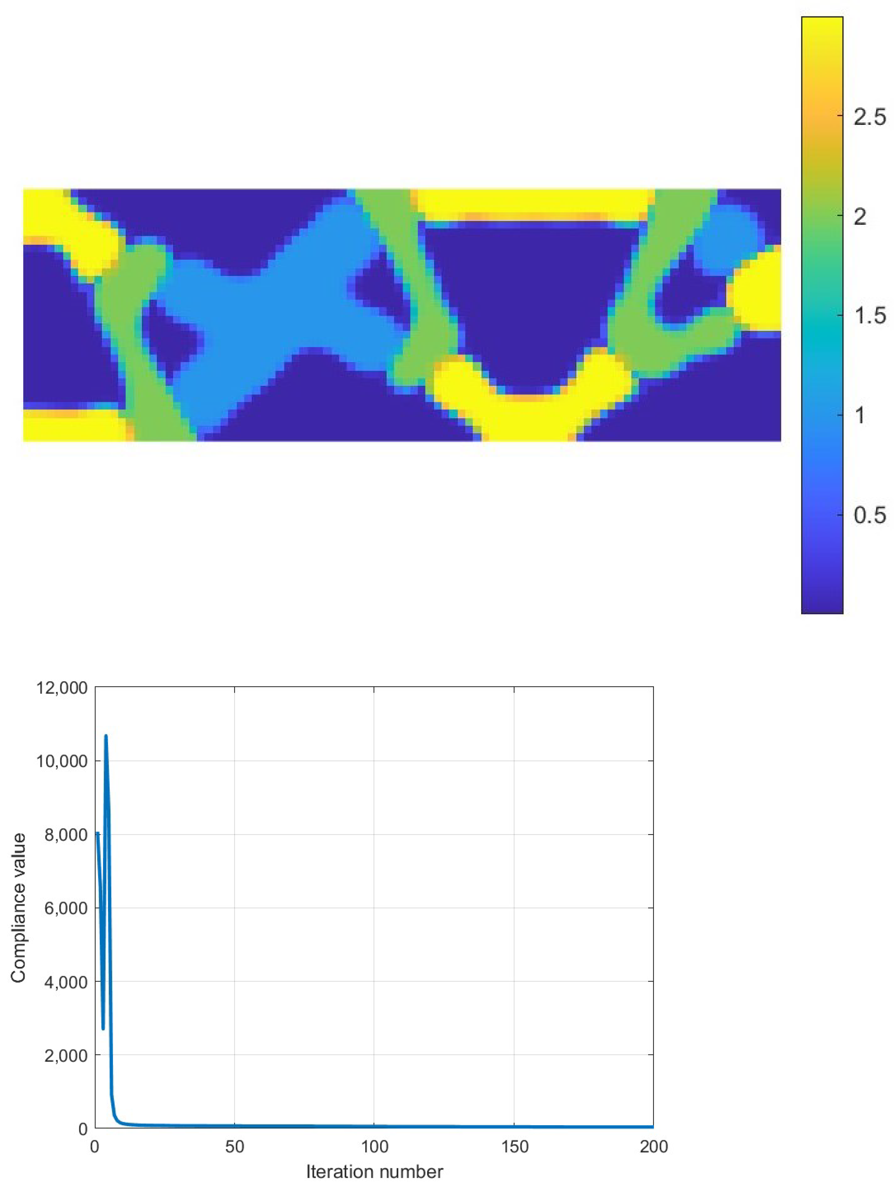
6.1.6. MIMO System-Nuclear Norm
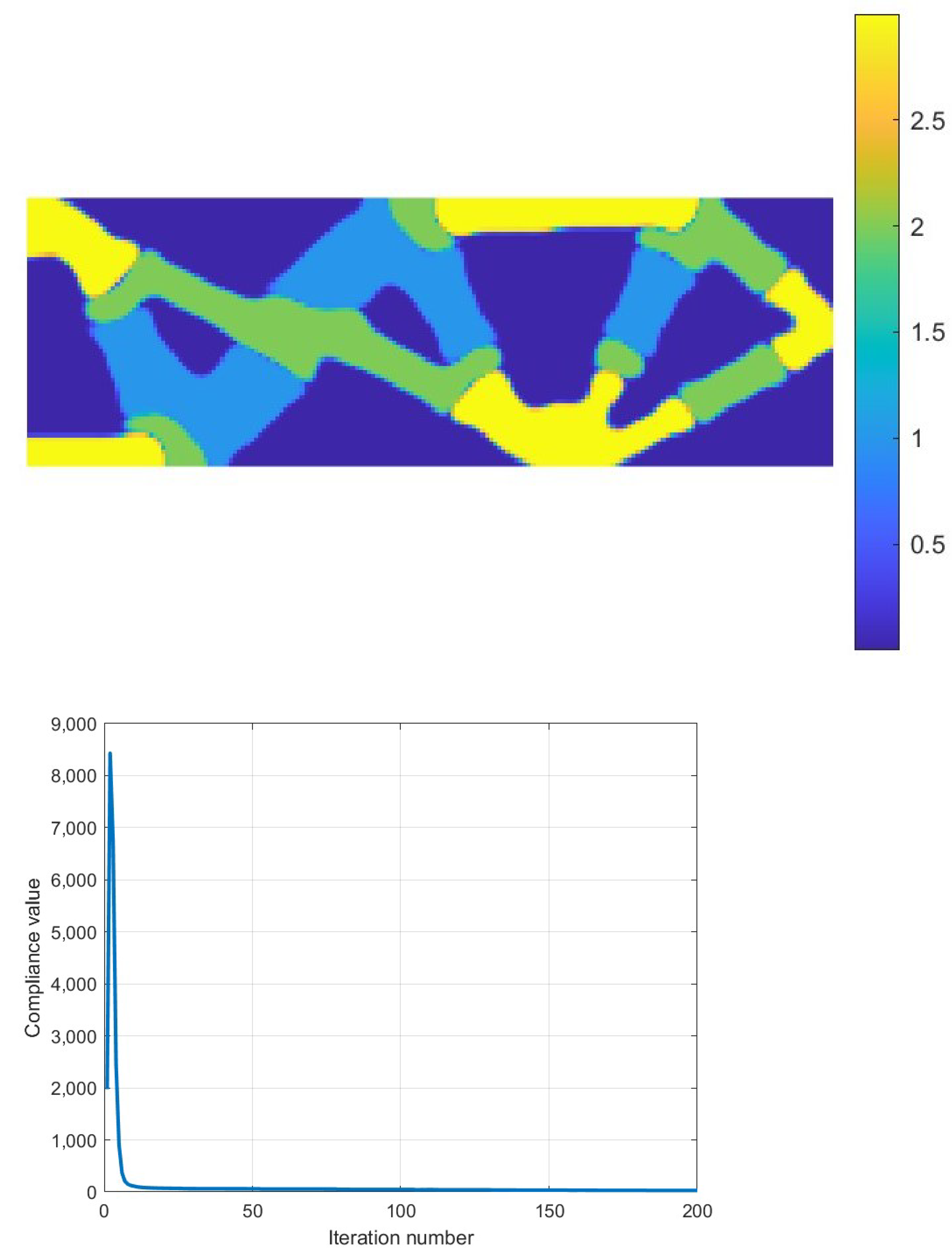
6.1.7. MIMO System-Frobenius Norm
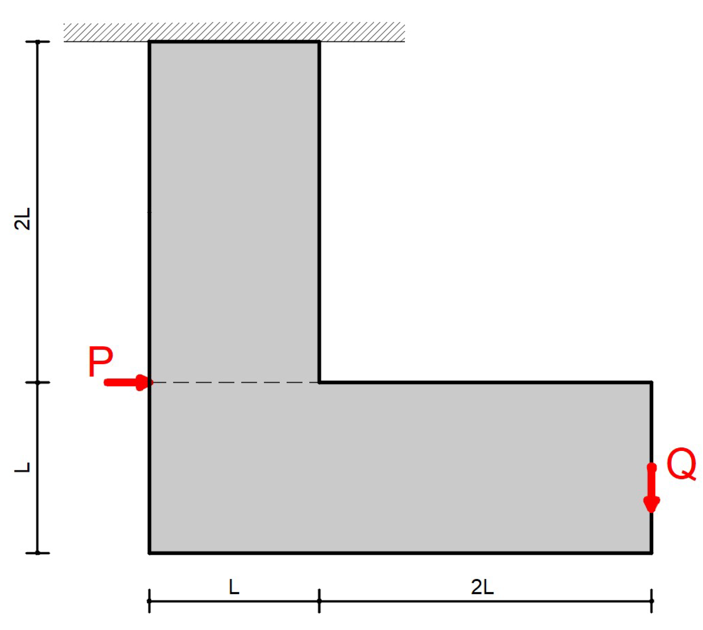
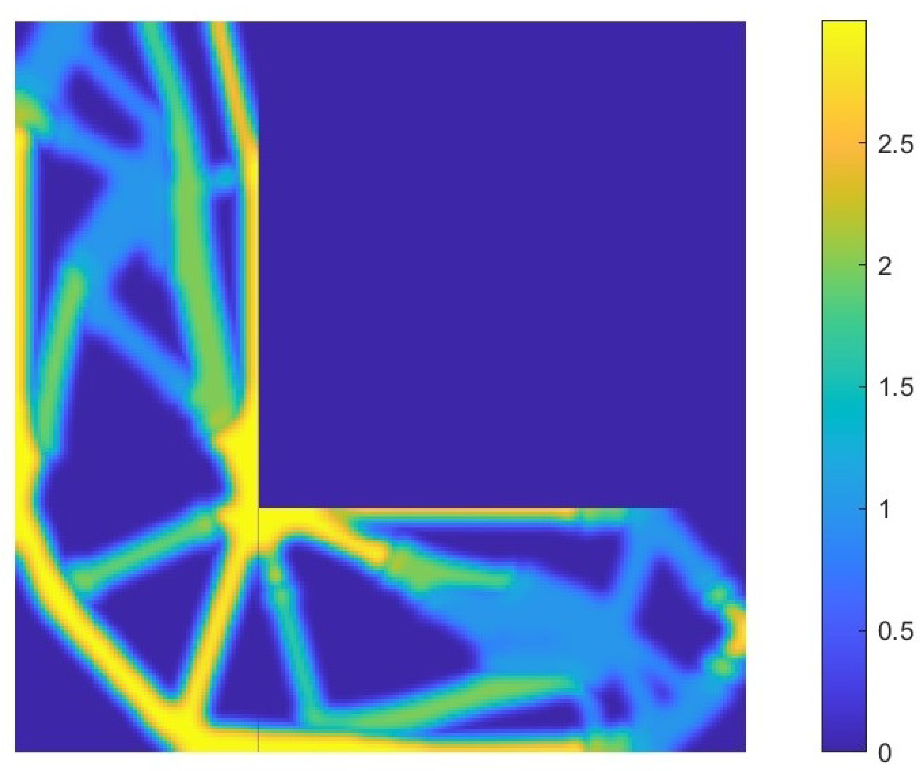
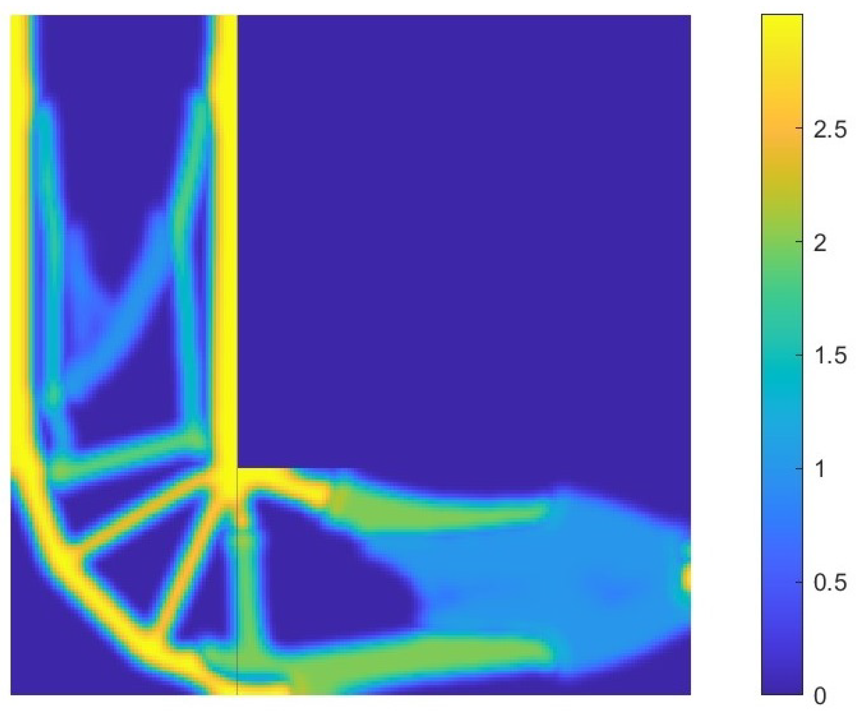
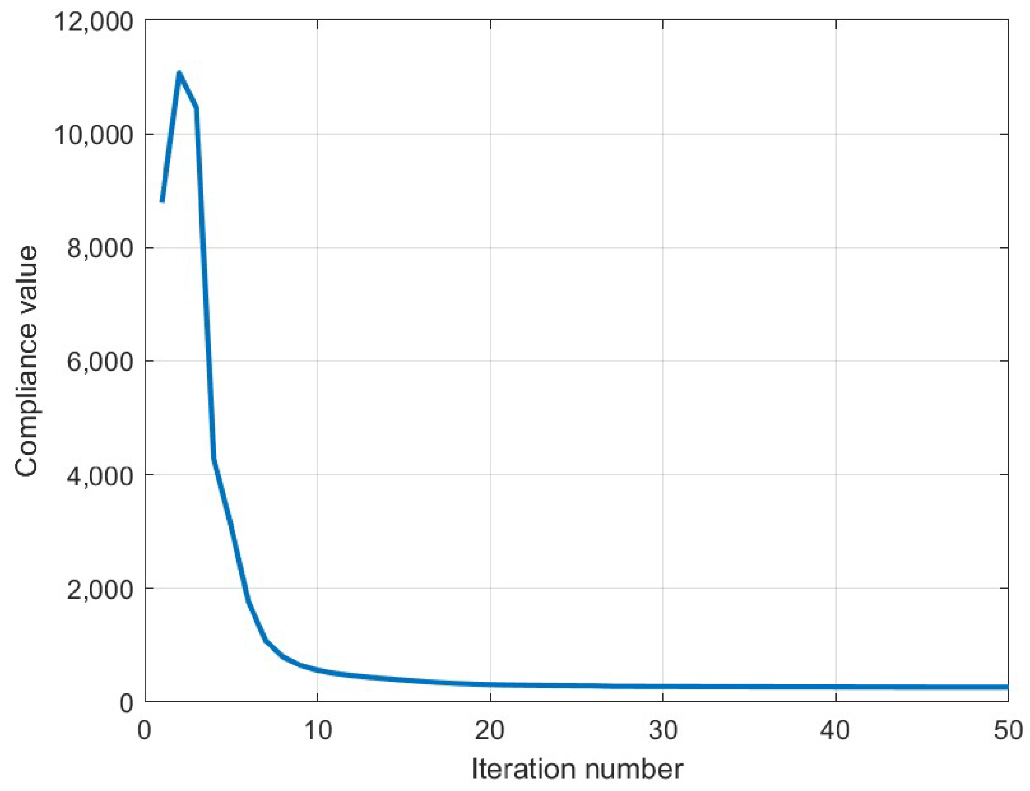
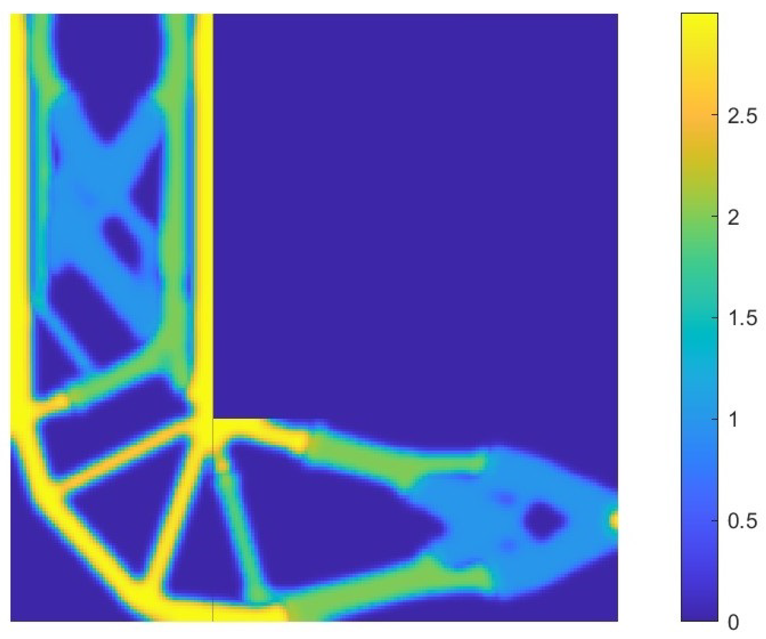
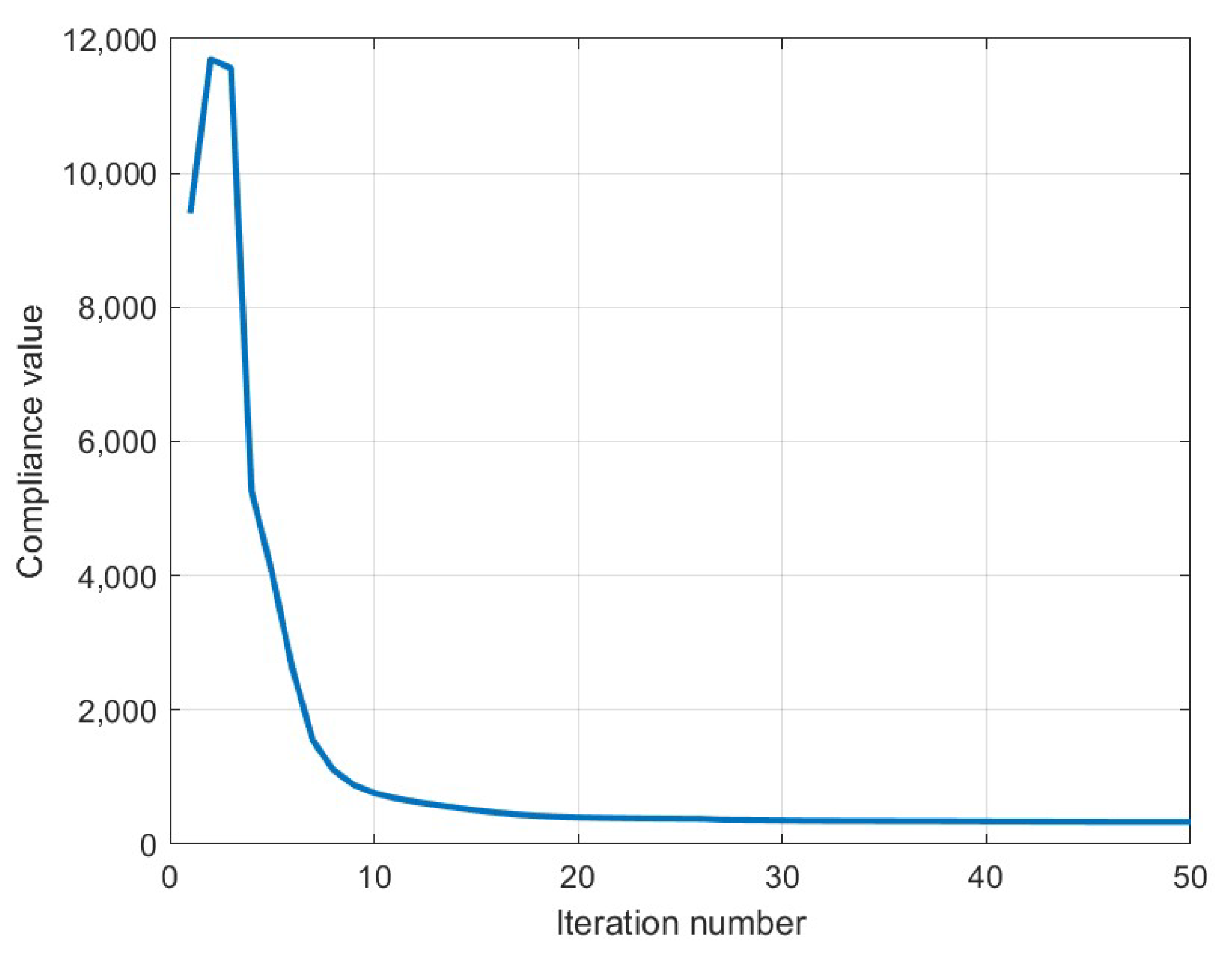
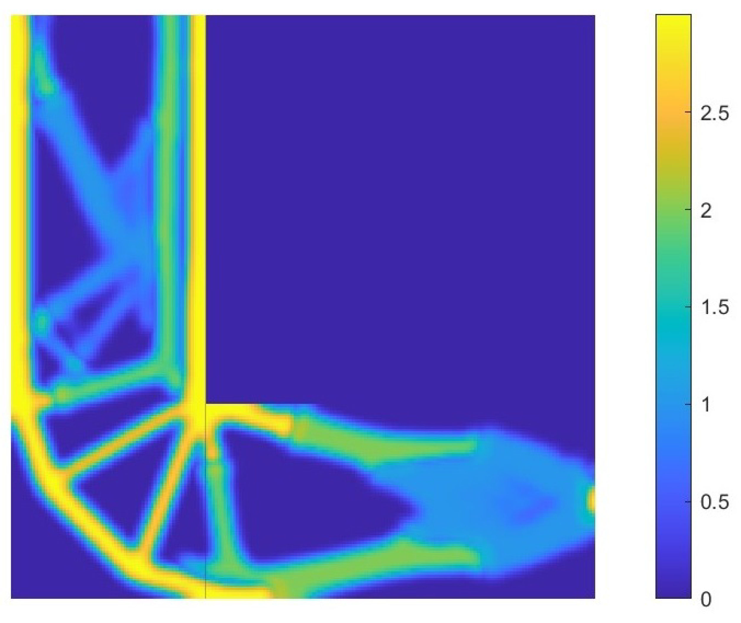
6.2. L-Shaped Structure
- -
- Poisson ratio: ;
- -
- Number of elements in vertical (Y) direction: ;
- -
- Number of elements in horizontal (X) direction: ;
- -
- Side length: ;
- -
- ;
- -
- Volume fraction = 0.5;
- -
- SIMP penalization factor: n = 3;
- -
- p-norm parameter = 6;
- -
- .
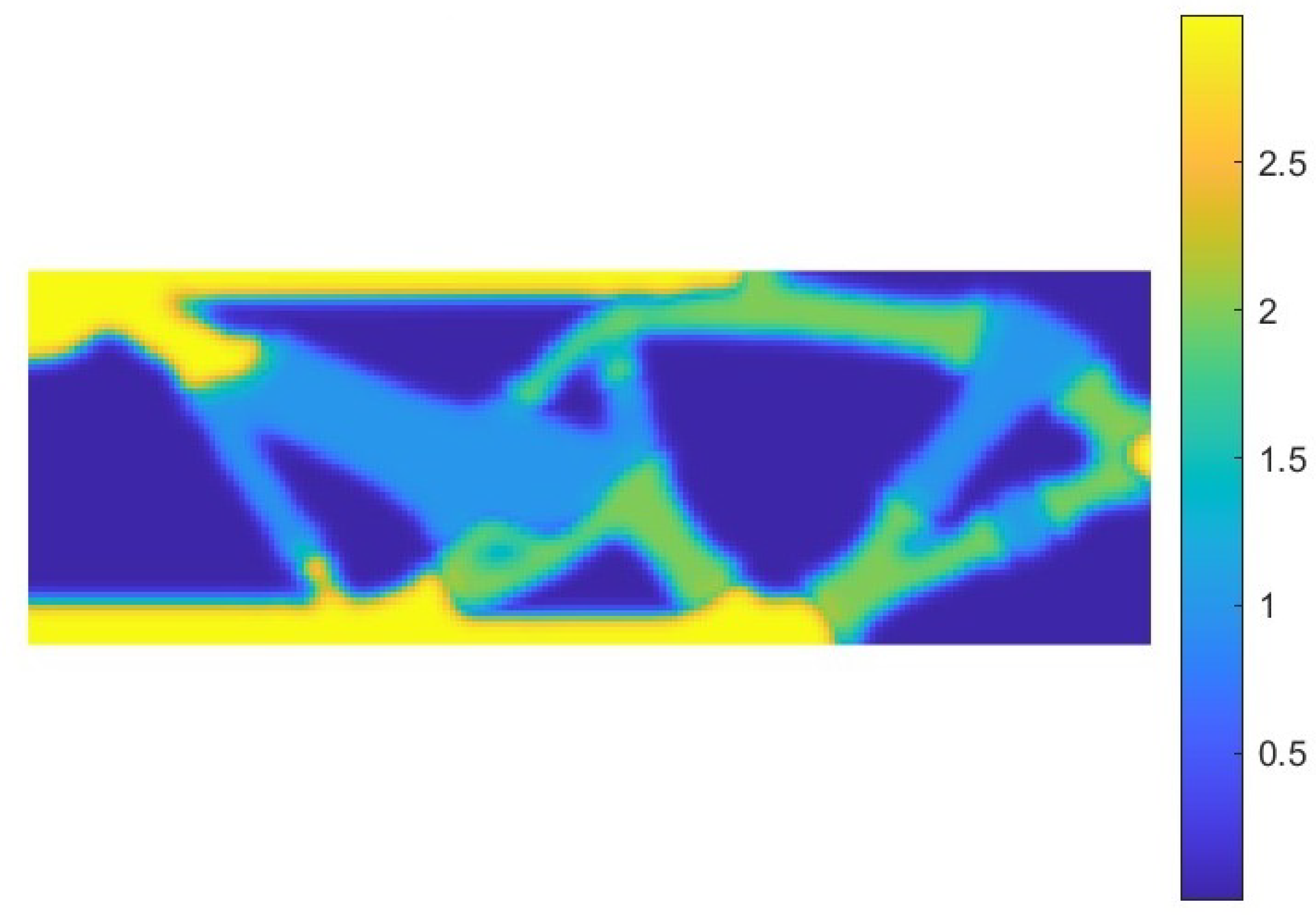
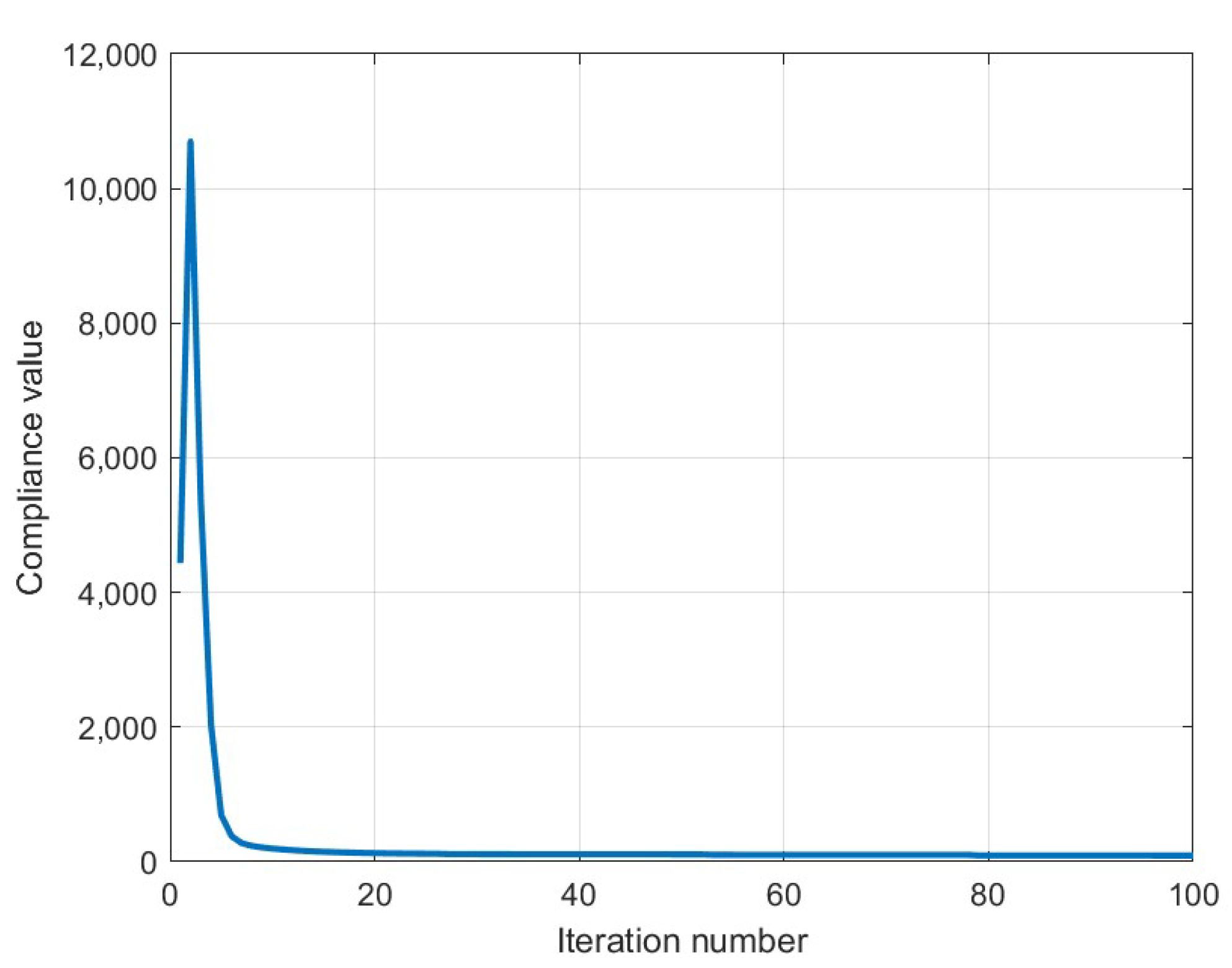
6.2.1. SISO System
6.2.2. MIMO System-2 Norm
6.2.3. MIMO System-Nuclear Norm
6.2.4. MIMO System-Frobenius Norm
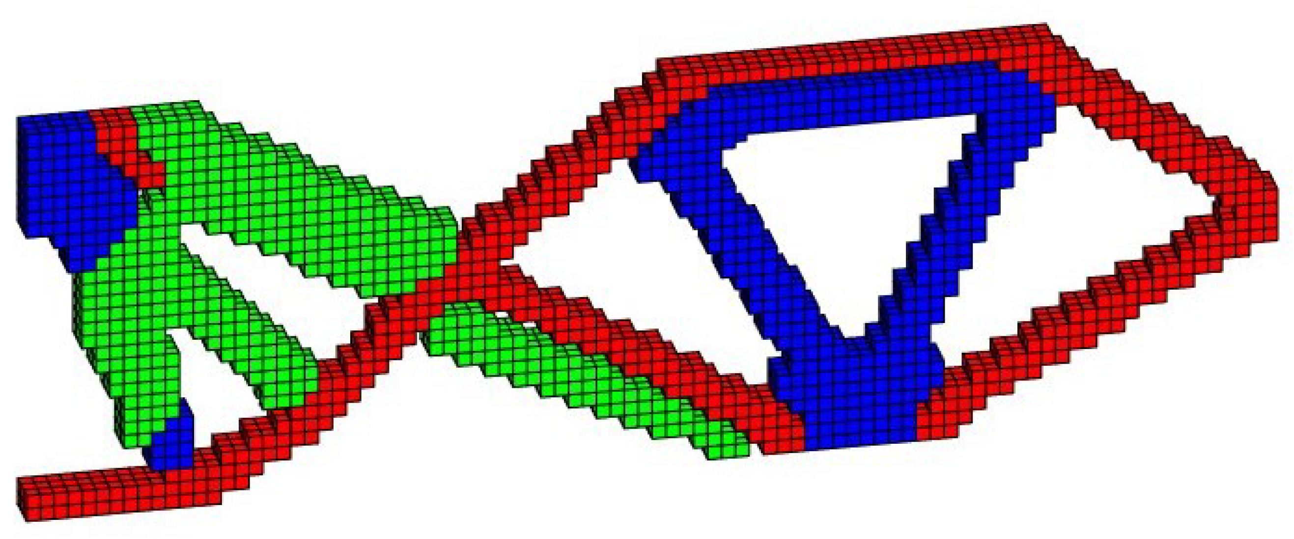
6.3. 3D Problem
- -
- Number of elements in the transverse (Y) direction: 30;
- -
- Number of elements in the longitudinal (X) direction: 90;
- -
- Number of elements in the vertical, top-down (Z) direction: 3;
- -
- SIMP penalization factor: 3;
- -
- p-norm parameter: 6;
- -
- Filter distance: ;
- -
- Initial value of the filter parameter: ;
- -
- ;
- -
- Number of materials: 3;
- -
- Young moduli: , , ;
- -
- Poisson ratio: .
7. Conclusions
Author Contributions
Funding
Data Availability Statement
Conflicts of Interest
References
- Bendsøe, M.; Kikuchi, N. Generating optimal topologies in structural design using a homogenization method. Comput. Methods Appl. Mech. Eng. 1988, 71, 197–224. [Google Scholar] [CrossRef]
- Sigmund, O. A 99 line topology optimization code written in Matlab. Struct. Multidiscip. Optim. 2001, 21, 120–127. [Google Scholar] [CrossRef]
- Zuo, K.; Saitou, K. Ordered SIMP interpolation for multi-material topology optimization. Struct. Multidiscip. Optim. 2017, 55, 477–491. [Google Scholar]
- Ogawa, S.; Yonekura, K.; Suzuki, K. Multimaterial topology optimization of unsteady heat conduction problems based on discrete material optimization. Int. J. Heat Mass Transf. 2024, 225, 125353. [Google Scholar] [CrossRef]
- Yin, L.; Ananthasuresh, G. Topology optimization of compliant mechanisms with multiple materials using a peak function material interpolation scheme. Struct. Multidiscip. Optim. 2006, 33, 199–214. [Google Scholar] [CrossRef]
- Zheng, R.; Yi, B.; Peng, X.; Yoon, G.H. An Efficient Code for the Multi-Material Topology Optimization of 2D/3D Continuum Structures Written in Matlab. Appl. Sci. 2024, 14, 657. [Google Scholar] [CrossRef]
- Andreassen, E.; Clausen, A.; Schevenels, M.; Lazarov, B.S.; Sigmund, O. Efficient topology optimization in MATLAB using 88 lines of code. Struct. Multidiscip. Optim. 2011, 43, 1–16. [Google Scholar] [CrossRef]
- Dinh, T.; Hedayatrasa, S.; Bormann, F.; Bosman, M.; Paepegem, W.V. A smooth single-variable-based interpolation function for multi-material topology optimization. Eng. Comput. 2024, 40, 2841–2855. [Google Scholar] [CrossRef]
- Asadpoure, A.; Rahman, M.; Nejat, S.; Javidannia, L.; Valdevit, L.; Guest, J.; Tootkaboni, M. Topology optimization with multi-phase length-scale control. Int. J. Mech. Sci. 2025, 291–292, 110086. [Google Scholar] [CrossRef]
- Jia, Y.; Li, W.; Zhang, X. Multimaterial topology optimization of elastoplastic composite structures. J. Mech. Phys. Solids 2025, 196, 106018. [Google Scholar] [CrossRef]
- Hvejsel, C.; Lund, E. Material interpolation schemes in topology optimization. Int. J. Numer. Methods Eng. 2011, 85, 575–599. [Google Scholar]
- Bruyneel, M. A general and efficient multi-material topology optimization approach using the shape function with penalization. Struct. Multidiscip. Optim. 2010, 42, 529–553. [Google Scholar]
- Huang, X.D.; Xie, Y.M. Bi-directional evolutionary structural optimization with buckling constraints. Struct. Multidiscip. Optim. 2023, 67, 123–135. [Google Scholar]
- Huang, X. Smooth topological design of structures using the floating projection. Eng. Struct. 2020, 208, 110330. [Google Scholar] [CrossRef]
- Huang, X.D.; Li, W. Three-field floating projection topology optimization of continuum structures. Comput. Methods Appl. Mech. Eng. 2022, 398, 115259. [Google Scholar] [CrossRef]
- Fu, Y.F.; Rolfe, B.; Chiu, N.S.L.; Wang, Y.; Huang, X.; Ghabraie, K. Smooth-edged material distribution for optimizing topology algorithm. Adv. Eng. Softw. 2020, 149, 102921. [Google Scholar] [CrossRef]
- Sanders, E.D.; Pereira, A.; Aguiló, M.A.; Paulino, G.H. PolyMat: An efficient Matlab code for multi-material topology optimization. Struct. Multidiscip. Optim. 2018, 58, 2727–2759. [Google Scholar] [CrossRef]
- Brunton, S.; Kutz, J. Data-Driven Science and Engineering—Machine Learning, Dynamical Systems and Control; Cambrige University Press: Cambridge, MA, USA, 2019. [Google Scholar]
- Strang, G. Linear Algebra and Learning from Data; Cambridge Press: Wellesley, MA, USA, 2019. [Google Scholar]
- Venini, P.; Pingaro, M. Static and dynamic topology optimization: An innovative unifying approach. Struct. Multidiscip. Optim. 2023, 66, 85. [Google Scholar] [CrossRef]
- Venini, P. A new rational approach to multi-input multi-output 3D topology optimization. Comput. Struct. 2024, 298, 107362. [Google Scholar] [CrossRef]
- Yi, B.; Yoon, G.; Zheng, R.; Liu, L.; Li, D.; Peng, X. A unified material interpolation for topology optimization of multi-materials. Comput. Struct. 2023, 282, 107041. [Google Scholar] [CrossRef]
- Svanberg, K. The method of moving asymptotes—A new method for structural optimization. Int. J. Numer. Methods Eng. 1987, 24, 359–373. [Google Scholar] [CrossRef]
- Lewis, A.S.; Overton, M.L. Eigenvalue optimization. Acta Numer. 1996, 5, 149–190. [Google Scholar] [CrossRef]
- Ehrgott, M. Multicriteria Optimization; Springer Science & Business Media: Berlin/Heidelberg, Germany, 2005. [Google Scholar]
- Bendsøe, M.P.; Sigmund, O. Material interpolation schemes in topology optimization. Arch. Appl. Mech. 1999, 69, 635–654. [Google Scholar] [CrossRef]
- Trefethen, L.N.; Bau, B. Numerical Linear Algebra; SIAM: Philadelphia, PA, USA, 1997. [Google Scholar]


| Compliance | 58.14 | 78.64 | 2451.72 |
Disclaimer/Publisher’s Note: The statements, opinions and data contained in all publications are solely those of the individual author(s) and contributor(s) and not of MDPI and/or the editor(s). MDPI and/or the editor(s) disclaim responsibility for any injury to people or property resulting from any ideas, methods, instructions or products referred to in the content. |
© 2025 by the authors. Licensee MDPI, Basel, Switzerland. This article is an open access article distributed under the terms and conditions of the Creative Commons Attribution (CC BY) license (https://creativecommons.org/licenses/by/4.0/).
Share and Cite
Galuppini, G.; Venini, P. A Transfer Matrix Norm-Based Framework for Multimaterial Topology Optimization: Methodology and MATLAB Implementation. Algorithms 2025, 18, 282. https://doi.org/10.3390/a18050282
Galuppini G, Venini P. A Transfer Matrix Norm-Based Framework for Multimaterial Topology Optimization: Methodology and MATLAB Implementation. Algorithms. 2025; 18(5):282. https://doi.org/10.3390/a18050282
Chicago/Turabian StyleGaluppini, Giacomo, and Paolo Venini. 2025. "A Transfer Matrix Norm-Based Framework for Multimaterial Topology Optimization: Methodology and MATLAB Implementation" Algorithms 18, no. 5: 282. https://doi.org/10.3390/a18050282
APA StyleGaluppini, G., & Venini, P. (2025). A Transfer Matrix Norm-Based Framework for Multimaterial Topology Optimization: Methodology and MATLAB Implementation. Algorithms, 18(5), 282. https://doi.org/10.3390/a18050282