1. Introduction
The minimum dominating set (MDS) problem is a fundamental optimization problem in graph theory, playing a crucial role in both theoretical computer science and practical applications [
1,
2]. For a graph
, a dominating set is a subset
such that every vertex
either belongs to
D or is adjacent to at least one vertex in
D. A minimum dominating set is a dominating set of minimum cardinality.
It is important to note that there is a significant difference between sequential algorithms, which process the entire graph with complete information, and distributed algorithms, which operate with limited local information at each node. In the context of solving the MDS problem, distributed algorithms that can be efficiently implemented in networks are particularly interesting. The LOCAL model, first introduced by Linial [
3], is one of the basic models of distributed computing, where a network is represented as a graph with vertices corresponding to processors and edges representing communication channels. In this model, in each round every vertex can send any message to all its neighbors, perform local computations, and receive messages from its neighbors. The complexity of an algorithm in the LOCAL model is measured by the number of communication rounds needed to solve the problem. An algorithm is called local if it operates in a constant number of rounds, regardless of the network size.
The computational complexity of the MDS problem has been studied in various computational models and for numerous graph classes. In general, the problem is NP-hard [
4], and, furthermore, finding an approximation with a factor of
for some constant
C is also NP-hard [
5].
A simple but effective greedy strategy achieves a logarithmic approximation ratio of
, where
n is the number of vertices in the graph [
6,
7]. Importantly, this approximation ratio is essentially the best possible for arbitrary graphs, as obtaining an approximation ratio better than
(for any
) is NP-hard [
8].
Researchers have sought restricted graph classes where better approximations are possible. For graph classes with subexponential expansion [
9], the problem admits a polynomial-time approximation scheme (PTAS). Constant-factor approximations exist for graphs with bounded degeneracy [
10,
11], bounded VC-dimension [
12,
13], and biclique-free graphs [
14] achieve an
approximation ratio.
For graphs with bounded arboricity, which includes planar and triangle-free planar graphs, significant results in sequential algorithms have been achieved. Bansal and Umboh [
15] provided a sequential algorithm achieving a
-approximation, where
d is the arboricity of the graph. Later, Dvořák [
16] improved this result to a
-approximation factor. Since planar triangle-free graphs have arboricity of at most 2, these results yield a sequential algorithm with an approximation factor of at most 5.
While these sequential algorithms achieve excellent approximation ratios, our focus in this paper is on distributed algorithms, which face the additional constraints of limited local information and communication requirements. In the distributed setting, Kuhn et al. [
17] proved lower bounds on the approximation of dominating sets depending on the number of communication rounds. Their results imply that constant-factor approximations essentially require
rounds. For specific graph classes, however, better results are possible.
For planar graphs, the MDS problem becomes more tractable. Czygrinow et al. [
18] achieved constant-factor approximations in
rounds on planar graphs. Lenzen et al. proposed a constant-round algorithm that computes a 130-approximation of the minimum dominating set in planar graphs [
19]. A subsequent careful analysis by Wawrzyniak [
20] showed that the same algorithm actually provides a 52-approximation. Wawrzyniak also presented a local (constant-time) algorithm that provides a 694-approximation of MDS on planar graphs, using messages of length at most
and operating in the port numbering model [
21].
Constant-factor approximations for planar graphs were later extended to classes of graphs with bounded genus [
22,
23], sublogarithmic expansion [
24], and sparse graphs [
25].
Regarding lower bounds, Hilke et al. [
26] established that there is no deterministic local algorithm (distributed graph algorithm with constant running time) that achieves a
-approximation of the minimum dominating set on planar graphs for any positive constant
. The most recent significant improvement was presented by Heydt et al. [
27]. These authors developed a LOCAL algorithm achieving a
-approximation for any
on planar graphs, significantly narrowing the gap between upper and lower bounds.
For triangle-free graphs (i.e., graphs that do not contain a cycle of length 3), the MDS problem remains NP-hard. However, the special structure of these graphs allows for the development of efficient approximation algorithms.
In contrast to these sequential results, distributed algorithms for the same problem typically achieve worse approximation ratios due to their limited access to global information. In the distributed setting, the previous best approach for triangle-free graphs achieved an approximation ratio of 32 [
28]. Recently, Heydt et al. [
27] improved this result, achieving an approximation ratio of
for any
in a paper published in 2025.
In this paper, we present a new distributed approximation algorithm for the MDS problem in planar triangle-free graphs, which achieves an approximation ratio of 6 in constant time. While this is worse than the best known sequential approximation of 5, it represents a significant improvement in the distributed setting. Our algorithm uses the “bunch” technique, allowing for efficient estimation of the size of the returned dominating set. A key distinction can be made between our algorithm and the recent work by Heydt et al. Their algorithm works in three steps: first, they pick vertices v such that for some small constant k (e.g., ), where denotes the closed neighborhood of v and represents the minimum size of a set that dominates . Next, they build special sequences of vertices that cover many others, and, finally, they use linear programming to cover any remaining vertices. It is important to note that their method is a general algorithm that can be applied to any planar graph with an approximation ratio of , not just triangle-free graphs. Our algorithm takes a different approach to selecting vertices. We use the special bunch structure of triangle-free planar graphs rather than their more general method. This approach helps us to obtain a better approximation ratio (6 instead of ) while still running in constant time in the LOCAL model. Our algorithm is also easier to understand and implement because it directly selects vertices based on their degree, instead of using complex sequences and linear programming methods.
The structure of this paper is as follows. In
Section 2, we introduce the bunch decomposition technique, which partitions planar graphs into smaller components with bounded diameter. We present several key lemmas about bunch properties and establish bounds on the number of external vertices, which are crucial for our approximation ratio analysis. In
Section 3, we describe our distributed approximation algorithm that constructs a dominating set in two efficient phases: first handling vertices of degree 2, then optimizing the selection of the remaining vertices.
Section 4 defines the main technical concepts and mapping functions used in our analysis, including the classification of vertices as internal or external with respect to bunches and the important
-mapping between our solution and the optimal one. In
Section 5, we prove several critical lemmas about vertex behavior in triangle-free planar graphs, particularly focusing on the relationship between vertices of degree 4 or higher and vertices of degree 2.
Section 6 combines these technical results to formally prove that our algorithm achieves a 6-approximation ratio, demonstrating how the bunch decomposition enables precise analysis of the algorithm’s performance. Finally, in
Section 7, we compare our 6-approximation result with previous work, discuss its significance in relation to the best known sequential approximation of 5, and suggest promising directions for future research in distributed algorithms for sparse graphs.
2. Bunch Decomposition Technique for Planar Graphs
In this paper, bunches and related counting methods are the basic techniques used to solve the problem. This section presents the technique of dividing planar graphs into bunches, which has been modified compared to the original work. It should be noted that the division into bunches is used only as a theoretical tool when proving the approximation factor. The approximation algorithm itself does not use this division. However, without this technique, it would be harder to prove the approximation factor in such a simple and basic way.
In our approach, we use the concept of
bunches, introduced in [
18].
In this article, we present this technique, but it has been slightly modified for proper use. This technique works well with existing algorithms and shows an effective way to divide planar graphs into subgraphs with diameter of at most three. Additionally, the estimates useful for triangle-free graphs are proven differently than in the original work.
In the rest of the article, we assume that we have a graph with its planar embedding . Let us denote the surface created by this embedding as . Note that the planar embedding is required only for analysis, while the algorithm itself does not use this information. To simplify the presentation, we focus on planar graphs, although our approach could be easily extended to graphs with bounded genus with similar approximation factors.
Let us move on to the formal definition of bunches.
Definition 1. Let and be two paths in a graph G. We say that the paths and cross each other if there is a common vertex such that for arbitrarily small we find that contains points from more than one component of , where is the disk at v with radius ϵ, and this disk is cut along the path . In this case, we say that and cross at vertex v.
Figure 1 contains an example of
crossing paths. Now, we are ready to define a set of special paths
.
Definition 2. Let be a set of vertices. We say that is a set of X special paths if the following conditions hold:
- (a)
Each path starts and ends at vertices in X, with the condition that P does not start and end at the same vertex.
- (b)
The paths in do not cross each other, although they may share common vertices or even edges (see Figure 1). - (c)
The internal vertices of each path do not belong to X.
Every is referred to as an X special path.
The following lemmas are straightforward and analogous to those presented in our previous work. However, to make this paper complete and independent, we provide their proofs here.
Definition 3. Let be a subset of all X special paths. We define B as an X bunch (or simply a bunch) if the following conditions hold:
- (a)
There exist vertices (with ), such that v and w are the endpoints of every special path in B.
- (b)
B is maximal with respect to inclusion.
- (c)
There exists homeomorphic to the unit disk containing B, where S intersects X only at vertices v and w.
Moreover, two special paths (not necessarily disjoint or even distinct), such that and the interior region of F contains all special paths from B, are called the boundary paths of the bunch B and are denoted as . The minimal surface , such that and , we call the surface of the bunch B and the interior of surface of the bunch B, respectively.
Lemma 1. Let be a set of special paths and be the set of all bunches of paths from . Then, every special path belongs to at least one bunch .
Proof. The embedding maps each path to an arc on the surface . For each such arc, there is a surface that contains the arc (i.e., ). Thus, every special path in is part of some bunch . □
Lemma 2. Let be a bunch and let be the boundary paths of B. Then, every vertex is only adjacent to vertices in .
Proof. The embedding maps the paths to a closed curve on , effectively separating the interior region of from the rest of the surface . Since and form the boundary paths, every vertex in lies within the interior of the region bounded by and can, therefore, only be adjacent to vertices contained in . □
Lemma 3. Let and be the set of all bunches. Then, if then , for .
Proof. The proof can be found in [
29]. □
We select a fixed minimum dominating set M in G. For each vertex we set , such that is adjacent to v.
Note that the minimum dominating set M, the planar embedding , the surface , and the function are used only in the theoretical analysis to prove the algorithm’s correctness and approximation ratio. These constructions are not required during the actual execution of the algorithm.
We now define the set of M–M paths and show that this set is special, in the sense of Definition 2.
Definition 4. Let be the collection of all paths P in G that meet the following criteria:
- (a)
, where , , and ,
- (b)
, where , , , and ,
- (c)
, where and .
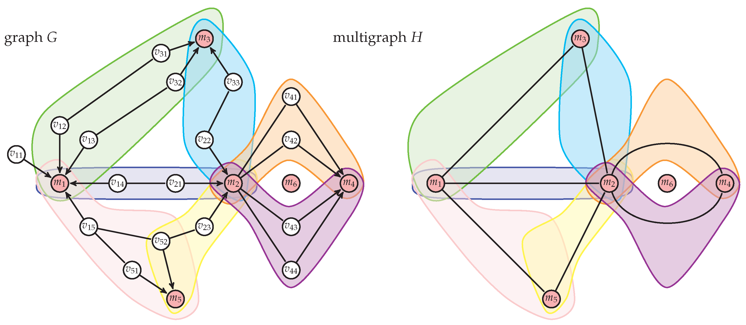
Figure 2 shows an example graph
G and the corresponding multigraph
H with marked bunches and edges. It is worth noting that special paths between vertices
and
were divided into two separate bunches due to vertex
lying inside the area between these paths. Moreover, it should be observed that there may exist vertices like
that do not belong to any bunch.
Lemma 4. The set consists of M–M special paths.
Proof. It is clear that each path has both endpoints in M and does not begin and end at the same vertex. Additionally, every internal vertex of P is in . Therefore, conditions (a) and (c) of Definition 2 are satisfied.
Now, assume for contradiction that condition (b) is not met. In this case, there must exist two paths
that intersect at some internal vertex
(see case “a” in
Figure 1). Since
, both paths
and
must end at the same vertex
, which contradicts the assumption that they cross. □
Definition 5. For a graph and any subset of vertices , we define the following operators:For simplicity of notation, instead of using the notation for a single vertex v, we will simply write , , etc. Definition 6. For a graph and a set of bunches , we define the subset of vertices T:The set T will be called the set of external vertices of bunches or, in short, the external vertices of bunches. Every vertex in that is not external is called an internal vertex of B. Definition 7. For a given bunch we define as the set of bunch vertices belonging to set T, i.e., . The set of remaining vertices excluding bunch endpoints is denoted as , i.e., .
Lemma 5. .
Proof. From Lemma 3, we know that the total number of bunches is at most for . Furthermore, each bunch has exactly two boundary paths, so in total we have at most boundary paths.
From the definition of special paths in bunches
, each boundary path can contain at most two vertices belonging to
. Since each vertex
by definition belongs to at least two different bunches, it is counted at least twice in our estimation. Therefore, we obtain the following:
which completes the proof. □
In the case of triangle-free graphs, we can obtain a better estimate for the number of vertices in the set T. This is due to the fact that triangle-free graphs have fewer edges compared to general planar graphs, which directly affects the structure of bunches.
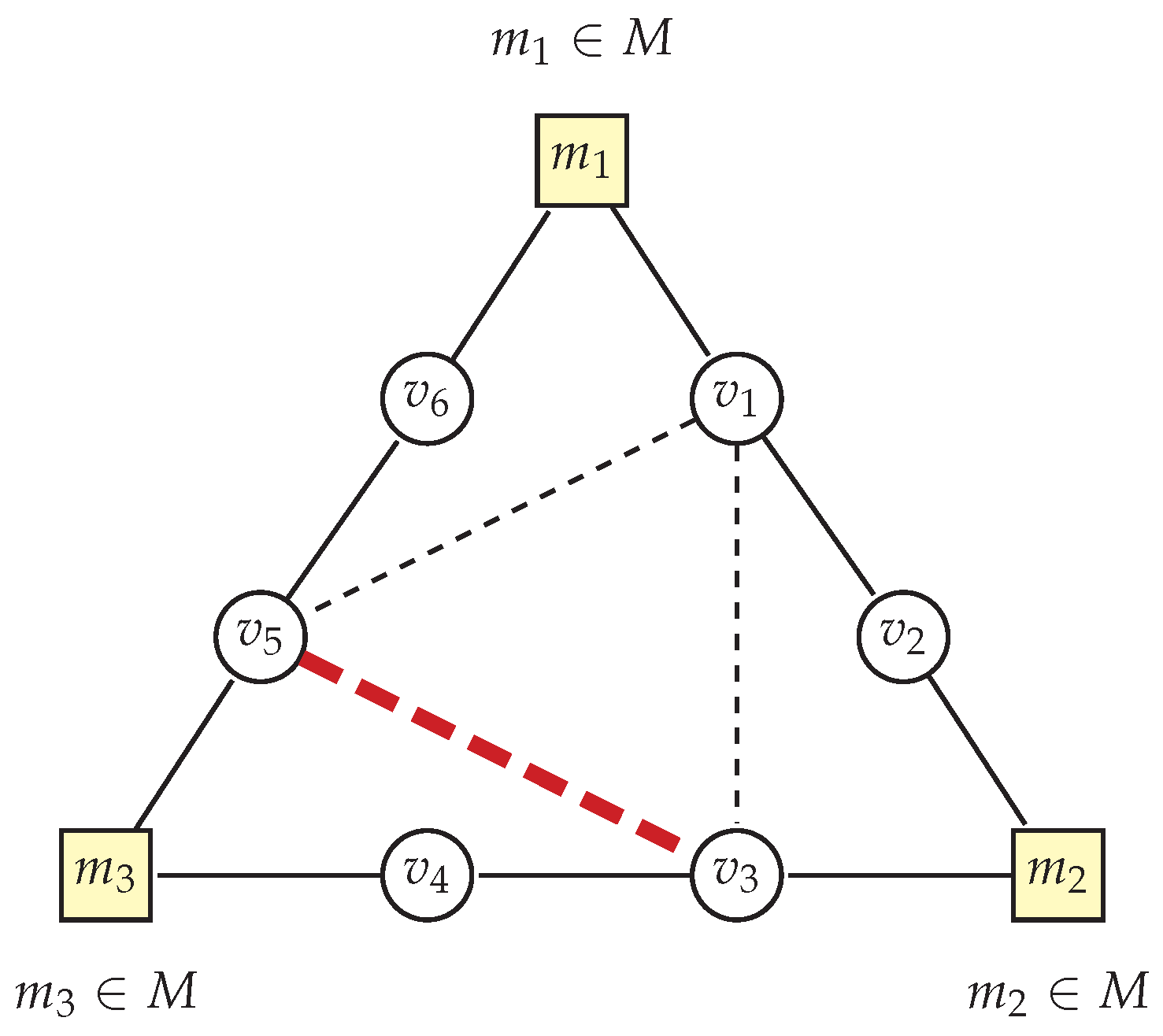
Lemma 6. For each face f of degree 3 in the bunch graph H of a triangle-free graph G, there are at most two vertices belonging to the set T that are incident to this face f.
Proof. Let us consider a face f of degree 3 in the bunch graph H. This face is bounded by three vertices belonging to the set M, which we denote as , , and . Each edge in graph H corresponds to a bunch in graph G, so we have three bunches associated with face f.
An example of such a degree 3 face is shown in
Figure 3, where vertices
,
, and
form a triangle, and between each pair of vertices from set
M there are two vertices not belonging to set
M:
Note that on each such path there can be at most two vertices from
by the definition of special paths in bunches
. Moreover, without loss of generality, let us assume that vertex
belongs to two bunches on this face. Vertex
belongs to the bunch with path
, so in order to belong to two bunches
must be connected to vertex
(the dashed line in
Figure 3 between
and
). Note that for such a situation to occur, vertex
must be outside face
f. For vertex
to belong to set
T that is incident to face
f, we must add edge
(also marked in
Figure 3 with a dashed line).
However, it is not possible for three vertices incident to a face of degree 3 to belong to
T. Otherwise, there would have to be three vertices from
lying on this face and they would have to be connected to each other. This is impossible in a triangle-free graph. This example is shown in
Figure 3. The potential edge between vertices
and
is marked in red with a bold dashed line. However, such an edge cannot exist in a triangle-free graph, as it would form a triangle with the existing edges (specifically with edges
and
). Consequently, vertex
lies only on one bunch (between
and
), and it does not belong to the bunch between
and
, because the path
would have five vertices, which exceeds the maximum path length in a bunch, which is four vertices.
From the analysis of possible connections of the vertices in a face of degree 3 in a triangle-free graph, it follows that we can have at most two vertices belonging to T that are incident to face f. In the presented example, these are vertices and .
Therefore, the maximum number of vertices belonging to T that are incident to a face f of degree 3 is two. □
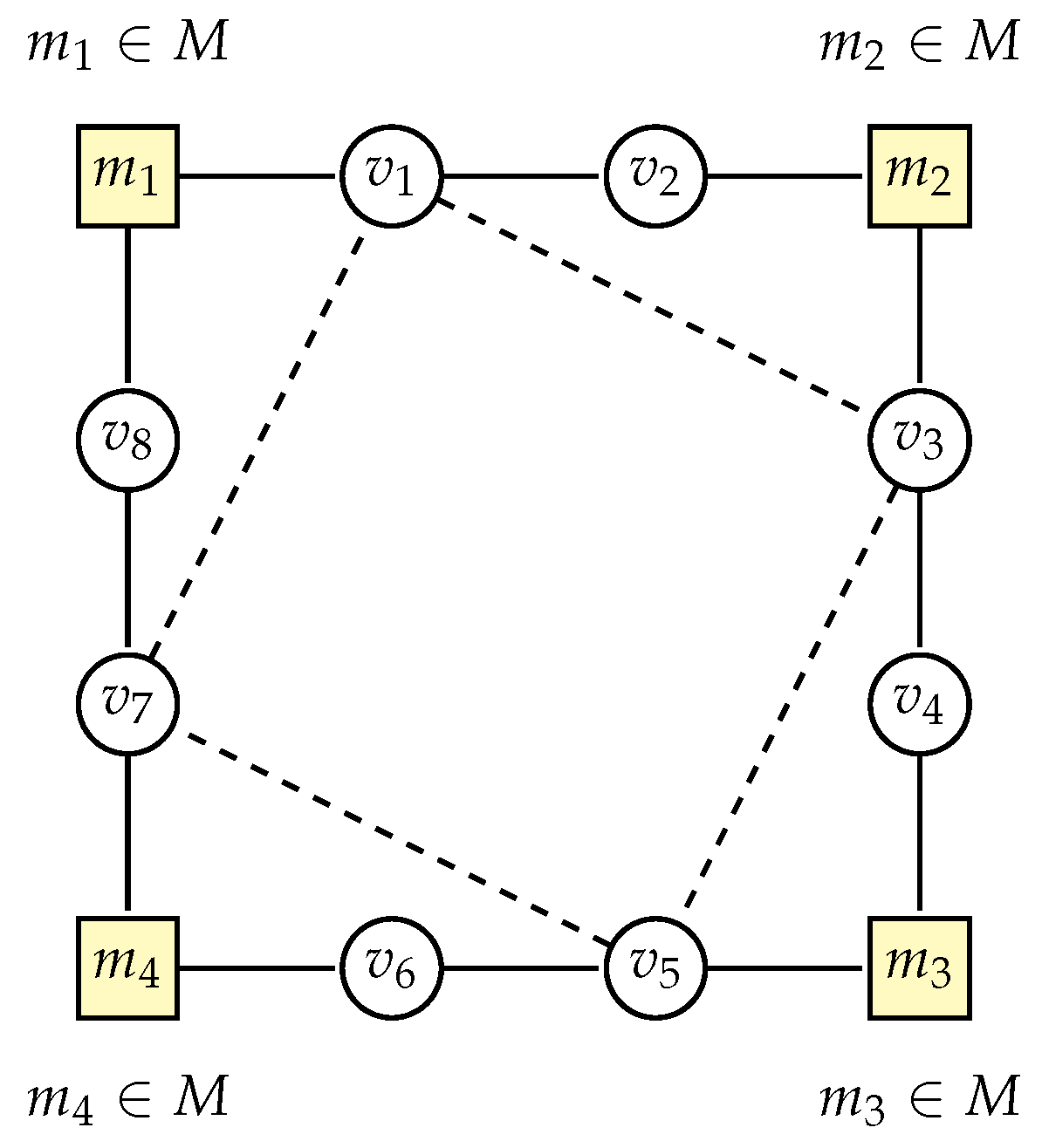
Lemma 7. For each face f of degree in the bunch graph H of a triangle-free graph G, the number of vertices belonging to the set T that are incident to this face f does not exceed the degree of the face, i.e., .
Proof. Let us consider a face f of degree in the bunch graph H. This face is bounded by vertices belonging to the set M. Each edge in graph H corresponds to a bunch in graph G, so we have bunches associated with face f.
Figure 4 shows an example of a face of degree 4, where vertices
,
,
, and
form a square, and between each pair of vertices from set
M there are at most two vertices from
:
Note that an edge such as
cannot exist in
Figure 4, because it would cause the considered face
f to have a degree less than the fixed value
k in graph
H.
Again, to obtain the maximum number of vertices belonging to
T that are incident to face
f, we must add dashed edges between “opposite” vertices, as shown in
Figure 4. However, there is an important difference compared to the case of a face of degree 3. In the case of a face of degree 3, we have only two vertices belonging to
T that are incident to face
f, while in the case of a face of degree
k we have
k vertices belonging to
T that are incident to face
f. Closing the “cycle” does not create a triangle in graph
G in this case.
Therefore, the maximum number of vertices belonging to T that are incident to a face of degree is . □
Lemma 8. For triangle-free graphs, .
Proof. We want to count the maximum number of possible vertices T in relation to the number of bunches, which is . Let us consider the bunch graph .
From Lemma 6, we know that for each face f in graph H with degree , there are at most two vertices belonging to T. Moreover, from Lemma 7, we know that for each face f in graph H with degree there are at most vertices . Let us note that each face with degree uses edges. We add the factor because it represents the number of missing edges needed to achieve the maximum number of edges in a face in graph H. Additionally, we multiply by 2 because each edge is adjacent to two faces, or to the same face twice. If we have a face with a higher degree, the number of bundles automatically decreases and, consequently, the number of edges in graph H decreases as well.
Hence, we can obtain the maximum ratio of the number of vertices
to the number of used edges in a face with degree
:
For
, we obtain
For
, we obtain
For
, the ratio will be even smaller. Therefore, the maximum ratio of the number of vertices
to the number of used edges is
and is achieved for faces with degree less than or equal to 4.
It should be noted that each edge (bundle) belongs to two faces, so the maximum number of vertices
is
From the proof in paper [
29], we know that the number of edges is bounded by
Substituting this estimate, we obtain
□
This improved estimation will be crucial for obtaining an approximation factor of 6 for the minimum dominating set problem in triangle-free graphs.
4. Definitions and Basic Properties
Before we proceed to estimate the approximation ratio for the dominating set returned by the algorithm, we need to introduce additional definitions.
First, we will introduce a mapping between vertices selected by the algorithm and vertices of the optimal dominating set. This mapping will allow us to relate the vertices chosen by the algorithm, which will enable us to effectively bound the number of selected vertices and prove a more accurate approximation ratio.
Definition 8. Let Γ
be the set of vertices selected by the algorithm, consisting of two subsets:Note that may contain vertices that are not added to the set , as some vertices might be replaced by during the second phase of the algorithm. —the set of vertices selected in the second phase of the algorithm and not added to .
—the set of vertices selected in the second phase of the algorithm and added to .
Finally, —the set of all vertices selected by the algorithm (not necessarily added to ).
Now we are ready to define the alpha function that will help us estimate the number of vertices added to the dominating set D.
This function will map the vertices selected by our algorithm to the vertices in the optimal dominating set, allowing us to establish a relationship between our solution and the optimal one.
Definition 9. Let be a function that assigns to vertices from Γ (selected as in phases 1 and 2 of the algorithm) a vertex . The function α is defined by the following cases:
- (a)
, where then .
- (b)
, where then .
- (c)
, where then .
Case 2: When a vertex , such that (from the definition of bunches), adds to the set D a vertex, as follows:
- (a)
, where then .
- (b)
, where then .
- (c)
, where then .
For all other cases, .
In summary, the function works as follows: if a vertex adds a vertex u to the set D then . Similarly, when a vertex adds a vertex u to the set D then , where is the vertex from M associated with v in the bunch definition.
The function plays a crucial role in the analysis of the algorithm by mapping the vertices selected by the algorithm to the vertices of the optimal dominating set M. This allows us to track which vertices from M are “responsible” for the vertices chosen by the algorithm. Through this mapping, we can precisely determine how many vertices the algorithm selects relative to the optimal solution, which is essential for proving the approximation ratio. The function accounts for both direct vertex selections and cases where the algorithm performs optimization by replacing one vertex with another (cases where vertex is added to set instead of ).
Definition 10. For each we also define counting functions: The function counts some internal vertices in bunches that are added to D. More precisely, includes the number of vertices added to lying inside a bunch and for which m is responsible. Additionally, it counts the vertices added to in phase 2 of the algorithm, for which vertex m is also responsible. The function also accounts for the vertices added in phase 2 as vertices instead of vertices (where vertex was selected by a vertex v, for which ). Furthermore, we also count vertex m itself if it belongs to the set .
Definition 11. We divide the set M into two disjoint subsets:
5. Lemmas and Proofs
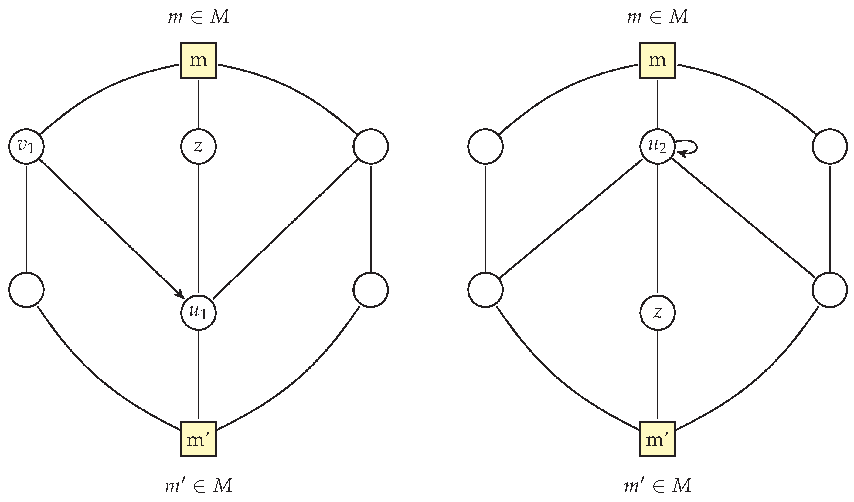
Lemma 9. Let G be a triangle-free graph and be an m–-bunch. If there exists a vertex adjacent to m such that then there exists a vertex such that within the same bunch B and u is adjacent to .
Proof. Consider an m–-bunch B and a vertex such that . Since , we know that and, thus, it is adjacent to either m or . Without loss of generality, we can assume that v is connected to m.
Since , there exist three different vertices in addition to m. First, note that cannot be connected to m (as they would form a triangle with v). Also note that due to the absence of triangles in graph G. Therefore, must be connected to . Since , all neighbors of vertex v belong to bunch B.
Let us number vertices so that is “between” and in the sense of the bunch structure. Then, it is easy to see that vertex is a neighbor of v and but cannot be connected to either or (as it would form a triangle). Therefore, must have degree 2, which completes the proof. □
Figure 5 illustrates the existence of a vertex of degree 2 in a bunch when there is a vertex of degree of at least 4. The left side shows a vertex
with a degree of at least 4 adjacent to
m, while the right side demonstrates how this implies the existence of a vertex
z with a degree of exactly 2 adjacent to
:
Lemma 10. Let B be an m–-bunch where the endpoint m has a degree at least 3 (). If m selects a vertex as then will be added to the set in phase 1 of the algorithm.
Proof. Let us assume by contradiction that the lemma’s assumptions are satisfied, but . From our assumption, we know that m has a degree of at least 4 (). Furthermore, from Lemma 9, we know that in bunch B there exists a vertex such that and u is adjacent to . Moreover, u is adjacent to a vertex v such that . According to the definition of phase 1 of the algorithm, vertex u with degree 2 selects vertex with the smallest ID among vertices with the highest degree in its closed neighborhood .
Since from our contradiction assumption we know that , vertex u cannot select vertex as , and, thus, will not be added to . Otherwise, m would be dominated and would not select any vertex as in phase 2 of the algorithm. We obtain a contradiction with the lemma’s assumption, which completes the proof. □
Lemma 11. Let be a vertex that is not dominated in the first phase of the algorithm, and let be the vertex chosen by v in step 12 of the algorithm instead of vertex . Then, .
Proof. Let us assume, by contradiction, that and vertex v chose instead of in phase 2 of the algorithm. First, note that cannot belong to , because vertex v adjacent to would not be considered in the second phase of the algorithm. Therefore, from our contradiction assumption that and the fact that we conclude that . Moreover, vertex was added to set instead of , which means the following:
- (1)
dominates a larger (in terms of inclusion) set of vertices not dominated by than , or
- (2)
dominates the same set of vertices not dominated by as , but has a smaller identifier than .
Since v added vertex to set instead of , we find that must have been added to set by another vertex, , in the second phase of the algorithm. However, note that since vertex v chose instead of in phase 2 of the algorithm, it follows from satisfying conditions (1) or (2) that vertex u would also choose instead of . We obtain a contradiction. Therefore, . □
Lemma 12. Let be such that . Then, .
Proof. Let us assume, by contradiction, that and the assumptions of the lemma are satisfied. Then, by the definition of the counting function , there exist at least two vertices chosen by neighbors of vertex m; let us denote them as .
Since , we have . First, let us assume that and belongs to some bunch B with endpoints m and . Then, is adjacent to m. Therefore, from Lemma 9, we know that there exists a vertex such that and z is adjacent to .
Since vertex z in phase 1 of the algorithm adds either or to set , vertex is dominated and, thus, cannot choose vertex as . We obtain a contradiction.
Therefore, we have . Similarly, there must exist a vertex z of degree 2, but in this time it is adjacent to . Then, vertex z in the first phase of the algorithm chooses vertex or as . However, since chose itself in phase 2 of the algorithm, we find that . Note that all neighbors of vertex are dominated. Thus, according to Lemma 10, we find that either or . Hence, we find that . □
Lemma 13. For a triangle-free graph, the number of external vertices selected by the algorithm is bounded by Proof. From Lemma 8, we know that for triangle-free graphs,
. Since the external vertices selected by the algorithm are a subset of all the external vertices, we have
□
7. Conclusions and Future Work
Our approximation ratio of 6 for the minimum dominating set problem in triangle-free graphs represents a significant improvement compared to previous results in the distributed setting. It is important to note that while sequential algorithms can achieve better approximation factors (as low as 5), our 6-approximation algorithm is the current best for distributed algorithms in the LOCAL model. Our analysis of the structure of triangle-free graphs allowed for a more precise estimation of the number of external vertices, which was crucial for achieving a better approximation ratio. Our approach is worth comparing with the recent work by Heydt et al. [
27], who reached an approximation ratio of
for triangle-free planar graphs.
Their algorithm works in three steps: first, they pick vertices that are “hard to cover” (meaning vertices whose neighborhood together with themselves cannot be dominated by a small number of vertices, e.g., two). Next, they build special sequences of vertices that cover many others, and, finally, they use linear programming to cover any remaining vertices. It is important to note that their method is a general algorithm that can be applied to any planar graph with an approximation ratio of , not just triangle-free graphs. Our algorithm takes a different approach to selecting vertices. We use the special bunch structure of triangle-free planar graphs rather than their more general method. This approach helps us obtain a better approximation ratio (6 instead of ) while still running in constant time in the LOCAL model. Our algorithm is also easier to understand and implement because it directly selects vertices based on their degree, instead of using complex sequences and linear programming methods.
It is worth noting that the bunch technique can also be applied to improve the approximation ratio for planar graphs in general. Using this technique, we achieved an approximation ratio of 19, which improved upon the previous result of 52. However, since this result was worse than the 11-approximation achieved in the work of Heydt et al. [
27], it was not presented in detail in this paper. Perhaps with a more thorough analysis of the bunch structure and appropriate modifications to the algorithm, there is potential for further improvements. Further research in this direction may potentially lead to additional results.
An interesting aspect to investigate would be the computational complexity of the presented algorithm in various distributed computing models, particularly in the CONGEST model, where only O(log n) bits can be exchanged in one round between vertices. It would be interesting to question whether using so-called short messages can achieve the identical approximation ratio.
In summary, the presented technique constitutes a promising step toward more efficient algorithms for the minimum dominating set problem in graphs with special structure and could serve as a starting point for further research in this field.


