Parallel CUDA-Based Optimization of the Intersection Calculation Process in the Greiner–Hormann Algorithm

Abstract

The Greiner–Hormann algorithm is a commonly used polygon overlay analysis algorithm. It uses a double-linked list structure to store vertex data, and its intersection calculation step has a significant effect on the overall operating efficiency of the algorithm. To address the time-consuming intersection calculation process in the Greiner–Hormann algorithm, this paper presents two kernel functions that implement a GPU parallel improvement algorithm based on CUDA multi-threading. This method allocates a thread to each edge of the subject polygon, determines in parallel whether it intersects with each edge of the clipping polygon, transfers the number of intersection points back to the CPU for calculation, and opens up corresponding storage space on the GPU side on the basis of the total number of intersection points; then, information such as intersection coordinates is calculated in parallel. In addition, experiments are conducted on the data of eight polygons with different complexities, and the optimal thread mode, running time, and speedup ratio of the parallel algorithm are statistically analyzed. The experimental results show that when a single CUDA thread block contains 64 threads or 128 threads, the parallel transformation step of the Greiner–Hormann algorithm has the highest computational efficiency. When the complexity of the subject polygon exceeds 53,000, the parallel improvement algorithm can obtain a speedup ratio of approximately three times that of the serial algorithm. This shows that the design method in this paper can effectively improve the operating efficiency of the polygon overlay analysis algorithm in the current large-scale data context.

1. Introduction

With the rapid development of Earth observations and geographic information perception tools, the ability to obtain spatiotemporal information has increased and the scale of spatial data has shown explosive growth [1,2,3]. Overlay analysis is a commonly used spatial analysis function in geographic information systems [4] and is an important and difficult issue in geographic data processing [5,6]. Common parallel methods include multicore parallelism, cluster parallelism, and GPU parallelism [7,8]. It is easy to transform multicore parallel algorithms, but this can achieve only small-scale parallelism; cluster parallelism has stronger parallel capabilities, but the transformation cost is large. GPUs contain thousands of computing cores and have natural parallel characteristics [9]. Therefore, GPU parallelism can achieve significant efficiency improvements with lower consumption costs. CUDA is a general-purpose parallel computing platform and programming model [10] that allows developers to use NVIDIA GPUs for high-performance computing. CUDA-based GPU parallelism has gradually become the mainstream strategy for optimizing polygon overlay analysis algorithms.

There are many excellent polygon overlay analysis algorithms in the current geographic information system field, which have different characteristics and are suitable for different polygons. The Liang–Barsky algorithm [11], Wang algorithm [12], Foley algorithm [13], Maillot algorithm [14], etc., can clip only arc polygons. The Cyrus–Beck algorithm [15], Andreev algorithm [16], etc., can clip only convex polygons. The Sutherland–Hodgeman algorithm [17] is more applicable than the aforementioned algorithms and can perform clipping operations for arbitrary polygons and convex polygons. This algorithm sets a clipping window and uses an edge of the window and its extension line to divide the plane into two parts: the visible side and the invisible side. By traversing the edge of each input polygon, the relative position relationship between the current edge and the clipping edge is determined. After each clipping is completed, a vertex sequence is output as the input for the next clipping step, and, finally, the clipping of the polygon is completed. The Weiler–Atherton algorithm [18] can handle clipping between arbitrary polygons, but it is prone to failure when dealing with overlapping edges. The algorithm traverses each edge of the input polygon to determine whether it intersects with the boundary of the clipping polygon, generates new boundary points on the basis of the intersection points, and thus draws the resulting polygon. The Martinez algorithm [19] can clip any polygon and is considered an extension of the plane scanline algorithm. The basic idea is to subdivide the border at the intersection points on the polygon boundary, determine the resulting boundary on the basis of whether the current boundary is inside another polygon, and connect the selected boundaries to form the final polygon. The main advantage of this algorithm is its high efficiency in terms of time complexity, but its steps are relatively complex, and it is not widely used. The Vatti algorithm [20] and the Greiner–Hormann algorithm [21] are recognized algorithms that can clip arbitrary polygons in a limited time and obtain correct results [22]. The Greiner–Hormann algorithm uses a bilinear linked list data structure and has a lower algorithmic complexity than the Vatti algorithm [23]. The clipping process is the same between the different operators, and only the resulting polygon outputs are different. Therefore, the Greiner–Hormann algorithm intersection operator is selected here for parallel GPU optimization.

As the scale of geospatial data continues to expand, polygon overlay analysis algorithms are becoming both more computationally intensive and more data intensive [24,25]. Research on the parallel optimization of polygon overlay analysis algorithms has important practical significance for improving algorithm efficiency and perfecting GIS theory. At present, many scholars have carried out parallel optimization of polygon overlay analysis algorithms and achieved a degree of acceleration. Mallika et al. [26] demonstrated a practical polygon clipping method based on line segment trees, which parallelized the algorithm via OpenMP instruction. Wu Liang et al. [27] designed and implemented a practical distributed spatial analysis framework, which effectively improved the efficiency of parallel spatial analysis calculations for processing massive spatial data in a distributed environment. Zhou Yuke et al. [28] proposed a parallel spatial analysis framework that combines MySQL and MPI to perform parallel storage and processing analysis of vector data. Qiu Qiang et al. [29] used the MPI programming model in a Linux cluster environment and adopted the average striping method to perform point inclusion test operations. Shi et al. [6] parallelized the intersection, union, difference, and XOR processing of overlay analysis in a multicore environment. They first filtered the clipping polygon and the clipped polygon using the minimum enclosing rectangle to exclude nonintersecting polygons. Zhang [30] classified and described in detail the characteristics of complex polygonal objects composed of single rings, multiple rings, and a large amount of node data under simple feature models, paying particular attention to how these objects form a multilink structure. On this basis, a set of polygonal object screening methods and parallel computing strategies based on multiple data bounding boxes were proposed and established. Zhao Sisi et al. [31] divided overlay analysis into two stages, namely, MBR filtering and polygon clipping, and applied a GPU. They improved the Weiler–Atherton algorithm by using a new intersection insertion method and a simplified algorithm for marking entry and exit points, combined with a parallel preprocessing algorithm, and proposed a GPU-based polygon clipping algorithm. Current research on parallelization methods for polygon overlay analysis algorithms has achieved certain results, but the calculation process in traditional polygon overlay analysis algorithms is tightly coupled with the data structure, making it difficult to achieve fine-grained parallelization [32,33]. Puri et al. [34] conducted fine-grained GPU parallelization on the Greiner–Hormann algorithm based on CUDA, but they only used the number of polygon vertices to measure the complexity of the data, and the experimental data were relatively small, and the thread modes were not diverse enough. The parallel algorithm in this paper effectively avoids its defects during optimization.

To address the above problems, this paper improves the most time-consuming intersection calculation step in the Greiner–Hormann algorithm by using multithreaded parallelism in CUDA and presents two kernel functions that implement an improvement algorithm based on GPU parallelization. Specifically, we first analyze the steps of the Greiner–Hormann algorithm, study its data structure and algorithm flow, and find the time-consuming parts that can run independently. Second, we perform fine-grained parallel transformation of the algorithm on the basis of the CUDA programming model. The intersection calculation and insertion process, which consumes the most time in the algorithm, is optimized via CUDA multithreading. The first kernel function assigns a thread to each edge of the subject polygon to perform intersection judgment with the clipping polygon, stores the number of intersection points in a variable and returns it to the CPU. The CPU allocates corresponding memory for the intersection points and then returns the memory to the GPU; the GPU then executes the second kernel function, calculates the coordinates of the intersection points and other information in parallel, and, finally, returns this information to the CPU. Finally, we select eight subject polygons with different shape complexities to execute the serial and parallel algorithms and use different thread combination modes to analyze the best thread mode of the algorithm after parallel transformation. Moreover, on the basis of the best thread mode, we statistically analyze the running time and speedup ratio of the serial and parallel algorithms to verify the improvement in the computational efficiency achieved by the parallel algorithm proposed in this paper. The research results show that the computational efficiency of the polygon overlay analysis algorithm is greatly improved through the parallel transformation of the Greiner–Hormann algorithm, which provides a method for performing spatial analysis of complex spatial geographic data.

2. Experimental Environment and Data

2.1. Experimental Environment

The experimental environment of this paper is described in

Table 1. Experimental environment.

CPU	Memory/GB	External Memory/TB	GPU	Development Tools
AMD Ryzen 9 5950X 3.4 GHz 16 core	128	4.5	NVIDIA GeForce RTX 3090	Visual Studio 2019

. The developed algorithm uses the C++ language.

2.2. Experimental Data

In this study, Chinese land use patch data were selected as the experimental data. The data were downloaded from OpenStreetMap (https://www.openstreetmap.org/, accessed on 1 July 2023). The data contain a variety of polygons, including simple polygons, concave polygons, polygons with holes, and self-intersecting polygons. These data have the general characteristics and application value of surface geographic data in overlay analysis. Moreover, to verify the feasibility of the method proposed in this paper, eight subject polygons of different shape complexities and one clipping polygon in the Chinese land use patch data were selected for overlay analysis. The experimental data are shown in Figure 1.

3. Methods

3.1. Calculation of Polygon Shape Complexity

Previous scholars have used the number of vertices to represent the complexity of polygons, but this method cannot accurately measure the complexity of polygons and cannot represent the relationship between shape complexity and algorithm operation efficiency. To calculate the shape complexity of the subject polygon and the clipping polygon, on the basis of Reference [35], this paper selects 6 polygon shape indicators to calculate the shape complexity of the subject polygon and the clipping polygon. The selected indicators are as follows: number of vertices (NOV), amplitude of the vibration (Ampl), number of holes (NOH), average nearest neighbor (ANN), concavity (Conv), and equivalent rectangular index (ER).

NOV refers to the number of all vertices on the boundary of the polygon. The more vertices a polygon has, the more complex it becomes. Ampl refers to the difference in perimeter between the vector polygon and its convex hull, which can measure the irregularity of the vector polygon. NOH refers to the number of inner rings of the polygon, which is also an important indicator used to measure the complexity of the polygon. ANN refers to the shortest distance between the current vertex and the remaining vertices, which can measure the degree of spatial clustering of vertices. Conv is the area difference between a vector polygon and its convex hull, which can reflect the degree of concavity inside the polygon. ER refers to the perimeter difference between a vector polygon and a rectangle with the same area. More complex polygons often have larger perimeter differences. The formulas for calculating the six polygon shape indices are shown in

Table 2. Polygon shape indices. ($A_{ch}$: area of the convex hull of the polygon; $A_{pol}$: area of the polygon; $A_{mbr}$: area of the minimum bounding rectangle of the polygon; $H_{hole}$: the number of holes in the polygon; $d_i$: the actual distance from the i-th point to its nearest neighbor; $P_{pol}$: perimeter of the polygon; $P_{ch}$: perimeter of the convex hull of the polygon; $P_{mbr}$ perimeter of the minimum bounding rectangle of the polygon; $P_{ear}$ perimeter of an equal-area rectangle of the polygon).

Polygon Shape Index	Formula
Number of vertices (NOV)	$NOV=V_{pol}$
Amplitude of the vibration (Ampl)	$Ampl=(P_{pol}-P_{ch})/P_{pol}$
Number of holes (NOH)	$NOH=H_{hole}$
Average nearest neighbor (ANN)	$ANN={\displaystyle \frac{{\displaystyle \sum _{i=1}^n{d}_i}}{n}}/{\displaystyle \frac{0.5}{\sqrt{n}/A_{pol}}}$
Concavity (Conv)	$Conv=(A_{ch}-A_{pol})/A_{ch}$
Equivalent rectangular index (ER)	$ER=P_{ear}/P_{pol}=\sqrt{{\displaystyle \frac{A_{pol}}{A_{mbr}}}}\times {\displaystyle \frac{P_{mbr}}{P_{pol}}}$

.

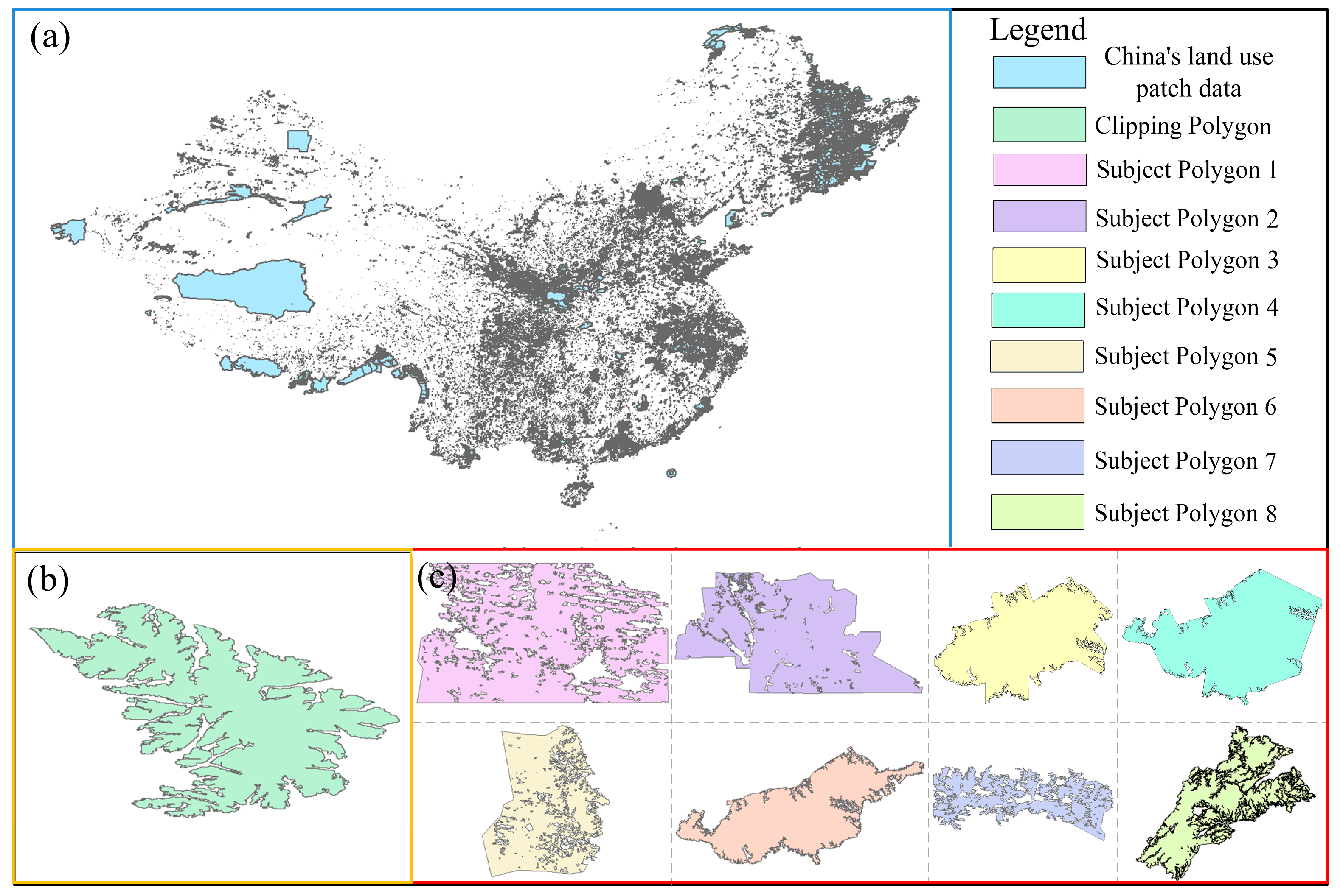
In this paper, 100,000 polygons are randomly selected as the subject polygons in the Chinese land use patch data, and the six index values of NOV, Ampl, NOH, ANN, Conv and ER of the target polygons are calculated as independent variables. A complex polygon is selected as the clipping polygon and overlaid with the 100,000 target polygons. The time of the overlay analysis is used as the dependent variable, and the algorithm selects the intersection operator of the Greiner-Hormann algorithm. Before the overlay analysis, the centroid of the subject polygon and the clipping polygon need to coincide to ensure the success of the overlay analysis. The selected indicators were diagnosed for collinearity using IBM SPSS Statistics 27 software to ensure that there was no correlation between the variables, and then a multivariate linear stepwise regression analysis was performed. After screening and analysis, the final six independent variable indicators were retained, and they were all closely related to the running time of the overlay analysis algorithm. The constructed shape complexity model is shown in Formula (1).

$$C=0.966x_1+0.041x_2+0.027x_3-0.019x_4+0.016x_5+0.011x_6,$$

(1)

where $C$ is the shape complexity of the intersection operator of the Greiner–Hormann algorithm, $x_1$ is NOV, $x_2$ is Ampl, $x_3$ is NOH, $x_4$ is ANN, $x_5$ is Conv, and $x_6$ is ER.

After the shape complexity model is constructed, the six indicators of the subject polygon and the clipping polygon are substituted into the constructed shape complexity model to obtain the shape complexity of the subject polygon and the clipping polygon. The vertices and complexity information of the eight subject polygons and the clipping polygon are shown in

Table 3. Experimental data.

Polygon Data	Number of Vertices	Polygon Shape Complexity
Subject Polygon 1	29,642	28,642
Subject Polygon 2	49,995	48,318
Subject Polygon 3	50,882	49,897
Subject Polygon 4	52,964	52,006
Subject Polygon 5	54,658	53,165
Subject Polygon 6	67,475	65,180
Subject Polygon 7	82,556	81,056
Subject Polygon 8	97,203	93,900
Clipping Polygon	28,768	27,352

.

3.2. Greiner–Hormann Algorithm

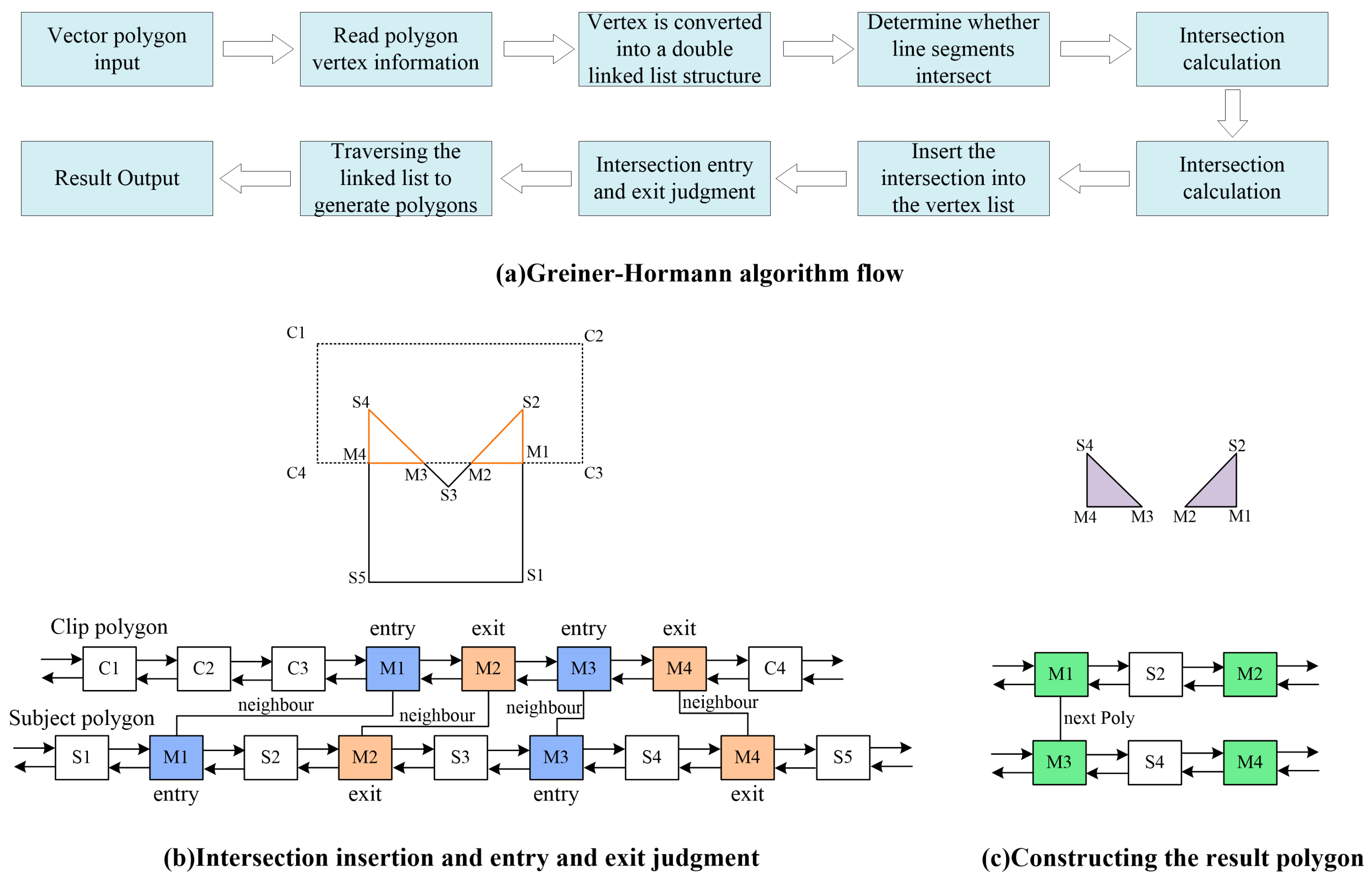
The Greiner–Hormann algorithm is a polygon clipping algorithm proposed by Greiner and Hormann in 1998. This algorithm treats the polygon clipping problem as the task of finding the partial boundary of one polygon from the interior of another. The main steps of the Greiner–Hormann algorithm are data reading and preprocessing, intersection calculation and insertion, intersection entry and exit judgment, and the resulting polygon output. The Greiner–Hormann algorithm flow chart is shown in Figure 2. The detailed steps of the algorithm are as follows.

(1) Data reading and preprocessing. The preprocessing stage of the Greiner-Hormann algorithm refers to the process of storing the vertex data of the subject polygon and the clipping polygon into different doubly linked lists.

(2) Intersection calculation and insertion. The core of the intersection calculation process is to determine the relationship between points and polygons and to find the intersection of line segments. The relationship between a point and a polygon is determined via a rotation number algorithm, which uses line segments to connect the point and all the vertices of the polygon, calculates the angles between all the points and the lines connecting adjacent vertices, and finally calculates the number of rotations on the basis of the accumulated angles, with every 360° sum being equivalent to one rotation. When the number of rotations is 0, the point is outside the closed curve. The cross-product method is used to determine whether the line segments intersect, and then the intersection of the line segments is calculated via vectors. Then, the intersection point is inserted into the subject polygon and clipping polygon linked list based on the calculated intersection point information.

(3) Entry and exit determination for the intersection point. The intersection point is marked as an entry point or an exit point on the basis of the calculated intersection information.

(4) Output of the resulting polygon. The polygon list is traversed after the intersection point is inserted, and the resulting polygon is output according to the algorithm operator.

3.3. Time Consumption Analysis of the Greiner–Horman Serial Algorithm

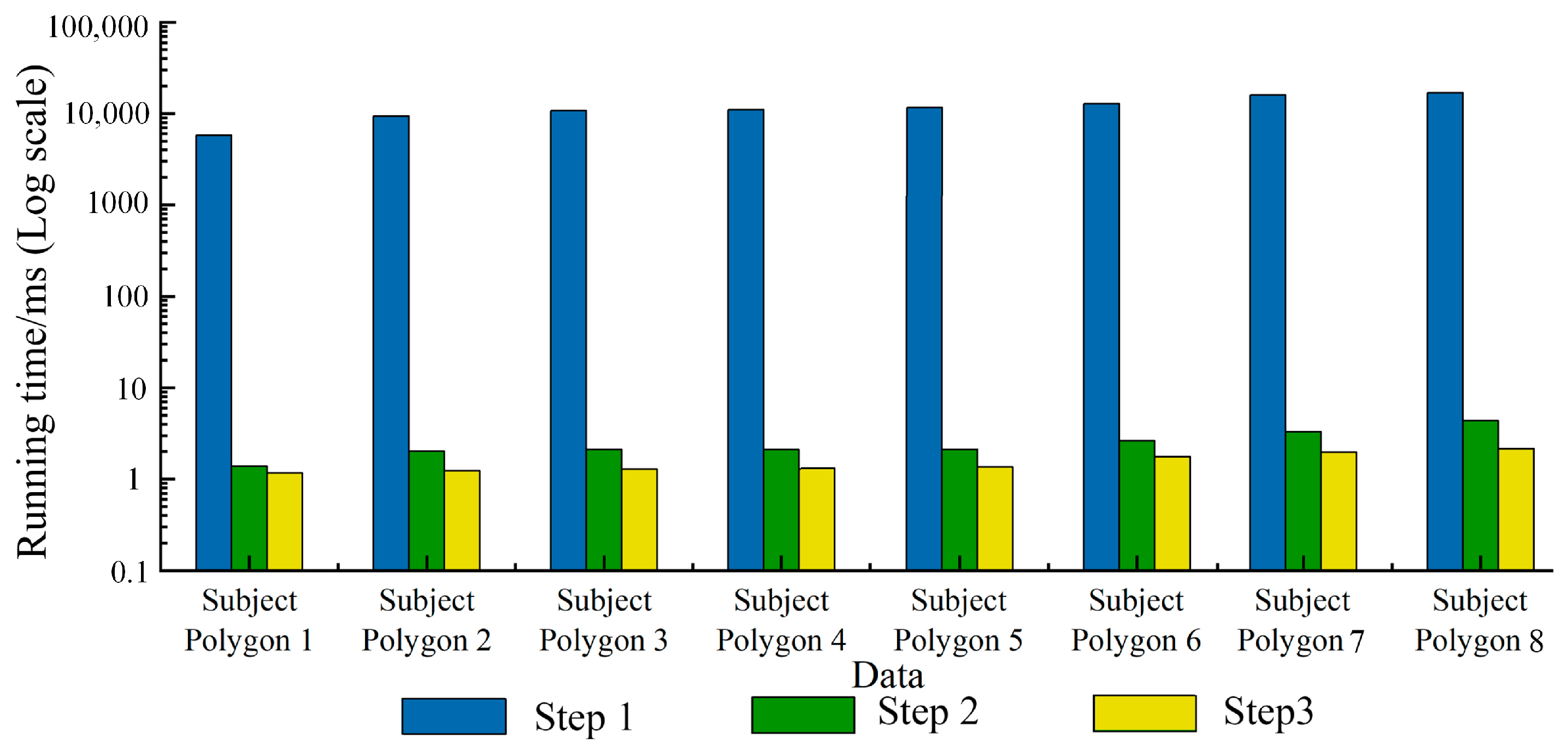
The core process of the Greiner–Hormann algorithm is divided into three steps. The first is to calculate the intersection of the line segments and insert them into the polygon list; the second is to determine and mark the entry and exit status of each intersection; finally, the list is traversed, and the resulting polygon is output according to the operator. This paper statistically analyzes the time consumption of each step of the intersection operator of the Greiner–Hormann algorithm. To avoid random effects, the eight complex polygons selected from the Chinese land use patch data mentioned above are used as the subject polygons and overlaid with the clipping polygon for analysis.

To ensure the effectiveness of clipping, the centroids of the eight subject polygons are firstly overlapped with the centroid of the clipping polygon. Then, the eight subject polygons are overlaid with the clipping polygon one by one. Finally, the time consumption of each step is determined. The time consumption values are shown in Figure 3. In the figure, step 1 is the calculation and insertion of the intersection points, step 2 is the determination of whether each intersection point is an entry or exit, and step 3 is the generation of the resulting polygon. As shown in Figure 3, the algorithm takes the most time in step 1, which can be thousands or even tens of thousands of times longer than step 2 and step 3. Steps 2 and 3 account for a small proportion of the overall running time of the algorithm—only a few thousandths of the total time—and have a low impact on the overall running time of the algorithm. There is no practical significance to optimizing these steps, so parallel optimization of these two steps is not considered. Step 1 accounts for more than 99% of the time of the entire algorithm, and it plays a decisive role in the running time of the intersection operator of the Greiner–Hormann algorithm. Therefore, optimizing the intersection calculation and insertion steps in the Greiner–Hormann algorithm is highly important for improving the efficiency of the algorithm.

3.4. Parallel Optimization Method for the Greiner–Hormann Algorithm

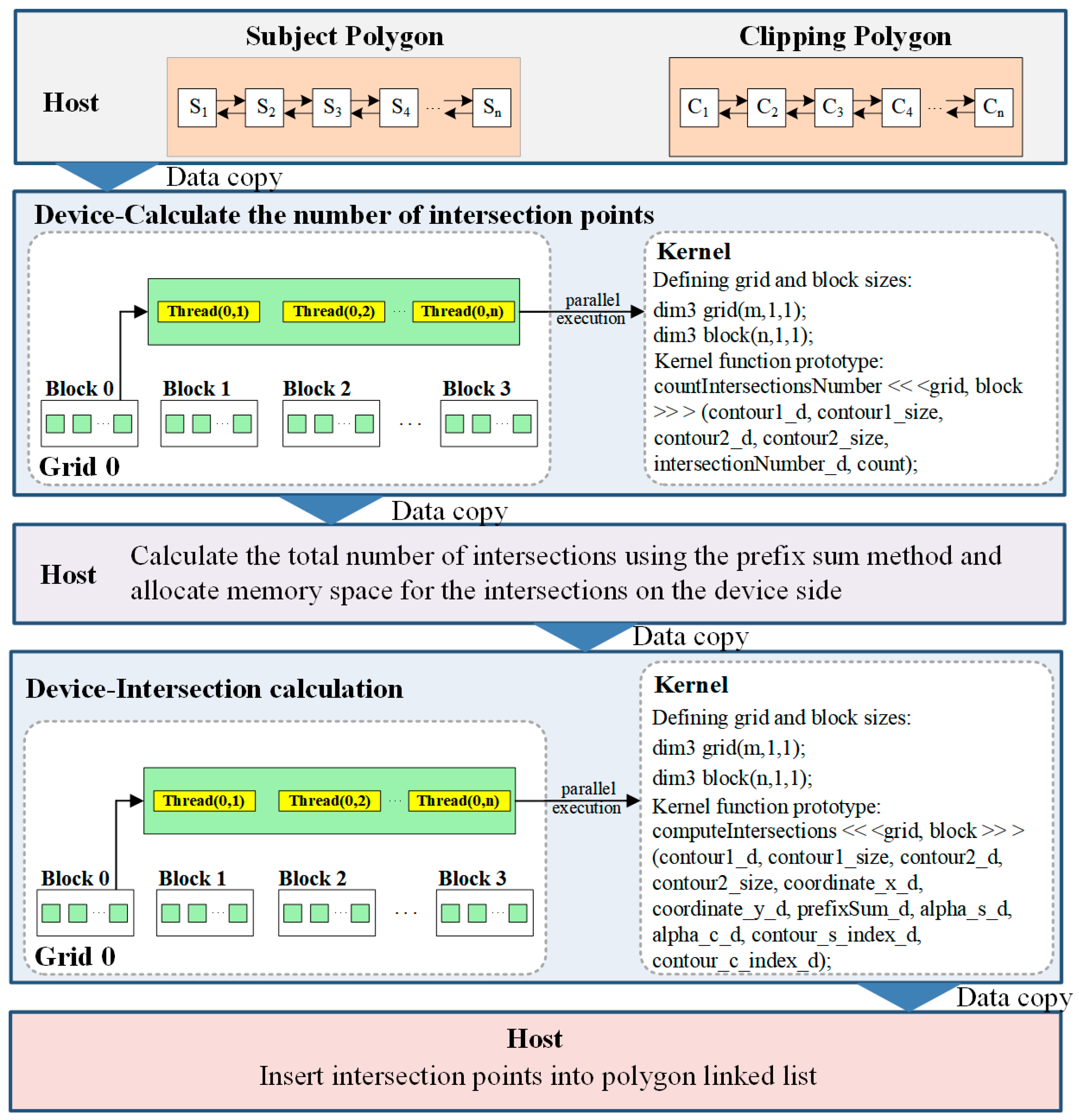
The detailed process of intersection calculation and insertion in the Greiner–Hormann algorithm involves intersecting each edge of the subject polygon with each edge of the clipping polygon, determining whether there is an intersection, and inserting the intersection into the bilinear linked list for the subject polygon and the clipping polygon. As seen from the previous section, this step takes the most time, and the processes of intersecting each line segment of the subject polygon are independent of each other, which makes this step suitable for parallel GPU optimization via CUDA.

In CUDA programming, the CPU is called the host, and the GPU is called the device. The host and the device execute different code tasks. The overall code operation of CUDA is divided into the CPU operation part and the GPU operation part. The CPU is responsible for logic control and for using and discarding memory and video memory, and the GPU is responsible for executing the kernel function, with which the parallel operations of CUDA are mainly carried out. The parallel GPU algorithmic optimization based on CUDA copies data from the host to the device, calls multiple threads to execute the kernel function, optimizes the independent time-consuming steps of the algorithm, and finally copies the calculated results from the device to the host.

This paper mainly writes kernel function to optimize the Greiner–Hormann algorithm for two parts: line segment intersection judgment and intersection point calculation. First, the double-linked list vertex data of the subject polygon and the clipping polygon are copied from the host to the device, and the first kernel function designed in this paper is executed to make intersection judgments. This function allocates a CUDA thread to each edge of the subject polygon to determine whether it intersects with each edge of the clipping polygon and stores the number of intersections in the variable count; second, the variable is transferred from the device back to the host, and the total number of intersections is calculated by the host via the prefix sum method. Then, storage space is allocated on the device according to the total number of intersections. The second kernel function intersection calculation designed in this paper is executed to calculate the coordinates of the intersection, the distance from the intersection to the two polygon edges, and the indices of the two edges that generate the intersection and store them in their respective arrays in order. Finally, all the calculated intersection data are transmitted back to the host. The intersection point is inserted into the double-linked list of the subject polygon and the clipping polygon according to the calculated intersection point information. The parallel CUDA optimization process for the Greiner–Hormann algorithm is shown in Figure 4.

4. Analysis of GPU Parallel Optimization Results

4.1. Analysis of the Parallel Optimization Efficiency of Different Thread Modes

Different subject polygons have different numbers of vertices and edges, which results in different total numbers of threads being called when executing parallel algorithms. The total number of threads called by each subject polygon is the same as its number of vertices, and the total number of threads is defined by the number of thread blocks and the number of threads contained in each thread block. Therefore, when calling multithreaded executions of parallel algorithms for each subject polygon, different thread combination modes can be used to test the optimization of the algorithm under different thread modes while ensuring that the total number of threads remains unchanged. For example, when the total number of threads is 128, two thread blocks are used, each of which has 64 threads, and four thread blocks are used, each of which has 32 threads. All 32 threads constitute a warp, which is the basic unit of parallel processing. Threads in a warp execute the same instructions at the same time, so the number of threads in each thread block is best set to a multiple of 32.

This paper conducts a statistical analysis on the running time of serial and parallel algorithms executed in different thread modes for eight subject polygons with different shape complexities. Six different thread modes are used in the parallel optimization process of each data point, namely 64, 128, 256, 512, 768, and 1024 threads per thread block. The running results are shown in Figure 5.

According to Figure 5, in a parallel environment, when a single thread block for subject polygons 1, 3, 7, and 8 contains 64 threads, the algorithm running time is the shortest; when a single thread block for subject polygons 2, 4, 5, and 6 contains 128 threads, the algorithm running time is the shortest. Regardless of the amount of data, the parallel algorithm runs fastest when two thread modes are used: a single thread block containing 64 threads and a single thread block containing 128 threads. When the number of threads is greater than 128, the algorithm execution time begins to gradually increase. This is because when there are too many threads, there are resource competition problems. When the number of called threads exceeds a certain limit, the excess threads will enter a waiting state, reducing the overall efficiency of the algorithm. As shown in Figure 5, when the Greiner–Hormann parallel algorithm is executed on data of different volumes, it may not achieve a higher running speed than the serial algorithm. Different data yield different performances; some can lead to speed improvements by several times, and some are several times slower than the serial algorithm.

4.2. Parallel Algorithm Acceleration Analysis

To intuitively study the optimization of GPU parallelization algorithms for data of different complexities, the thread mode with the best algorithm running efficiency is selected for the above eight subject polygon datasets and compared with the serial algorithm, and the running time and acceleration ratio of executing the parallel algorithm on different datasets are statistically analyzed. The speedup ratio refers to the ratio of the running time of the serial algorithm to that of the parallel algorithm, as shown in Formula (2):

$$S=T_1/T,$$

(2)

where $S$ is the acceleration ratio, $T_1$ is the running time of the serial algorithm, and $T$ is the total running time of the parallel algorithm.

Figure 6 shows the running time and speedup ratio of the serial and parallel algorithms for data of different complexities. When the complexity of the subject polygon is 28,642, 48,318, 49,897 and 52,006, the parallel improved Greiner–Hormann algorithm does not achieve a speed improvement. It is 2.9, 3.7, 3.7, and 3.6 times slower than the serial algorithm, respectively. The speedup ratios are 0.34, 0.27, 0.27, and 0.28, respectively, all of which are less than 1. However, when the polygon complexity is greater than or equal to 53,165, the parallel algorithm is significantly more efficient than the serial algorithm, achieving speedup ratios of 3.09, 2.68, 2.95, and 3.07 times. The acceleration effects for the four relatively large polygons are similar, and the speed increase is approximately three times. When the data complexity reaches a certain level, the Greiner–Hormann algorithm with the parallel improvement proposed in this paper can lead to an obvious acceleration improvement. That is, the acceleration effect can only be achieved when the total number of called threads reaches a certain number. When the number of threads is too small, data copying takes up more time, and the time saved by the parallel algorithm is not enough to compensate for the considerable time consumption caused by data copying, so the running speed of the algorithm cannot be improved. When the number of threads increases to a certain extent, the runtime reduction achieved by the parallel algorithm outweighs the additional time consumed by data copying, and the algorithm efficiency is improved accordingly. Therefore, when the subject polygon complexity is greater than 53,000, the method proposed in this paper can significantly reduce the runtime of the intersection operator of the Greiner–Hormann algorithm and improve the algorithm efficiency.

5. Discussion

Vector polygon overlay analysis is one of the basic functions of GIS spatial analysis. Its algorithm data structure is complex, and the calculations are difficult. Traditional serial algorithms are time-consuming, whereas parallel optimization by a GPU based on CUDA can effectively improve the calculation efficiency of vector polygon overlay analysis algorithms. The Greiner–Hormann algorithm is one of the most commonly used polygon overlay analysis algorithms. It uses a double-linked list structure to store vertex data. The intersection calculation step in the algorithm has a significant effect on the overall operation efficiency of the algorithm. Therefore, this paper uses the multithreaded parallelism of CUDA to improve the intersection calculation step, which is the most time-consuming step in the Greiner–Hormann algorithm. Two kernel functions are designed to implement a GPU parallel improvement algorithm based on CUDA multithreading. Additionally, eight subject polygons of different shape complexities and one clipping polygon are selected, and overlay analysis is performed on them via the serial algorithm and the method proposed in this paper. The results show that the computational efficiency of the polygon overlay analysis algorithm is improved by parallelizing the Greiner–Hormann algorithm, and a satisfactory acceleration ratio is achieved via the GPU hardware platform. This method is a valuable reference for improving the spatial analysis of complex spatial geographic data.

Although this paper improves the Greiner–Hormann algorithm through GPU parallelization on the basis of CUDA multithreading, it does not improve other polygon overlay analysis algorithms and does not apply other parallel architectures. In the future, we will conduct more in-depth research and analysis of the Greiner–Hormann algorithm, aim to find parts that are appropriate for parallel GPU improvement to increase the algorithm’s operating efficiency, and consider implementing parallel GPU transformation of other polygon overlay analysis algorithms on the basis of CUDA. Moreover, our future work will examine the hybrid parallelization of CPUs and GPUs to more effectively improve the efficiency of the polygon overlay analysis algorithm. Adjusting this method to solve computational geometry problems such as 3D polygon overlay is also our key research direction.

6. Conclusions

The parallel optimized polygon overlay analysis algorithm can significantly reduce the time cost of complex analysis tasks, provide technical support for efficient processing of large-scale data, and demonstrate its broad application potential in the fields of GIS and computer graphics. In the field of GIS, this method can efficiently handle operations such as spatial query and regional statistics; in the field of computer graphics, it can be used for complex polygon rendering, collision detection and dynamic scene simulation, significantly improving processing efficiency.

This paper uses CUDA multi-threaded parallelism to improve the intersection calculation process, which is the most time-consuming in the Greiner-Hormann algorithm, and implements a GPU parallel improved algorithm based on CUDA multithreading. Moreover, eight subject polygons with different shape complexities and one clipping polygon are selected, and overlay analysis operations are performed on them via the serial algorithm and the method proposed. The results are as follows.

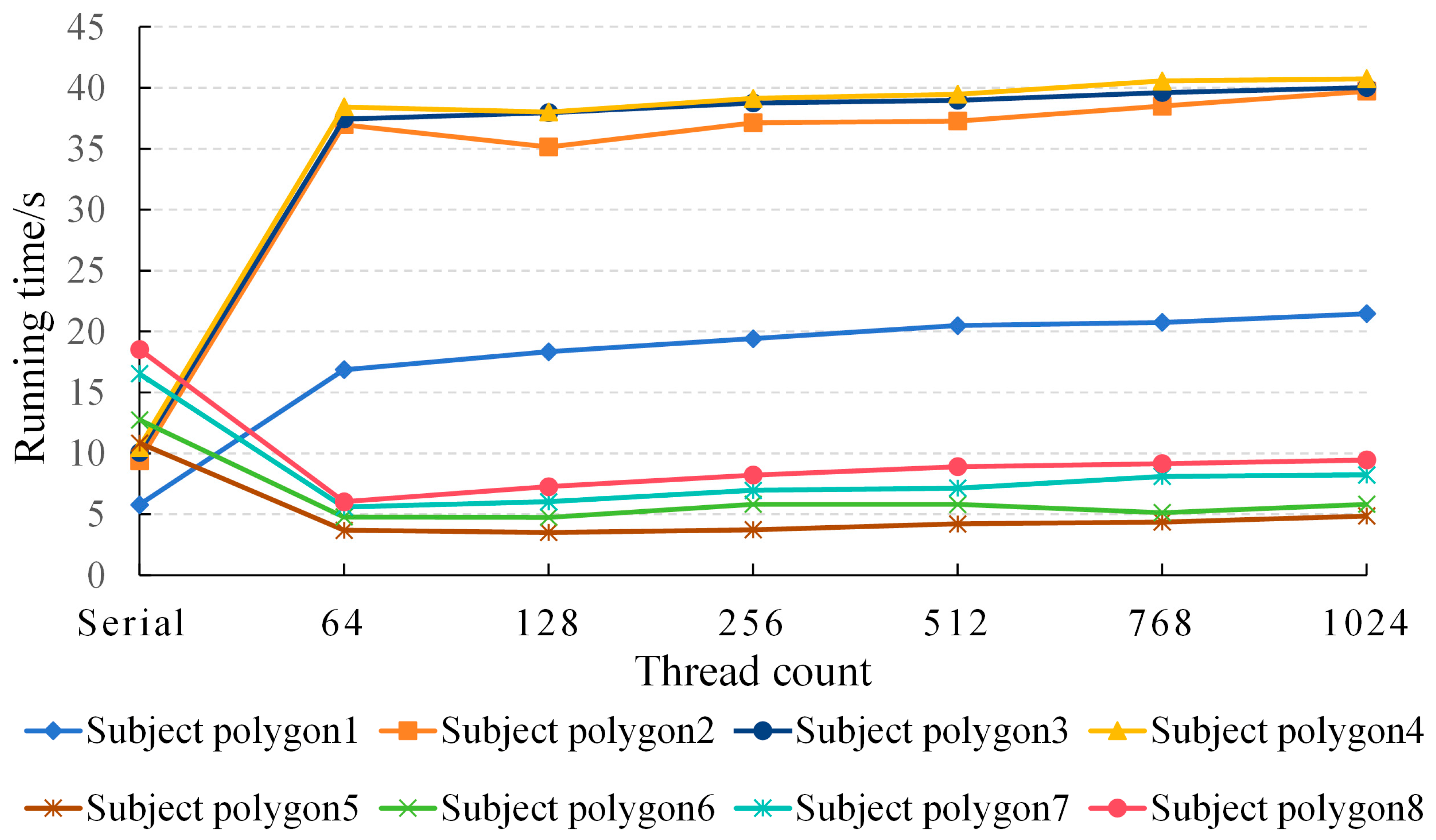
(1) The optimal thread mode for the parallel GPU improvement method proposed in this paper is when the number of threads in each CUDA thread block is 64 or 128, which can achieve the best parallel efficiency. This is because when there are too many threads in a single thread block, it will lead to resource competition and reduce computing efficiency.

(2) In the optimal thread mode, when the subject polygon shape complexity is greater than 53,000, the time saved by the parallel algorithm is significantly greater than the time spent on data copying, which significantly improves the efficiency compared with that of serial calculation, and a speedup ratio of approximately three can be achieved.

In summary, the method proposed in this paper increases the computational efficiency of the polygon overlay analysis algorithm through the parallel optimization of the Greiner–Hormann algorithm, and a new method and theoretical basis are provided for the spatial analysis of complex spatial geographic data.