Guided Particle Swarm Optimization for Feature Selection: Application to Cancer Genome Data

Abstract

Feature selection is a crucial step in the data preprocessing stage of machine learning. It involves selecting a subset of relevant features for use in model construction. Feature selection helps in improving model performance by reducing overfitting, enhancing generalization, and decreasing computational cost. Techniques for feature selection can be broadly classified into filter methods, wrapper methods, and embedded methods. This paper presents a feature selection method based on Particle Swarm Optimization (PSO). The proposed algorithm makes use of a guided particle scheme whereby three filter-based methods are incorporated. The proposed algorithm addresses the issue of premature convergence to global optima compared to other PSO feature-based methods. In addition, the algorithm is tested on very-high-dimensional genome data that include up to 44,909 features. Results of an experimental comparison with other state-of-the-art feature selection algorithms show that the proposed algorithm produces overall better results.

1. Introduction

Feature selection is a fundamental challenge in analyzing high-dimensional data, where datasets often contain numerous irrelevant or redundant features. Removing these features enhances predictive accuracy, reduces computational complexity, and improves model interpretability. By selecting the most relevant subset, models can focus on informative data, leading to more efficient and accurate predictions.

In bioinformatics, feature selection helps identify key biological markers or genes associated with specific processes or diseases, enabling deeper insights into biological mechanisms while improving predictive reliability. It is also widely applied in fields such as finance, healthcare, and text classification, where efficient handling of high-dimensional data is essential.

As a crucial step in data preprocessing, feature selection reduces overfitting, enhances generalization, and decreases computational costs. Methods for feature selection are typically categorized into filter, wrapper, and embedded approaches [1,2].

Filter-based feature selection methods utilize statistical measures in order to rank features or to give various features in a dataset a numerical rank in order to be able to discard irrelevant features with a low statistical score. Filter-based methods are often computationally efficient, but they sacrifice accuracy due to the fact that they look at the features individually without taking into account the relationships between features. For example, two features may be insignificant on their own, but when paired together, they might heavily affect the data.

Wrapper methods are often referred to as trial-and-error methods because they take into account every possible combination of features and choose the best one. As a result, wrapper methods for feature selection are often the most computationally expensive, but yield the most accurate results. The work being performed focuses on performing feature selection for highly dimensional data (large number of features), so wrapper-based approaches take an incredibly long time to run; thus, testing them has proven to be difficult.

Embedded methods perform feature selection during the model training process. The benefit of these methods is that they take into account interactions between features, something that filter-based approaches completely ignore. Embedded methods often provide a good balance between computational cost and accuracy.

A hybrid method can be any combination of two types of feature selection methods or even a feature selection method and another algorithm that may not generally be used for feature selection.

2. Related Work

Feature selection is a critical process in data mining and machine learning, aiming to identify the most relevant features from large datasets to improve model performance and reduce dimensionality. Nature-inspired algorithms have shown significant promise in optimizing feature selection [3]. This section expands on recent advancements and related work in this area.

A comprehensive study focused on the scalability of feature selection algorithms in the context of dynamic data generated by web-based applications and the Internet of Things (IoT) [4]. The research emphasized the limitations of existing dimensionality reduction techniques when dealing with noisy and rapidly inflating datasets. The study concluded that feature selection methods are essential for reducing data load and avoiding overfitting, thereby improving the efficiency of machine learning models.

Another comprehensive survey examined various nature-inspired metaheuristic methods for feature selection [5]. The study focused on the representation and search algorithms, highlighting their potential for global search and optimization. The survey provided an analysis of the advantages and disadvantages of different approaches, offering guidance for future research to address unresolved issues in the literature.

Looking at particular nature-inspired algorithms, the Genetic Algorithm (GA) is one of the most widely used algorithms for feature selection. GA mimics the process of natural selection by generating a population of candidate solutions and iteratively evolving them to find the optimal feature subset. A study applied GAs for feature selection in medical diagnosis, demonstrating significant improvements in classification accuracy and computational efficiency [6].

In [7], a feature selection method using the Ant Colony Optimization (ACO) algorithm, aiming to address the challenges posed by high-dimensional data. By employing a heuristic distance directly in the probability function, the algorithm avoids the need for subattribute sets and iteratively creates a frequency order list to determine feature importance. The technique’s effectiveness is validated through experiments that compare it with fifteen other algorithms, using identical datasets, classifiers, and performance metrics. The paper also demonstrates how feature selection improves classification performance and evaluates the convergence performance of the proposed method, highlighting its effectiveness in managing complex, multidimensional data.

In [8], a novel feature selection architecture integrating metaheuristic techniques with evolutionary algorithms and chaos theory is introduced. The proposed method leverages evolutionary concepts, such as mutation and crossover operators from Genetic Algorithms, to enhance search space exploration and exploitation. Additionally, a chaotic map function generates new random feature subsets to improve the optimization process. The method was tested on 10 datasets across various machine learning models, showing significant performance improvements compared to existing methods.

A feature selection architecture designed to enhance machine learning model performance by selecting relevant features and eliminating redundancy was introduced in [9]. The architecture combines metaheuristic techniques, evolutionary algorithms, and chaos theory to address high-dimensional data challenges. Key elements include Genetic-Algorithm-inspired mutation and crossover operators for efficient search and a chaotic map function for generating random feature subsets. Testing on 10 datasets demonstrated significant performance improvements compared to existing methods.

The study in [10] improved feature selection (FS) in hyperspectral image (HSI) classification by proposing a new filter–wrapper (F-W) framework to enhance swarm intelligence and evolutionary algorithms (SIEAs). The performance of ten SIEAs under this framework is evaluated using three HSIs, focusing on accuracy, selected bands, convergence rate, and runtime. Results show that overall, the SIEAs outperform traditional FS methods, achieving higher accuracy and efficiency, especially in complex scenes.

Particle Swarm Optimization (PSO) is also a popular evolutionary computation (EC) method that has been widely applied to feature selection problems. For example, an adaptive Particle Swarm Optimization (PSO) method for feature selection that overcomes the limitations of traditional PSO by incorporating adaptive parameter updating and leadership learning strategies is presented in [11]. Experimental results on 10 UCI datasets show that the proposed method outperforms other algorithms in both exploration and exploitation, selecting fewer than 8% of the original features while achieving more effective feature subsets than six traditional feature selection methods.

Binary Particle Swarm Optimization (BPSO) is a discrete variant of the Particle Swarm Optimization (PSO) algorithm, designed to handle optimization problems where variables are binary (i.e., they can take on values of 0 or 1). In traditional PSO, particles adjust their positions and velocities in a continuous search space to find optimal solutions. However, BPSO modifies this approach to operate within a binary search space. In BPSO, each particle represents a candidate solution as a binary string. The concept of velocity is reinterpreted as the probability of each bit in the string flipping from 0 to 1 or vice versa. This probability is typically determined using a sigmoid function applied to the velocity component, ensuring that updates remain within the binary constraints [12].

A Stick Binary PSO (BPSO), redefining momentum as stickiness and velocity as flipping probability, was introduced in [13]. The stickiness factor considers the stability of particle states, encouraging particles that have remained unchanged for a long period to flip, thereby increasing population diversity. However, unconstrained flipping in the time dimension expands the search space, increasing computational costs and slowing population convergence.

An applied PSO within an evolutionary multitasking framework Is featured in [14]. The first task involved selecting from all original features, while the second focused on choosing from only the top-ranked features. Similarly, authors in [15] employed BPSO for spam detection, introducing mutation operators to mitigate premature convergence and improve algorithm performance. Their experimental results demonstrated superior performance compared to other methods.

The ChaoticMap algorithm integrates two types of chaotic maps (logistic maps and tent maps) into the Binary PSO (BPSO) [16]. The chaotic maps are used to determine the inertia weight of the BPSO. The Chaotic Binary Particle Swarm Optimization (CBPSO) for feature selection employs the K-nearest neighbor (K-NN) method with leave-one-out cross-validation (LOOCV) as a classifier to evaluate classification accuracy. The proposed feature selection method yields promising results in terms of reducing the number of feature subsets while achieving superior classification accuracy compared to other methods in the literature.

VLPSO, a PSO variant with dynamic and variable-length feature selection, which achieved higher classification accuracy in less time, was introduced in [17]. Additionally, the Competitive Swarm Optimization (CSO) algorithm was introduced to explore novel optimization strategies [18]. Nguyen et al. further enhanced CSO by incorporating performance constraints and the Relief algorithm to improve population diversity and local search efficiency [19]. They also employed SVM as a surrogate model to accelerate evaluations. Their results showed that adaptive performance constraints guided particles toward high-quality solutions, but this approach increased exploitation tendencies, making the population more prone to local optima.

From this review, so far, it is evident that existing PSO-based feature selection algorithms largely rely on mathematical and evolutionary computation methods for population initialization and update strategies. However, these approaches struggle to provide effective initialization and guided updates when applied to large-scale datasets.

One research study addressed this issue introducing an importance-guided Particle Swarm Optimization based on MLP (IGPSO) to enhance feature selection for high-dimensional datasets [20]. The approach leverages a neural network-generated importance vector to guide both population initialization and evolution, ensuring that optimization focuses on the most relevant features. A two-stage training process refines this importance vector by first identifying useful features from positive samples and then filtering out irrelevant ones using negative samples. To further improve performance, IGPSO replaces traditional PSO acceleration factors and inertia weight with importance-guided updating, where more critical features receive stronger influence while less important ones are de-emphasized. This strategy balances exploration and exploitation, leading to efficient feature selection with fewer features and improved classification accuracy on large-scale datasets.

However, EC-based feature selection methods are generally effective for small-scale problems with feature dimensions ranging from tens to hundreds [21,22]. When dealing with large-scale datasets containing thousands of dimensions, these methods become computationally expensive and struggle to achieve satisfactory performance. Additionally, the effectiveness of swarm-intelligence-based algorithms is highly dependent on population initialization [23].

Thus, our approach enables the exploration of large datasets with high-dimensional feature spaces by introducing a new feature selection method based on PSO. By incorporating a guided particle scheme with three filter-based methods, the proposed algorithm effectively tackles critical challenges in high-dimensional data analysis, such as premature convergence to suboptimal solutions, which often hinder the performance of traditional PSO-based techniques. This advancement is particularly important for complex, high-dimensional datasets, where the large number of features typically poses significant challenges. The algorithm’s ability to efficiently navigate large search spaces and identify the most relevant features makes it a robust and promising algorithm for enhancing the accuracy and efficiency of data analysis across diverse applications.

3. Approach

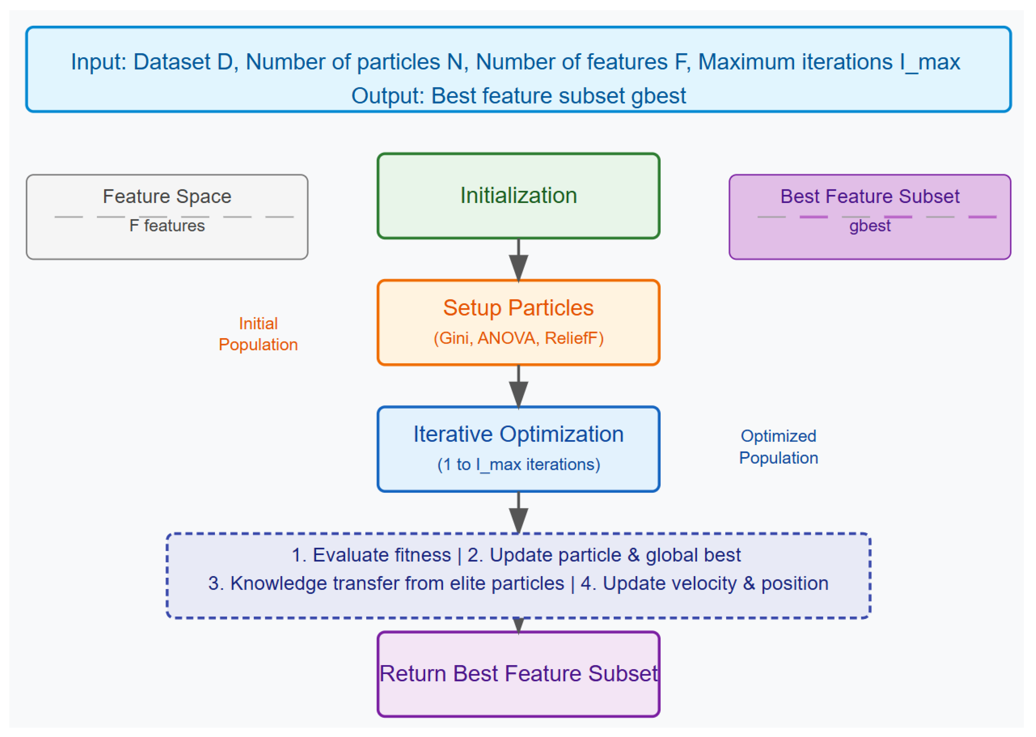
An overview of the proposed approach is shown in Figure 1. The two proposed algorithms have two goals in mind: (1) expansion of the search space using three filter-based methods to generate the particles and (2) using a fitness factor that weights accuracy and size of a feature set, including knowledge transfer, in order to prevent premature convergence. The figure as well as Algorithm 1 describe the approach.

The Guided Particle Swarm Optimization (PSO) algorithm for feature selection begins by initializing a swarm of particles, where each particle represents a potential subset of features. The goal of the algorithm is to identify the best feature subset that maximizes a fitness function, which likely measures the subset’s ability to accurately classify or predict outcomes based on the dataset provided.

Each particle in the swarm is assigned a random position (corresponding to a feature subset) and velocity, while the global best position, denoted as $gbest$, is initialized with an extremely high score, ensuring that any better solution will replace it. The initial positions of the particles are informed by three feature selection methods: Gini index, ANOVA, and ReliefF. Particles are divided equally among the positions computed by these methods, and their feature subsets are initialized using the knee point method, which balances the number of features with their relevance.

The algorithm then enters an iterative process, where it repeatedly evaluates and updates the particles over a series of iterations. During each iteration, the fitness of each particle’s feature subset is calculated. Fitness is calculated according to Equation (3):

$$fitness=\gamma ·CER+(1-\gamma )·(SFS/TFS)$$

(1)

where $\gamma$ is the weighting factor, $CER$ is the classification error rate, $SFS$ is the selected feature set, and $TFS$ is the total feature set.

If a particle’s current subset yields a better fitness score than its previously best-known score, the particle updates its best-known position. Similarly, if a particle’s fitness score is better than the global best score across the entire swarm, the global best position is updated.

The following velocity and position update equations are used:

$$v_i^{(t+1)}=\omega v_i^{\left(t\right)}+c_1{r}_1(pbes{t}_i-x_i^{\left(t\right)})+c_2{r}_2(gbest-x_i^{\left(t\right)})$$

(2)

$$s\left(v_i^{(t+1)}\right)={\displaystyle \frac{1}{1+e^{-v_i^{(t+1)}}}}$$

(3)

$$x_i^{(t+1)}=\left\{\begin{array}{cc}1,\hfill & \mathrm{if}r<s\left(v_i^{(t+1)}\right)\hfill \\ 0,\hfill & \mathrm{otherwise}\hfill \end{array}\right.$$

(4)

where $v_i^{(t+1)}$ is the updated velocity of particle i at time step $t+1$; $\omega$ is the inertia weight; $v_i^{\left(t\right)}$ is the previous velocity of the particle; $c_1$ and $c_2$ are the cognitive and social coefficients; $r_1,r_2\sim U(0,1)$ are random numbers sampled from a uniform distribution; $pbes{t}_i$ is the personal best position of particle i; $gbest$ is the global best position; $x_i^{\left(t\right)}$ is the current position of particle i; $s\left(v_i^{(t+1)}\right)$ is the sigmoid function applied to the velocity; $r\sim U(0,1)$ is a random number sampled from a uniform distribution; and $x_i^{(t+1)}$ is the updated binary position of the particle.

After evaluating all particles, the swarm is sorted based on their best scores. A subset of elite particles—those with the best performance—is identified, and knowledge from these elite particles is transferred to others in the swarm to guide the search towards more promising areas of the solution space; this is what we refer to as the knowledge transfer mechanism. Finally, each particle’s velocity and position are updated, allowing the swarm to explore new subsets of features while being influenced by both individual and collective experiences.

This process continues until the maximum number of iterations is reached, after which the algorithm returns the global best feature subset found, representing the most optimal selection of features according to the fitness function used.

Algorithm 1 Guided Particle Swarm Optimization for Feature Selection

1: Input: Dataset $\mathcal{D}$, Number of particles N, Number of features F, Maximum iterations $I_{max}$   2: Output: Best feature subset $\mathbf{gbest}$   3: Initialize particles with positions and velocities   4: Initialize global best position $\mathbf{gbest}$ and score $gbest\_score$ to infinity   5: for each particle i in the swarm do   6:   Compute Gini, ANOVA, and ReliefF positions for the dataset   7:   Divide particles equally among these positions   8:   Initialize feature subset ${\mathbf{fs}}_i$ using the knee point method   9: end for 10: for each iteration t from 1 to $I_{max}$ do 11:   for each particle i in the swarm do 12:     Evaluate fitness of ${\mathbf{fs}}_i$ using the fitness function 13:     if fitness is better than particle’s best score then 14:       Update particle’s best position and score 15:     end if 16:     if fitness is better than global best score then 17:       Update global best position and score 18:     end if 19:   end for 20:   Sort swarm based on particle best scores 21:   Update elite particles 22:   Transfer knowledge from elite particles to others 23:   for each particle i in the swarm do 24:     Update velocity and position of the particle 25:   end for 26: end for 27: return  $\mathbf{gbest}$

In terms of the complexity analysis, the time complexity is as follows:

$$O(I_{max}·N·M·F)$$

and the space complexity is as follows:

$$O(N·F)$$

where N is the number of particles in the swarm, F is the number of features in the dataset, M is the number of samples in the dataset, and $I_{max}$ is the maximum number of iterations.

The algorithm is computationally intensive for large datasets (large M and F) and large swarm sizes (N), but its linear scaling with respect to $I_{max}$ and N makes it manageable for large dataset sizes.

4. Experiments and Setup

This section first describes the datasets used followed by the descriptions of the comparison algorithms. Then, the evaluation measures are listed, and the experiments and results are shown and discussed.

4.1. Dataset Description

Twelve datasets have been used for the experiments. These have been extracted from the Cancer Genome Atlas (TCGA) [24]. TCGA is a pioneering cancer genomics initiative, and has molecularly characterized more than 20,000 primary cancer samples and corresponding normal tissues across 33 cancer types. This collaborative project, launched in 2006 by the National Cancer Institute (NCI) and the National Human Genome Research Institute, brought together experts from various fields and institutions.

Over the course of twelve years, TCGA produced more than 2.5 petabytes of data, encompassing genomic, epigenomic, transcriptomic, and proteomic information. This vast dataset, which has already contributed to advancements in cancer diagnosis, treatment, and prevention, continues to be publicly accessible to the research community.

The twelve datasets used are given in

Table 1. Description of the datasets.

Dataset	Rows (Samples)	Columns (Features)	Class 1	Class 2
CHOL	44	43,697	39	5
COAD	522	37,677	509	13
HNSC	564	35,958	535	29
KICH	91	43,806	60	31
KIRC	613	44,909	609	4
KIRP	322	44,874	236	86
LIHC	421	35,924	322	99
LUSC	553	44,894	494	59
PRAD	553	44,824	472	81
STAD	448	44,878	358	80
THCA	564	36,120	380	184
UCEC	588	36,086	345	243

. As one can see, the number of features vary between 35,924 to 44,909. Since we are investigating feature selection, these datasets are considered to be very large and appropriate for our experiments. The dataset abbreviations stand for Cholangiocarcinoma (CHOL), Colon Adenocarcinoma (COAD), Head and Neck Squamous Cell Carcinoma (HNSC), Kidney Renal Clear Cell Carcinoma (KIRC), Kidney Renal Papillary Cell Carcinoma (KIRP), Liver Hepatocellular Carcinoma (LIHC), Lung Squamous Cell Carcinoma (LUSC), Prostate Adenocarcinoma (PRAD), Stomach Adenocarcinoma (STAD), Thyroid Carcinoma (THCA), and Uterine Corpus Endometrial Carcinoma (UCEC). All datasets are binary with two classes: cancer or not cancer.

4.2. Comparison Approaches

The following comparison approaches have been used to select the best features. As for the classification portion, the K-Nearest Neighbor (KNN) has been used.

ANOVA (Analysis of Variance): ANOVA is a statistical method used to analyze the differences among group means among each other [25]. It determines whether there are any statistically significant differences between the means of independent groups by comparing the variability within groups to the variability between groups. Within feature selection, the ANOVA F-test identifies features that have significant differences across different classes and how different a feature is within its own class, helping to select the most relevant features for improving model performance. It uses ANOVA to select the top 10% of features based on their statistical significance, while retaining important features despite reducing dimensionality.

EN (Elastic Net): Elastic Net is an embedded method that combines both L1 (Lasso) and L2 (Ridge) embedded methods to enhance the performance of regression models [26], specifically their penalty coefficients. Elastic Net will be typically used in scenarios when the number of predictors exceeds the number of observations or when predictors are highly correlated. By linearly combining the penalties, Elastic Net encourages sparsity like lasso, which helps in variable selection, while also stabilizing the solution like ridge regression, which improves prediction accuracy.

BPSO (Binary PSO): BPSO was described in Section 2.

IG (Information Gain): Information gain is a criterion used in feature selection to measure how much information a given feature contributes to reducing uncertainty in a classification task. It is based on the concept of entropy from information theory, where entropy represents the amount of randomness or impurity in the dataset. The information gain of a feature is computed as the reduction in entropy achieved by partitioning the data based on that feature. A higher information gain indicates that the feature is more informative and useful for classification [27].

CS (Chi-Square Test): The Chi-Square Test is a filter type of the feature selection method. It evaluates each feature individually without considering a specific model. This method is effective across different models, as it is model-agnostic. The Chi-Square Test assigns each feature a Chi value based on its statistical relevance to the target variable. This approach is fast and efficient, particularly suitable for high-dimensional datasets. It works well with categorical datasets but can also handle qualitative data points [28].

CSA (ChiSimAnneal): ChiSimAnneal is a hybrid feature selection algorithm that combines the Chi-Square statistical test with a simulated annealing optimization strategy. The Chi-Square test evaluates the dependency between categorical features and the target variable, selecting features that exhibit strong statistical associations. Simulated annealing, a probabilistic optimization technique inspired by the annealing process in metallurgy, is then applied to refine the feature subset by exploring different combinations and avoiding local optima. This approach enhances the selection process by balancing exploration and exploitation, leading to an optimal subset of features that improve model performance [29].

PSO (4-2): PSO (4-2) allows particles to vary in length, reducing search space and improving PSO’s performance by focusing on relevant features. This technique enhances PSO’s ability to avoid local optima and produce high classification performance with fewer features in shorter time frames, as shown in tests on high-dimensional datasets [17], and was also described in Section 2.

RR (Ridge Regression): Ridge Regression integrates feature selection within the training process of a model. It is an example of an embedded method. During model training, Ridge Regression calculates coefficients for each feature, indicating their importance. Features with coefficients above a specified threshold (e.g., 0.2) are selected. This method is efficient and leverages the model’s learning process for feature selection. However, it may not eliminate irrelevant features entirely and requires careful parameter tuning to identify the most relevant features accurately [30].

GA (Genetic Algorithm): GA was described in Section 2.

IGPSO: IGPSO was described in Section 2.

ChaoticMap: ChaoticMap was described in Section 2.

VLPSO (Variable-length PSO): VLPSO was described in Section 2.

The last two algorithms listed, ChaoticMap and Variable-length PSO, were implemented for the comparison experiments; however, given the large dataset sizes, neither could be run due to their time complexity. However, all other comparison algorithms were included.

4.3. Algorithm Parameters

Table 2. Parameters used for the algorithms.

Algorithm	Parameters
GA	$num\_iterations=100$, $population\_size=30$, $mutation\_rate=0.01$, $crossover\_rate=0.9$
BPSO	$max\_iterations=min(50,num\_features\times 5)$, $num\_particles=min(30,num\_features\times 2)$, $w=0.5$, $c_1=2.0$, $c_2=2.0$
PSO(4-2)	$max\_iterations=100$, $num\_particles=30$, $w=0.7298$, $c_1=1.49618$, $c_2=1.49618$
IGPSO	$max\_iterations=100$, $num\_particles=30$, $w=0.9$, $c_1=2.0$, $c_2=2.0$, $hidden\_Layers=100$, $learning\_Rate=0.001$
GPSO	$max\_iterations=100$, $num\_particles=30$, $w=0.5$, $c_1=1.5$, $c_2=1.5$, $\gamma =0.95$

lists the parameters used for the experiments for the different algorithms. Please note that for IGPSO, the parameter values were set to those of GPSO as well as the other nature-inspired algorithms, in order to make sure that the same search effort was used.

4.4. Computing Infrastructure for Experiments

The experiments were conducted using the infrastructure of the Center for Computationally Assisted Science and Technology (CCAST), which offers advanced cyberinfrastructure for research and education at NDSU and beyond. CCAST manages and operates high-performance, cloud, and interactive computing resources, while also educating researchers on the effective and efficient utilization of these resources and other relevant topics in the computational science and engineering fields.

5. Results

This section presents the results of the experiments conducted.

Table 3. Accuracy.

Dataset	ANOVA	EN	BPSO	IG	CSA	PSO(4-2)	CS	RR	GA	IGPSO	GPSO
LUSC	0.918918919	0.927927928	0.933734940	0.937142857	0.928571429	0.854285714	0.928571429	0.928571429	1.000000000	0.957831330	0.999808907
PRAD	0.954954955	0.918918919	0.969879518	1.000000000	0.993630573	0.994394904	0.993630573	0.987261146	0.990500000	0.945783130	0.999864635
THCA	0.991150442	0.982300885	0.983764706	0.985176471	0.976470588	0.983058824	0.994117647	0.994117647	0.973500000	0.976470590	0.999402064
KICH	1.000000000	1.000000000	1.000000000	1.000000000	1.000000000	0.970000000	0.928571429	0.928571429	0.978960000	0.785714290	0.999807100
STAD	0.888888889	0.888888889	0.954666667	1.000000000	1.000000000	0.995000000	1.000000000	1.000000000	1.000000000	0.933333330	0.999893115
KIRP	0.861538462	0.707692308	0.894845361	0.874226804	0.845360825	0.860206186	0.824742268	0.824742268	0.793909656	0.927835050	0.998809975
KIRC	1.000000000	1.000000000	1.000000000	0.794645669	0.780157480	0.858267717	0.826771654	0.818897638	0.785860000	0.994565220	0.998207277
LIHC	0.858823529	0.858823529	0.851653543	0.944337349	0.913975904	0.913734940	0.903614458	0.897590361	0.931500000	0.929133860	0.998702470
HNSC	0.991150442	0.991150442	0.994117647	0.934216867	0.932289157	0.948192771	0.909638554	0.909638554	0.915300000	0.988235290	0.999074136
CHOL	1.000000000	1.000000000	1.000000000	0.938962963	0.957925926	0.935407407	0.888888889	0.888888889	0.893340000	0.928571430	0.998928181
UCEC	0.872881356	0.771186441	0.891073446	0.972705882	0.953411765	0.963529412	0.970588235	0.964705882	0.916820000	0.943502820	0.998391428
COAD	0.990476190	0.980952381	0.998980892	0.777853107	0.783954802	0.839774011	0.757062147	0.728813559	0.722020000	0.980891720	0.996616323

shows the accuracy results obtained running all algorithms on all datasets. The best values achieved for each dataset is highlighted in bold. As can be seen, our proposed algorithm as well as the BPSO obtains the highest accuracy for four datasets, the ANOVA, EN, and IG algorithms achieve the highest accuracy for three dataset, the CSA and GA algorithms for two datasets, and the CS and RR algorithms score best for one dataset.

As for the precision results given in

Table 4. Precision.

Dataset	ANOVA	EN	BPSO	IG	CSA	PSO(4-2)	CS	RR	GA	IGPSO	GPSO
LUSC	0.721428571	0.800925926	0.932653886	0.528571429	0.464285714	0.741915228	0.933673469	0.933673469	1.000000000	0.979452050	1.000000000
PRAD	0.913107511	0.957142857	0.965955305	1.000000000	0.996753247	0.994467040	0.993671933	0.987425519	0.995100000	0.951388890	1.000000000
THCA	0.993750000	0.987654321	0.999245283	0.992437775	0.988095238	0.982644656	0.994153298	0.994153298	0.486700000	0.980769230	1.000000000
KICH	1.000000000	1.000000000	1.000000000	1.000000000	1.000000000	0.972303770	0.935714286	0.935714286	0.971440000	0.642857140	1.000000000
STAD	0.813936249	0.826666667	0.930932182	1.000000000	1.000000000	0.991471723	1.000000000	1.000000000	1.000000000	0.800000000	1.000000000
KIRP	0.845025510	0.650000000	0.910681690	0.919573818	0.907432249	0.860018161	0.830402264	0.830402264	0.788695417	0.927536230	0.989361702
KIRC	1.000000000	1.000000000	1.000000000	0.891427300	0.885523547	0.872411609	0.859625305	0.854498957	0.809400000	0.925131000	0.927631579
LIHC	0.922077922	0.922077922	0.833752518	0.970447492	0.955748163	0.907109452	0.888522242	0.883924587	0.965320000	0.988505750	0.981132075
HNSC	0.995495495	0.995495495	1.000000000	0.963582103	0.962600204	0.948634266	0.918439994	0.918439994	0.955420000	0.833333330	0.984848485
CHOL	1.000000000	1.000000000	1.000000000	0.907256762	0.960964283	0.935505558	0.884848485	0.884848485	0.819760000	1.000000000	0.974025974
UCEC	0.918478261	0.870192308	0.864785550	0.980787469	0.968068064	0.964303382	0.971803597	0.965215686	0.935560000	0.944444440	0.987654321
COAD	0.995145631	0.990384615	1.000000000	0.864773098	0.867560880	0.869656895	0.827171729	0.813339203	0.850640000	0.666666670	0.877450980

, the proposed algorithm scores highest for seven datasets, BPSO scores best for five datasets, ANOVA and EN for three datasets, IG, CSA, and IGPSO for two datasets, and CS and RR for one dataset.

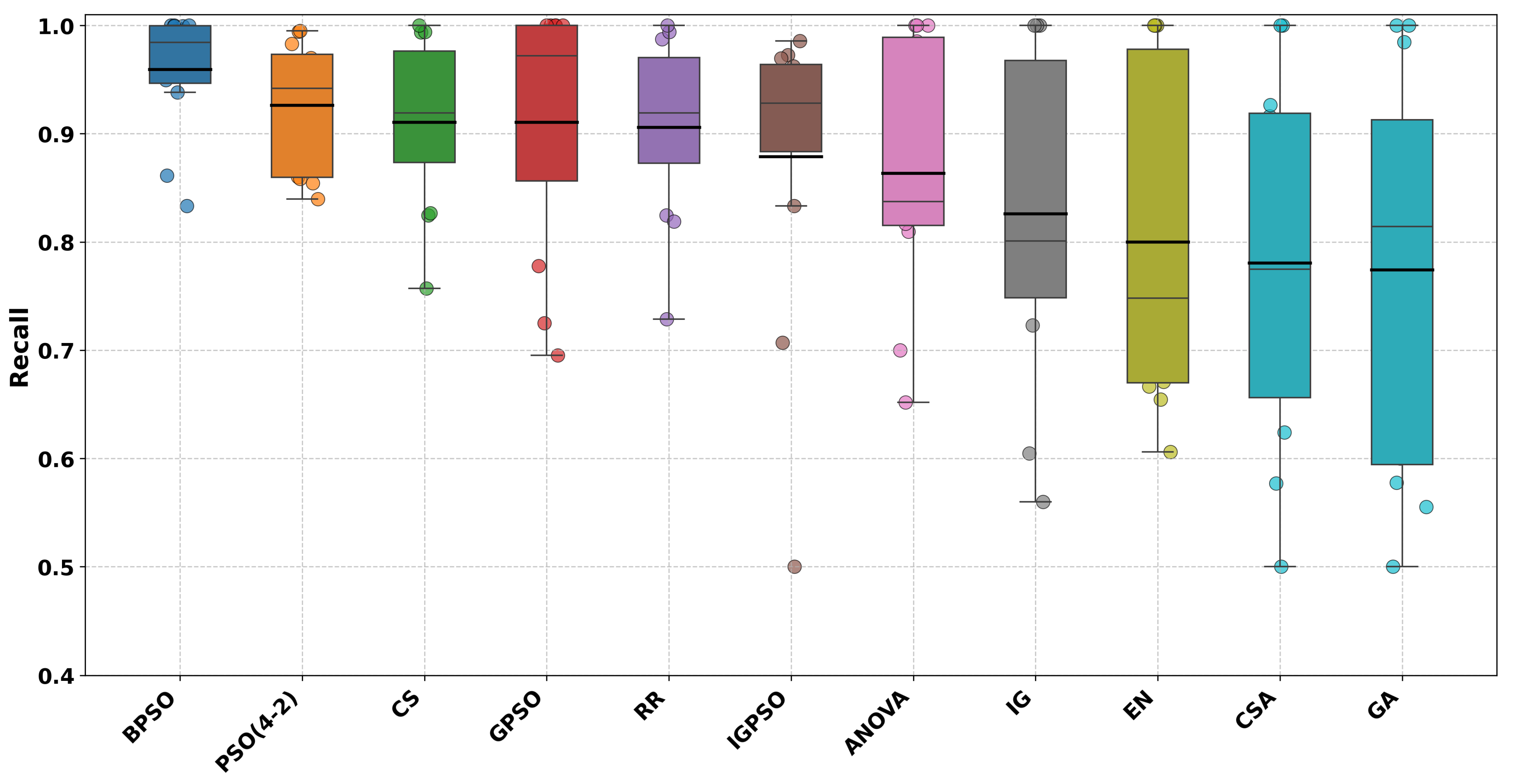
Next up are the recall results given in

Table 5. Recall.

Dataset	ANOVA	EN	BPSO	IG	CSA	PSO(4-2)	CS	RR	GA	IGPSO	GPSO
LUSC	0.651960784	0.606209150	0.997278912	0.560000000	0.500000000	0.854285714	0.928571429	0.928571429	1.000000000	0.972789120	1.000000000
PRAD	0.889583333	0.700000000	0.999424460	1.000000000	0.875000000	0.994394904	0.993630573	0.987261146	0.833300000	0.985611510	1.000000000
THCA	0.985294118	0.970588235	0.949629630	0.790000000	0.666666667	0.983058824	0.994117647	0.994117647	0.500000000	0.944444440	1.000000000
KICH	1.000000000	1.000000000	1.000000000	1.000000000	1.000000000	0.970000000	0.928571429	0.928571429	0.984600000	0.900000000	1.000000000
STAD	0.841257051	0.796132151	0.861333333	1.000000000	1.000000000	0.995000000	1.000000000	1.000000000	1.000000000	0.933333330	1.000000000
KIRP	0.809496568	0.654462243	0.938181818	0.804252199	0.758064516	0.860206186	0.824742268	0.824742268	0.795537907	0.969696970	0.973684211
KIRC	1.000000000	1.000000000	1.000000000	0.604848485	0.576969697	0.858267717	0.826771654	0.818897638	0.555380000	0.706954000	0.725000000
LIHC	0.700000000	0.700000000	0.999574468	0.756842105	0.624210526	0.913734940	0.903614458	0.897590361	0.577800000	0.914893620	0.777777778
HNSC	0.833333333	0.833333333	0.833333333	0.797777778	0.791851852	0.948192771	0.909638554	0.909638554	0.686660000	0.833333330	0.900000000
CHOL	1.000000000	1.000000000	1.000000000	0.919333333	0.916285714	0.935407407	0.888888889	0.888888889	0.889120000	0.923076920	0.882352941
UCEC	0.817073171	0.670731707	0.971698113	0.957037037	0.926666667	0.963529412	0.970588235	0.964705882	0.868440000	0.962264150	0.970588235
COAD	0.833333333	0.666666667	0.960000000	0.723098592	0.730704225	0.839774011	0.757062147	0.728813559	0.600040000	0.500000000	0.695121951

. As can be seen from the results in the table, GPSO again scores best for six datasets, followed by BPSO for five datasets, ANOVA for four datasets, EN and IG for three datasets, CSA and GA for two datasets, and PSO(4-2), CS, and RR for one dataset.

F1-scores are displayed in

Table 6. F1-score.

Dataset	ANOVA	EN	BPSO	IG	CSA	PSO(4-2)	CS	RR	GA	IGPSO	GPSO
LUSC	0.678260870	0.647619048	0.963853022	0.543703704	0.481481481	0.793330403	0.894179894	0.894179894	1.000000000	0.976109220	1.000000000
PRAD	0.900839736	0.763326226	0.982363144	1.000000000	0.926942764	0.993391544	0.993185988	0.985179364	0.897600000	0.968197880	1.000000000
THCA	0.989392659	0.978598485	0.973683196	0.861522292	0.743975904	0.981626562	0.993859207	0.993859207	0.493300000	0.962264150	1.000000000
KICH	1.000000000	1.000000000	1.000000000	1.000000000	1.000000000	0.969733992	0.926482874	0.926482874	0.976600000	0.750000000	1.000000000
STAD	0.826388889	0.809966216	0.893507467	1.000000000	1.000000000	0.993155412	1.000000000	1.000000000	1.000000000	0.861538460	1.000000000
KIRP	0.824060150	0.652014652	0.923813504	0.835557293	0.789293947	0.854992101	0.826748797	0.826748797	0.785075784	0.948148150	0.981110142
KIRC	1.000000000	1.000000000	1.000000000	0.612031700	0.568196159	0.835315666	0.792538433	0.780333793	0.541860000	0.760849000	0.771337735
LIHC	0.743460765	0.743460765	0.909023894	0.823405680	0.674311398	0.895034526	0.887988042	0.866681585	0.614740000	0.950276240	0.847527473
HNSC	0.897737557	0.897737557	0.909090909	0.854337133	0.849022355	0.944066609	0.894574359	0.894574359	0.746680000	0.833333330	0.936752137
CHOL	1.000000000	1.000000000	1.000000000	0.912996557	0.936060988	0.934552442	0.885130374	0.885130374	0.845520000	0.960000000	0.920000000
UCEC	0.843681003	0.679959819	0.914633668	0.967728257	0.943889994	0.963085341	0.970184608	0.964326252	0.893420000	0.953271030	0.978598485
COAD	0.897560976	0.745145631	0.977142857	0.730099899	0.738942797	0.830294654	0.724785912	0.684607063	0.578680000	0.571428570	0.710869352

. The table shows that the proposed algorithm, GPSO, obtains the best results for seven datasets followed by BPSO for five datasets, ANOVA, EN, and IG for three datasets, CSA and GA for two datasets, and PSO(4-2), CS, RR, and IGPSO for one dataset.

Figure 2, Figure 3, Figure 4 and Figure 5 show the accuracy, precision, recall, and F1-score results as box plots. Please note that numbers in bold indicate the best results.

In order to evaluate the different algorithms fairly, we are investigating their execution times as well.

Table 7. Execution time in seconds.

Dataset	ANOVA	EN	BPSO	IG	CSA	PSO(4-2)	CS	RR	GA	IGPSO	GPSO
LUSC	8.344077873	8.046691179	215.7868326	116.1854684	5.728559017	756.1332397	0.201476097	0.220444441	2061.760082	11,760.0400000	4727.830717
PRAD	8.281743498	8.080709219	71.73043895	119.4153876	6.43004775	579.0874655	0.162760019	0.233434916	1704.856312	8977.9900000	3468.037741
THCA	7.023365498	6.383810997	103.2177551	96.31234741	5.476798296	1001.062687	0.132241011	0.161518335	1496.199089	6857.7800000	3996.665895
KICH	1.902150631	1.893776417	43.85510159	62.40318799	3.061998367	128.7656426	0.074776888	0.030544043	513.1460321	1580.8700000	579.6270921
STAD	6.801307201	6.506551266	116.9085333	105.4947674	5.681056976	719.1091413	0.122227192	0.153008461	2035.534001	47,514.1000000	4584.996282
KIRP	5.174985647	4.774347305	96.44906592	91.59079242	4.331308365	558.1365902	0.105087519	0.092389584	1163.142314	3679.3100000	3026.042607
KIRC	9.101013899	8.821824551	219.8901556	125.1197939	4.912036657	439.8042846	0.197125673	0.276264906	1111.391231	6409.1700000	1929.743119
LIHC	5.159692764	5.282177925	93.40946531	81.89385223	4.901816607	386.6665111	0.131872177	0.109116077	1556.080096	14,811.1700000	2382.776136
HNSC	6.716423035	6.691006422	177.0269773	93.53505182	4.944217443	505.0531957	0.147221565	0.171553373	868.4110465	12,283.4200000	2802.933625
CHOL	1.191920996	1.373466492	23.94001317	57.90781331	2.576358557	67.65457416	0.068276167	0.013371468	184.4370654	1768.1600000	393.1442497
UCEC	6.922133207	6.824393749	27.79974627	97.69451523	5.227145195	538.350606	0.133640528	0.191025019	1747.461532	5680.6000000	5587.026212
COAD	6.522175074	6.235757828	106.4919822	93.48602939	4.649344683	232.7946894	0.139748335	0.172054291	1252.530542	8167.4100000	1559.296618

lists the running time/execution time of all algorithms run on all datasets. As can be seen, the fastest algorithms are CS followed by RR taking our proposed algorithm. However, as we have seen, both algorithms do not score very highly in terms of accuracy, precision, recall, and F1-score. The IGPSO takes the longest, with an average of 10,790.84 s (179.85 min), followed by our algorithm, with an average of 2919.84 s (48.66 min). However, our algorithm scores overall better based on the other measures. Not unexpected, the third slowest algorithm is GA followed by PSO(4-2) and BPSO.

In terms of the number of features used and selected during the feature selection process,

Table 8. Number of features.

Dataset	All	ANOVA	EN	BPSO	IG	CSA	PSO(4-2)	CS	RR	GA	IGPSO	GPSO
LUSC	43,696	4489	4489	11,388	13,968	4336	4369	10,924	4589	21,833	37	167
PRAD	37,676	4482	4482	3685	12,137	3033	3767	9419	7753	18,813	16	102
THCA	35,957	3611	3611	4801	10,480	4397	4144	8989	7050	17,952	200	430
KICH	43,805	4380	4380	21,819	15,846	7028	4380	10,951	5689	21,864	2	169
STAD	44,908	4487	4487	6593	13,185	2505	4490	11,227	7052	22,496	31,792	96
KIRP	44,873	4487	4487	22,245	16,002	6531	7595	11,218	6660	44,873	186	1068
KIRC	35,923	4490	4490	22,335	11,919	5722	4763	8980	7286	17,863	1	1288
LIHC	44,893	3592	3592	6747	15,401	5206	3750	11,223	7198	22,360	1314	1165
HNSC	44,823	3595	3595	18,188	13,359	6116	6755	11,205	7151	22,374	12	830
CHOL	44,877	4369	4369	21,787	14,843	5151	7188	11,219	6932	22,361	2	962
UCEC	36,119	3608	3608	241	11,021	5159	5510	9029	7397	17,976	2207	1162
COAD	36,085	3767	3767	18,691	13,019	5483	4060	9021	7636	18,011	2	2442

shows the results. As can be seen, IGPSO uses by far the fewest numbers of features during the process followed by GPSO. All other algorithms select and use more features for the classification task.

Table 9. Mann–Whitney U test results—accuracy.

Algorithm	U Statistic	p-Value
ANOVA	36.0	0.0402
EN	36.0	0.0402
BPSO	42.0	0.0883
IG	36.0	0.0402
CSA	24.0	0.0061
PSO(4-2)	0.0	<0.0001
CS	12.0	0.0006
RR	12.0	0.0006
GA	24.0	0.0061
IGPSO	0.0	<0.0001

,

Table 10. Mann–Whitney U test results—precision.

Algorithm	U Statistic	p-Value
ANOVA	52.5	0.2638
EN	51.0	0.2278
BPSO	61.5	0.5490
IG	45.5	0.1262
CSA	42.0	0.0847
PSO(4-2)	27.0	0.0099
CS	32.5	0.0233
RR	30.5	0.0171
GA	34.0	0.0284
IGPSO	27.5	0.0105

,

Table 11. Mann–Whitney U test results—recall.

Algorithm	U Statistic	p-Value
ANOVA	55.5	0.3465
EN	42.0	0.0826
BPSO	76.5	0.8140
IG	50.5	0.2168
CSA	39.0	0.0575
PSO(4-2)	58.0	0.4337
CS	61.0	0.5411
RR	59.5	0.4850
GA	39.0	0.0575
IGPSO	51.5	0.2460

and

Table 12. Mann–Whitney U test results—F1-score.

Algorithm	U Statistic	p-Value
ANOVA	51.5	0.2394
EN	42.0	0.0826
BPSO	66.5	0.7687
IG	47.5	0.1581
CSA	39.0	0.0575
PSO(4-2)	52.0	0.2582
CS	49.5	0.2006
RR	48.5	0.1809
GA	35.0	0.0329
IGPSO	42.0	0.0871

show the results of the Mann–Whitney U Test comparing GPSO with all other algorithms in terms of accuracy, precision, recall, and F1-score. The analysis revealed several findings regarding the performance of GPSO compared to other algorithms.

Based on these results, GPSO shows statistically significant differences in accuracy compared to 9 out of the 10 other algorithms, with only BPSO showing a non-significant difference (though still trending toward significance with p = 0.0883). The very low p-values against several algorithms (particularly PSO(4-2) and IGPSO) suggest that GPSO performs either significantly better or significantly worse than these algorithms.

For precision, GPSO shows statistically significant differences compared to 5 out of the 10 other algorithms (PSO(4-2), CS, RR, GA, and IGPSO). The differences with CSA are close to significance (p = 0.0847). The remaining algorithms (ANOVA, EN, BPSO, and IG) do not show statistically significant differences in precision when compared with GPSO.

For recall metrics, GPSO does not show statistically significant differences compared to any of the 10 other algorithms at the conventional significance level of $\alpha$ = 0.05. However, three algorithms show trends toward significance (p < 0.10):

• EN vs. GPSO (p = 0.0826);
• CSA vs. GPSO (p = 0.0575);
• GA vs. GPSO (p = 0.0575).

This suggests that while there may be some differences in recall performance between GPSO and these three algorithms, the differences are not strong enough to be considered statistically significant with the current sample size and at the conventional significance threshold.

In summary, GPSO shows a statistically significant difference only when compared to GA (p = 0.0329). It shows marginally significant differences (p < 0.1) when compared to EN, CSA, and IGPSO. For all other algorithms, there are no statistically significant differences in performance based on the provided test results.

6. Conclusions

In this paper, we proposed a feature selection method based on Particle Swarm Optimization. The proposed algorithm makes use of a guided particle scheme whereby three filter-based methods are incorporated. The proposed algorithm addressed the issue of premature convergence to global optima compared to other PSO feature-based methods by the expansion of the search space using three filter-based methods to generate particles, and by using a fitness factor that weights accuracy and size of feature set including knowledge transfer. The proposed method was compared to state-of-the-art feature selection algorithms. ANOVA, EN, BPSO, IG, CSA, PSO(4-2), CS, RR, GA, and IGPSO were implemented and experimented with. The 12 genome datasets we used included up to 44,909 features, which is consider high-dimensional data. The results as well as statistical analysis show that the proposed algorithm compares better to other state-of-the-art feature selection algorithms. In summary, GPSO achieves competitive or better accuracy and precision compared to most algorithms, with similar recall and some variation in F1-score. This indicates its strength in balancing accuracy and precision while maintaining performance on other metrics.

Future work will involve conducting additional experiments to further evaluate the robustness and adaptability of the knowledge-transfer mechanism across diverse datasets and problem domains. This should include fine-tuning the parameters and design of the mechanism to enhance its effectiveness and efficiency. Additionally, a systematic comparison with alternative knowledge-transfer solutions, such as transfer learning frameworks, meta-learning approaches, and domain adaptation techniques, could be performed. Moreover, exploring hybrid approaches that combine multiple knowledge-transfer techniques may lead to improved performance.