Improved Trimming Ant Colony Optimization Algorithm for Mobile Robot Path Planning

Abstract

Traditional ant colony algorithms for mobile robot path planning often suffer from slow convergence, susceptibility to local optima, and low search efficiency, limiting their applicability in dynamic and complex environments. To address these challenges, this paper proposes an improved trimming ant colony optimization (ITACO) algorithm. The method introduces a dynamic weighting factor into the state transition probability formula to balance global exploration and local exploitation, effectively avoiding local optima. Additionally, the traditional heuristic function is replaced with an artificial potential field attraction function, dynamically adjusting the potential field strength to enhance search efficiency. A path-length-dependent pheromone increment mechanism is also proposed to accelerate convergence, while a triangular pruning strategy is employed to remove redundant path nodes and shorten the optimal path length. Simulation experiments show that the ITACO algorithm improves the path length by up to 62.86% compared to the classical ACO algorithm. The ITACO algorithm improves the path length by 6.68% compared to the latest related research results. These improvements highlight the ITACO algorithm as an efficient and reliable solution for mobile robot path planning in challenging scenarios.

1. Introduction

Mobile robots have significant advantages in improving work efficiency, reducing labor intensity, and optimizing production processes. They are widely used in various fields such as home services, industrial manufacturing, medical care, mining and resource exploration, logistics and transportation, military reconnaissance, and space exploration. Examples include cleaning robots, warehouse robots, mining robots, and drones [1,2,3,4,5,6,7,8,9,10]. Path planning, as one of the core technologies for the autonomous navigation of mobile robots, plays a decisive role in the operational efficiency, safety, and motion control of robots. Therefore, the performance of path planning algorithms is an important indicator of the intelligence level of mobile robots and a hot topic in robotics research worldwide.

Traditional path planning algorithms, such as Dijkstra’s algorithm [11], A* algorithm [12,13,14], Rapidly-exploring Random Tree (RRT) [15], artificial neural networks (ANNs) [16], Dynamic Window Approach (DWA) [13,14], and Artificial Potential Field (APF) [17], have significant limitations in practical applications. For example, Dijkstra’s algorithm has high computational complexity and long search times; the A* algorithm often generates paths with many turns and low smoothness; the RRT has slow convergence and strong randomness in path generation; ANNs require long training times and are prone to falling into local optima; the DWA is sensitive to parameters and has high computational complexity; and the APF is prone to local optima and target unreachability issues. These limitations make it difficult for traditional algorithms to meet the real-time and efficiency requirements of path planning in complex environments.

Compared to the traditional algorithms, swarm intelligence algorithms, which simulate the collaborative behavior of biological groups, have shown significant advantages in path planning in complex environments. For example, the Ant Colony Optimization (ACO) algorithm guides path search through pheromones, demonstrating strong global search capabilities [18]; the Particle Swarm Optimization (PSO) algorithm achieves efficient optimization through information sharing among particles [19]; the Grey Wolf Optimizer (GWO) approximates the optimal solution through the social hierarchy of grey wolves [20]; the Artificial Bee Colony (ABC) algorithm enhances search efficiency through the division of labor among bees [21]; and the Dung Beetle Optimization (DBO) algorithm, inspired by the natural foraging and rolling behaviors of dung beetles, demonstrates strong optimization capabilities and fast convergence [22]. Among these, the ACO algorithm is widely adopted in combinatorial optimization problems, such as path planning and scheduling, due to its robust performance [23]. Nevertheless, in certain technical object optimal design problems, algorithms like PSO and GWO may outperform ACO.

While ACO has demonstrated strong performance in combinatorial optimization, it is important to acknowledge its limitations. Traditional ACO algorithms still suffer from problems such as local optima and poor convergence. To address these issues, researchers [24,25,26,27,28,29,30,31,32] have proposed various improvement methods. Such research has significantly enhanced the path smoothness, convergence speed, and global search capabilities of ACO algorithms through strategies such as optimized pheromone initialization (e.g., non-uniform distribution, reinforcement of key nodes), improved heuristic functions (incorporating turning penalties and distance factors), dynamically adjusted evaporation factors, reward–punishment mechanisms, integration with elite/Max–Min models, and multi-objective optimization (balancing path length, safety, and energy consumption). However, further improvements are still needed in real-time performance, dynamic adaptability, and the avoidance of local optima in complex environments.

To address the above issues, this paper proposes an Improved Trimming Ant Colony Optimization (ITACO) algorithm. The algorithm introduces a dynamic weighting factor in the state transition formula to balance global exploration and local exploitation, effectively avoiding local optima. It replaces the traditional heuristic function with an artificial potential field attraction function, significantly improving search efficiency. A path-length-dependent pheromone increment mechanism is proposed to enhance the pheromone update rule, further accelerating convergence. Finally, redundant path nodes are removed through a triangular pruning strategy, shortening the optimal path length. Simulation results show that, compared to the traditional ACO algorithms, the proposed algorithm significantly improves global search capabilities, search efficiency, and convergence speed, particularly exceling in complex environments and large-scale maps, and is suitable for modern applications such as autonomous robots and UAV navigation.

The remainder of this paper is as follows: Section 2 reviews the classic ACO. Section 3 introduces ITACO. Section 4 details the ITACO algorithm’s implementation. Section 5 presents the experimental setup, performance tests, and verification of ITACO’s effectiveness and superiority. Section 6 concludes the paper and discusses future research directions.

2. Traditional Ant Colony Optimization (ACO) Algorithm

The Ant Colony Optimization algorithm is a bio-inspired optimization algorithm that mimics the foraging behavior of ants in nature [33]. During foraging, ants deposit pheromones along the paths they traverse, which other ants can sense and follow probabilistically. Paths with higher pheromone concentrations tend to attract more ants, creating a positive feedback mechanism that reinforces the pheromone levels on these paths, while paths with fewer ants experience a gradual decrease in pheromone concentration over time. This collective behavior enables ants to efficiently discover the shortest path between their nest and a food source. The two fundamental components of the Ant Colony Optimization algorithm are state transition probability and pheromone update.

2.1. State Transition Probability

Let the total number of ants in the colony be M, the number of nodes be n, and the total number of iterations be T. Ant k (k = 1, 2, …, M) determines its next node to visit based on the pheromone concentration on the paths between the nodes. At the initial time step, the pheromone concentration on the paths between all nodes is set to the same value, denoted as ${\tau }_{ij}\left(t\right)={\tau }_0$. Let $P_{ij}^k\left(t\right)$ denote the probability that ant k moves from node i to node j at the t-th iteration.The formula for $P_{ij}^k\left(t\right)$ is given by Equation (1).

$$P_{ij}^k\left(t\right)=\left\{\begin{array}{c}{\displaystyle \frac{{\left[{\mathit{\tau }}_{\mathit{i}\mathit{j}}\left(\mathit{t}\right)\right]}^{\mathit{\alpha }}\cdot {\left[{\mathit{\eta }}_{\mathit{i}\mathit{j}}\left(\mathit{t}\right)\right]}^{\mathit{\beta }}}{\sum _{\mathit{j}\in {\mathit{a}}_{\mathit{k}}}{\left[{\mathit{\tau }}_{\mathit{i}\mathit{j}}\left(\mathit{t}\right)\right]}^{\mathit{\alpha }}\cdot {\left[{\mathit{\eta }}_{\mathit{i}\mathit{j}}\left(\mathit{t}\right)\right]}^{\mathit{\beta }}}} ,j\in a_k\\ 0 , otherwise\end{array}\right.$$

(1)

$${\eta }_{ij}\left(t\right)={\displaystyle \frac{1}{d_{ij}}}$$

(2)

In Equation (1), ${\tau }_{ij}\left(t\right)$ represents the pheromone concentration retained on the path from node i to node j at the t-th iteration, and ${\eta }_{ij}\left(t\right)$ denotes the heuristic information from node i to node j at the t-th iteration. The formula for ${\eta }_{ij}\left(t\right)$ is given by Equation (2), where $d_{ij}(i,j=1,2,\dots n)$ represents the Euclidean distance between node i and node j. The set $a_k$ denotes the collection of node positions that ant k may potentially move to from node i. The parameter α is the pheromone heuristic factor, which reflects the importance of pheromone concentration in path selection, and the ants tend to choose the path with large pheromone concentration; β is the expectation heuristic factor, indicating the significance of heuristic information in path selection, and the ants tend to choose nodes that are close to the goal point.

2.2. Pheromone Update

Ants leave pheromones on the paths they take, and the pheromones volatilize over time, changing the probability that a path will be chosen. Therefore, when the ant finds a reachable path, it needs to update the pheromone value of each edge contained in the path based on the total length of the path. After the t-th iteration of ants complete the search, the pheromone updating strategy shown in Equation (3) is used to adjust the pheromone concentration on the paths that the ants travel.

$${\tau }_{ij}(t)=(1-\rho )\cdot {\tau }_{ij}(t-1)+\rho \Delta {\tau }_{ij}(t)$$

(3)

In Equation (3), ρ is the pheromone evaporation coefficient, generally between 0 and 1, and $\Delta {\tau }_{ij}(t)$ represents the additional pheromone deposited on the path after the current iteration. The formula for $\Delta {\tau }_{ij}(t)$ is given by Equation (4).

$$\Delta {\tau }_{ij}\left(t\right)=\left\{\begin{array}{c}{\displaystyle \frac{Q}{L_k}}\\ 0\end{array}\right.{\displaystyle \genfrac{}{}{0pt}{}{ ,\mathrm{if}\mathrm{ant}k\mathrm{travels}\mathrm{through}\mathrm{path}\left(i,j\right)}{ , \mathrm{otherwise}}}$$

(4)

In Equation (4), $Q$ represents the pheromone intensity coefficient, and $L_k$ denotes the total path length traversed by the k-th ant to reach the destination. As indicated by Equation (4), the shorter the path length $L_k$ that an ant travels during path planning, the more pheromone is deposited on that path. This increased pheromone concentration makes the path more attractive to other ants, thereby creating a positive feedback loop.

3. Improved Trimming Ant Colony Optimization (ITACO) Algorithm

3.1. Improved State Transition Probability Formula

The traditional ant colony algorithm possesses several advantages, including local obstacle avoidance, strong robustness, positive feedback, and parallelism. However, it also suffers from certain limitations, such as slow convergence speed and a tendency to fall into local optima [34,35,36]. To overcome these limitations, this paper introduces a weighting factor $\partial \left(\partial \in \left(0,1\right)\right)$ into the state transition probability formula. The enhanced state transition formula is presented in Equations (5) and (6).

$$P_{ij}^k\left(t\right)=\left\{\begin{array}{c}\partial \cdot {\displaystyle \frac{{\left[{\mathit{\tau }}_{\mathit{i}\mathit{j}}\left(\mathit{t}\right)\right]}^{\mathit{\alpha }}\cdot {\left[{\mathit{\eta }}_{\mathit{i}\mathit{j}}\left(\mathit{t}\right)\right]}^{\mathit{\beta }}}{\sum _{k\in \left\{N-tab{u}_k\right\}}{\left[{\mathit{\tau }}_{\mathit{i}j}\left(\mathit{t}\right)\right]}^{\mathit{\alpha }}\cdot {\left[{\mathit{\eta }}_{\mathit{i}j}\left(\mathit{t}\right)\right]}^{\mathit{\beta }}}} , j\in \left\{N-tab{u}_k\right\}\\ 0 , other\end{array}\right.$$

(5)

$$\partial =\mathrm{s}\mathrm{i}\mathrm{n}\left({\displaystyle \frac{\pi t}{2T}}\right)$$

(6)

In the early stages of the algorithm, ants exhibit strong exploratory behavior, as the algorithm has not yet determined which path or solution is better. At this stage, the value of $\partial$ is relatively small, allowing the heuristic function to exert a greater influence on the selection probability. This encourages ants to extensively explore a wide range of paths or solution spaces, increasing the likelihood of discovering high-quality solutions and preventing premature convergence to local optima. In the later stages of the algorithm, ants have accumulated pheromone information about good paths through earlier exploration. The value of $\partial$ increases, enhancing the influence of pheromone concentration on the selection probability. As a result, the algorithm becomes more inclined to exploit the high-quality paths already identified, which accelerates convergence to the global optimum or a near-optimal solution.

This dynamic weighting mechanism also enables the algorithm to handle other optimization problems, such as coverage maximization tasks, by changing path minimization goal to coverage maximization goal. For applications requiring area coverage (e.g., cleaning or surveillance), the heuristic component ${\eta }_{\mathrm{i}\mathrm{j}}$ can be modified as the inverse of the visitation frequency to prioritize unvisited regions. Combined with our pruning strategy (Section 3.3), this adaptation can mimic the memory effect of chaos-based methods like P-RBMCA [37], while retaining convergence guarantees of ITACO.

Additionally, this paper employs an artificial potential field as the heuristic function to replace the traditional heuristic function, thereby further enhancing the algorithm’s convergence speed and optimization capability. The artificial potential field operates on the principle that a virtual potential field exists within the grid map [38]. In a virtual potential field, the potential energy to which the robot is subjected is proportional to the distance between the robot and the target point. Under the influence of the attractive field, the robot is continuously drawn toward the target point, enabling the planning of collision-free paths. The heuristic function incorporating the attractive potential field is defined in Equation (7), and the potential field attraction formula is given in Equation (8), as follows:

$${\eta }_{ij}={\left({\displaystyle \frac{1}{2}}\right)}^{fa}\cdot {\displaystyle \frac{1}{{\left({\left(x_i-x_g\right)}^2+{\left(y_i-y_g\right)}^2\right)}^{0.5}}}$$

(7)

$$fa=\sigma \cdot {\left(x_i-x_g\right)}^2+{\left(y_i-y_g\right)}^2$$

(8)

where $\sigma$ represents a potential field constant greater than 0, which is used to adjust the intensity of the potential field; $\left(x_i,y_i\right)$ represents the current coordinates of the robot; and $\left(x_g,y_g\right)$ denotes the coordinates of the target point.

A larger $\sigma$ results in a stronger attractive force of the potential field, promoting a broader search range for the algorithm, whereas a smaller $\sigma$ leads to a weaker attractive force, enabling a local optimization of the path. To balance global exploration and local exploitation, $\sigma$ is set to 10 when the number of iterations is less than or equal to $T/2$, ensuring effective global guidance. When the number of iterations exceeds $T/2$, $\sigma$ is set to 2, allowing for a more precise adjustment of the ants’ paths.

The integration of the weighting factor and the artificial potential field into the ant colony algorithm not only enhances exploration in the early stages but also improves exploitation in the later stages, ensuring faster convergence, avoiding local optima, and achieving superior optimization results.

3.2. Improved Pheromone Increment Update Strategy

In traditional ant colony algorithms, all ants share the same pheromone increment update rule, which limits the algorithm’s ability to converge quickly. To overcome this limitation, this paper introduces a path-length-dependent pheromone increment mechanism to enhance the update rule, enabling faster and more efficient convergence.

After each iteration, ants that are trapped in deadlock are discarded, and the average path length of ants that successfully reach the target node is calculated. The pheromone increment on the path planned by the optimal ant is updated according to Equation (9). By intensifying the pheromone concentration on the optimal path, the algorithm reinforces its attractiveness in subsequent iterations, thereby accelerating convergence toward high-quality solutions.

$$\Delta {\tau }_{ij}={\lambda }_1{\displaystyle \frac{Q}{L_k}}, L_k=L_{\mathrm{b}\mathrm{e}\mathrm{s}\mathrm{t}}$$

(9)

For ants whose path lengths are longer than that of the optimal ant but still shorter than the average path length, the pheromone increment on their paths is updated according to Equation (10). This approach ensures that paths with moderate performance receive a balanced pheromone update, maintaining diversity in the search process without overly rewarding suboptimal solutions.

$$\Delta {\tau }_{ij}={\lambda }_2{\displaystyle \frac{Q}{L_k}}, L_{\mathrm{b}\mathrm{e}\mathrm{s}\mathrm{t}}<L_k\le \bar{L}$$

(10)

In cases where an ant’s path length exceeds the average path length of the current iteration, the pheromone increment on that path is updated according to Equation (11). By reducing the pheromone increment for inferior solutions, the algorithm minimizes the misleading influence of poorer paths on subsequent iterations, thereby improving the overall efficiency and accuracy of the search process.

$$\Delta {\tau }_{ij}={\lambda }_3{\displaystyle \frac{Q}{L_k}}, L_k>\bar{L}$$

(11)

where the following are expressed:

• $Q$ is the pheromone intensity coefficient;
• $L_{\mathrm{b}\mathrm{e}\mathrm{s}\mathrm{t}}$ is the length of the best path in the current iteration;
• $\bar{L}$ is the average path length of successful ants;
• ${\lambda }_1$, ${\lambda }_2$, ${\lambda }_3$ are positive constants satisfying ${\lambda }_1$>${\lambda }_2$>${\lambda }_3$> 0. In this paper, ${\lambda }_1$ = 2, ${\lambda }_2$ = 1.5, and ${\lambda }_3$ = 0.5.

This adaptive pheromone update mechanism dynamically prioritizes high-quality solutions and discourages the exploration of less promising paths. By assigning differentiated pheromone increments based on path quality, the algorithm not only accelerates convergence to the optimal solution but also maintains a balanced exploration–exploitation trade-off, leading to improved optimization outcomes.

The same framework can extend to other optimization problems, such as path length maximization, by inverting the pheromone update rule to reward longer valid paths.

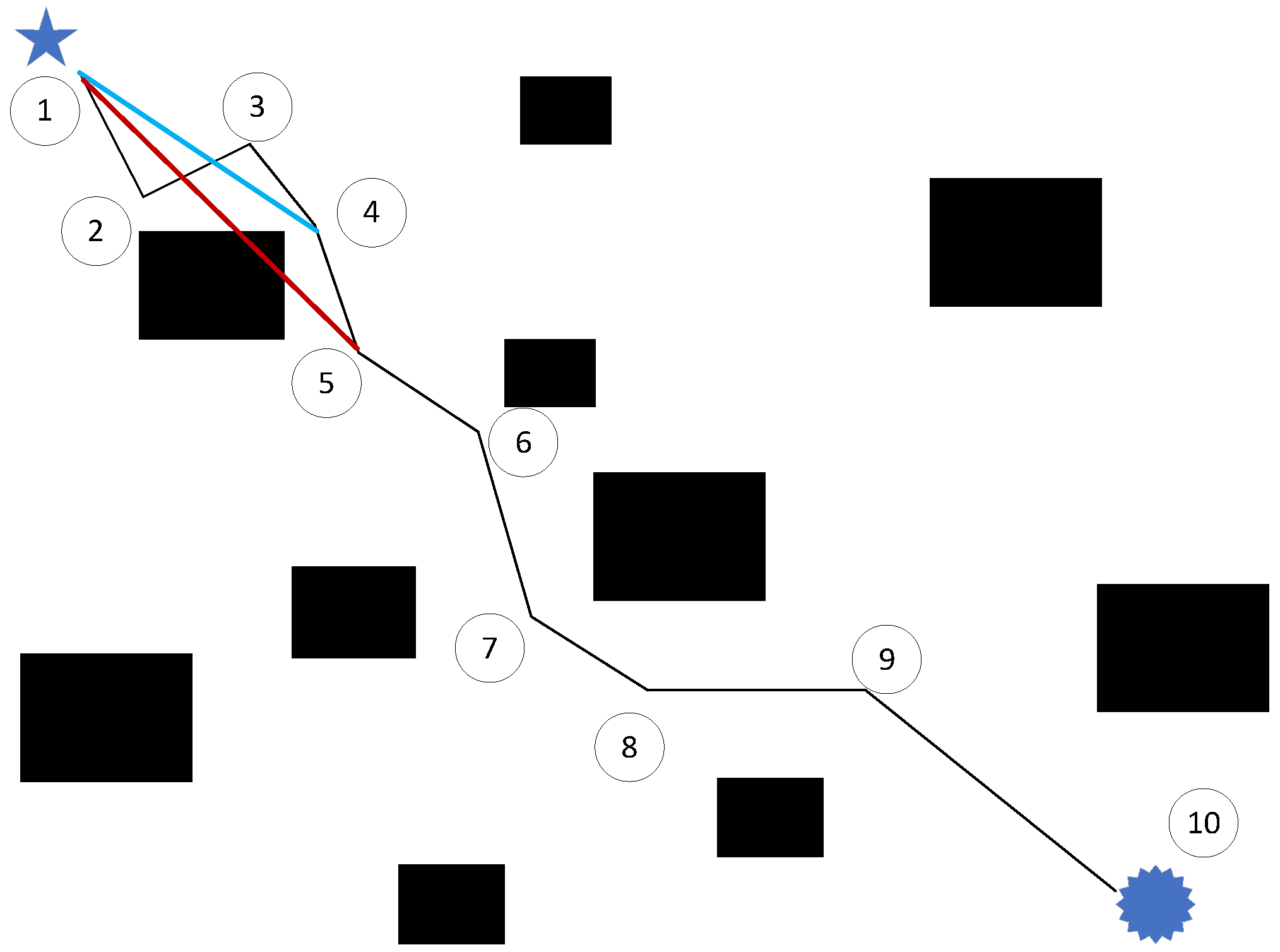
3.3. Triangular Trimming Path Optimization

Triangular pruning utilizes the principle that the sum of the lengths of any two sides of a triangle is greater than the length of the remaining side. In this paper, triangular pruning is introduced to further optimize the paths generated by the ant colony optimization algorithm. By traversing all nodes on the path, redundant nodes are removed to shorten the path length. In path planning, the application of triangular pruning primarily involves eliminating triangular regions that cannot possibly be part of the optimal path, thereby reducing the search space and computational load, and improving the efficiency of path planning.

The main idea is to connect the first node with the second node. If there are no obstacles between them, the second node is discarded. Next, the first node is connected to the third node. If there are no obstacles between them, the third node is discarded. This process continues sequentially, connecting the first node with the fourth node, and so on, until an obstacle is encountered between the first node and the node to be connected. The node immediately before the obstacle is then connected to the first node to form a new path. This node becomes the new starting point, and the process is repeated until the final node is reached. The pruning process is illustrated in Figure 1.

In Figure 1, graphical elements are defined as:

• Black squares: Obstacle locations
• Circled numbers: Path nodes (1, 2, 3,…)
• Black solid line: Initial candidate path
• Blue bold line: Optimized path after pruning
• Red dashed line: Invalid obstacle-crossing paths

The path optimization process through the triangular pruning technique:

• The algorithm begins by connecting nodes sequentially (1→2→3→4→5…)
• When the direct connection between nodes 1→5 fails due to obstacle interference:

  (a)

  The system backtracks to the last viable node (node 4)

  (b)

  Establishes new valid segment (1→4)

  (c)

  Continues connection from node 4 onward

• This pruning process iterates until reaching the final node

The introduction of triangular pruning effectively reduces redundant path length in path planning.

4. Implementation of the Improved Ant Colony Optimization Algorithm

The specific steps of the improved ant colony optimization algorithm are as follows:

Step 1: Initialization: Construct a 2D static grid environment map and initialize parameters, including the number of ants M, start node S, target node E, maximum iterations T, pheromone evaporation coefficient ρ, pheromone importance factor α, and heuristic importance factor β.

Step 2: Ant Path Selection: Place M ants at the start node S. Initialize the tabu list and add S to it. Use Equation (5) to select the next node j, add j to the tabu list, and update the path length. Repeat this process until the ants reach the target node or encounter a deadlock.

Step 3: Pheromone Increment Update: After each iteration, discard ants that fail to reach the target node. For successful ants, update the pheromone increment using Equations (9)–(11).

Step 4: Pheromone Concentration Update: Update the pheromone concentration using Equation (3).

Step 5: Output the Pre-Trimming Path: Repeat Steps 2–4 until the maximum number of iterations is reached. Output the pre-trimmed path.

Step 6: Triangular Trimming: Perform triangular trimming on the output path from Step 5. Remove redundant nodes and connect the remaining nodes to obtain the final optimal path.

The flow of the improved ACO algorithm is shown in Figure 2.

Our improvements to ACO include the state transfer strategy, the pheromone incremental update strategy, and path pruning. Since the state transfer strategy and the pheromone incremental update strategy just replace the original ones, and the time complexity of path pruning is at a linear level, the time complexity of ITACO is at the same level as that of ACO.

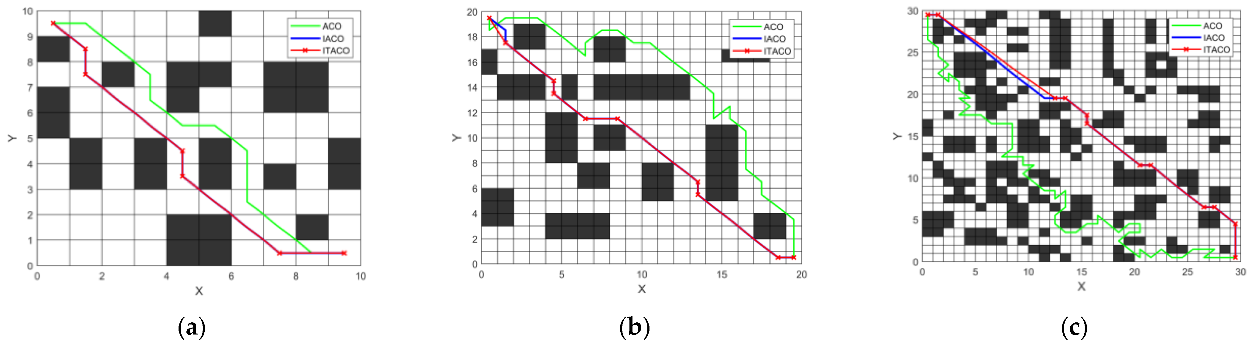
5. Experimental Simulation and Results

5.1. Simulation Setup

To validate the performance of the improved ant colony algorithm, this paper first tests the optimization capability of the algorithm using six classic international benchmark functions. Then, simulation experiments are conducted on 2D static grid maps with sizes of 10 × 10, 20 × 20, and 30 × 30. The obstacle configurations were generated using a predefined method to establish standard test cases. This approach ensures reproducibility and facilitates a direct comparison with the existing algorithms.

The performance of the algorithm is compared and analyzed in terms of path planning effectiveness, convergence speed, number of iterations, computational time, and path length. For ease of reference, the following abbreviations are used:

• ITACO: improved ant colony optimization algorithm proposed in this paper;
• IACO: improved algorithm without triangular pruning;
• ACO: classic ant colony algorithm.

The experimental parameter settings are shown in

Table 1. Parameter settings for grid maps of different scales.

Map Scale	Path Endpoint Index	Number of Ants	$\mathbf{Pheromone} \mathbf{Evaporation} \mathbf{Rate} \left(\mathit{\rho }\right)$	$\mathbf{Pheromone} \mathbf{Intensity} \left(\mathit{Q}\right)$
10 × 10	100	50	0.5	10
20 × 20	400	50	0.5	10
30 × 30	625	50	0.5	10

. The algorithm runs on a Windows 11 (64-bit) operating system with an Intel(R) Core(TM) i5-13500HX CPU (2.50 GHz; Intel Corporation, Santa Clara, CA, USA) and 16 GB of RAM (Kingston Technology, Fountain Valley, CA, USA). The software environment is MATLAB R2021a.

5.2. Algorithm Performance Testing

To validate the optimization capability and the ability of the ITACO algorithm to escape local optima, as well as to compare it with ACO, the AOA algorithm proposed in reference [27], and the AMACA algorithm proposed in reference [28], this paper selects the CEC 2017 benchmark suite for simulation experiments. The test functions are listed in

Table 2. Standard Benchmark Functions.

Serial Number	Function Name	Search Range	Dimension	Theoretical Minimum Value
F1	Shifted and Rotated Bent Cigar Function	[−100, 100]D	30	100
F3	Shifted and Rotated Zakharov Function	[−100, 100]D	30	300
F4	Shifted and Rotated Rosenbrock’s Function	[−100, 100]D	30	400
F5	Shifted and Rotated Rastrigin’s Function	[−100, 100]D	30	500
F6	Shifted and Rotated Expanded Scaffer’s F6 Function	[−100, 100]D	30	600
F7	Shifted and Rotated Lunacek Bi_Rastrigin Function	[−100, 100]D	30	700
F8	Shifted and Rotated Non-Continuous Rastrigin’s Function	[−100, 100]D	30	800
F9	Shifted and Rotated Levy Function	[−100, 100]D	30	900
F10	Shifted and Rotated Schwefel’s Function	[−100, 100]D	30	1000
F11	Hybrid Function 1 (N = 3)	[−100, 100]D	30	1100
F12	Hybrid Function 2 (N = 3)	[−100, 100]D	30	1200
F13	Hybrid Function 3 (N = 3)	[−100, 100]D	30	1300
F14	Hybrid Function 4 (N = 4)	[−100, 100]D	30	1400
F15	Hybrid Function 5 (N = 4)	[−100, 100]D	30	1500
F16	Hybrid Function 6 (N = 4)	[−100, 100]D	30	1600
F17	Hybrid Function 6 (N = 5)	[−100, 100]D	30	1700
F18	Hybrid Function 6 (N = 5)	[−100, 100]D	30	1800
F19	Hybrid Function 6 (N = 5)	[−100, 100]D	30	1900
F20	Hybrid Function 6 (N = 6)	[−100, 100]D	30	2000
F21	Composition Function 1 (N = 3)	[−100, 100]D	30	2100
F22	Composition Function 2 (N = 3)	[−100, 100]D	30	2200
F23	Composition Function 3 (N = 4)	[−100, 100]D	30	2300
F24	Composition Function 4 (N = 4)	[−100, 100]D	30	2400
F25	Composition Function 5 (N = 5)	[−100, 100]D	30	2500
F26	Composition Function 6 (N = 5)	[−100, 100]D	30	2600
F27	Composition Function 7 (N = 6)	[−100, 100]D	30	2700
F28	Composition Function 8 (N = 6)	[−100, 100]D	30	2800
F29	Composition Function 9 (N = 3)	[−100, 100]D	30	2900
F30	Composition Function 10 (N = 3)	[−100, 100]D	30	3000

, where the first two functions are unimodal and primarily used to evaluate the optimization performance of the algorithm. Functions F4–F10 are multimodal functions with multiple local optima, designed to test an algorithm’s ability to escape local optima. F11–F20 are hybrid functions composed of three or more CEC2017 benchmark functions that have undergone rotation and shift, aiming to comprehensively evaluate an algorithm’s adaptability to complex search spaces, with a focus on global search capability, strategy control, robustness, and stability. F21–F30 are composition functions constructed from at least three rotated and shifted hybrid or benchmark functions from CEC2017. They are mainly used to assess an algorithm’s overall performance in extremely complex, non-stationary, multimodal, and multi-structured environments, including global search capability, strategy fusion, robustness, dynamic adjustment ability, and scalability in high-dimensional spaces.

The parameter settings are shown in Table 1. Each test function is independently repeated 30 times, and the experimental results—including the mean value, standard deviation, and best value—are presented in

Table 3. Comparative results on CEC2017 benchmark functions.

Function	ITACO (Mean, Std, Best)	ACO (Mean, Std, Best)	AOA (Mean, Std, Best)	AMACA (Mean, Std, Best)
F1	1.42 × 103, 5.49 × 102, 4.41 × 102	7.96 × 104, 7.87 × 103, 6.18 × 104	7.81 × 104, 6.93 × 103, 6.45 × 104	7.69 × 103, 1.06 × 103, 4.86 × 103
F3	3.01 × 102, 2.92 × 100, 3.00 × 102	4.33 × 103, 2.87 × 102, 3.99 × 102	3.03 × 102, 4.09 × 100, 3.01 × 102	5.04 × 102, 3.43 × 100, 3.13 × 102
F4	4.1 × 102, 6.04 × 101, 4.01 × 102	4.1 × 102, 6.45 × 101, 4.01 × 102	4.1 × 102, 6.08 × 101, 4.01 × 102	4.1 × 102, 7.92 × 101, 4.01 × 102
F5	6.2 × 102, 5.44 × 101, 5.03 × 102	1.11 × 103, 8.8 × 101, 1.08 × 103	1.02 × 103, 9.34 × 101, 1.00 × 103	5.14 × 102, 5.74 × 101, 5.05 × 102
F6	8.77 × 102, 7.01 × 101, 6.11 × 102	6.08 × 103, 1.01 × 102, 5.24 × 103	9.14 × 103, 8.41 × 101, 8.63 × 103	9.67 × 103, 9.99 × 101, 7.00 × 103
F7	7.47 × 102, 4.15 × 101, 7.11 × 102	7.49 × 103, 1.32 × 102, 4.65 × 103	1.03 × 104, 4.6 × 102, 5.76 × 103	4.73 × 103, 9.89 × 102, 1.56 × 103
F8	9.01 × 102, 1.19 × 101, 8.01 × 102	9.2 × 103, 2.02 × 101, 9.14 × 102	1.12 × 103, 2.1 × 101, 1.11 × 103	1.02 × 103, 2.09 × 101, 1.01 × 103
F9	9.21 × 102, 5.82 × 101, 9.21 × 102	9.21 × 102, 5.83 × 101, 9.21 × 102	9.21 × 102, 5.36 × 101, 9.21 × 102	9.21 × 102, 6.24 × 101, 9.21 × 102
F10	1.8 × 103, 6.9 × 101, 1.22 × 103	4.21 × 103, 5.43 × 101, 3.81 × 103	4.16 × 103, 4.99 × 101, 3.91 × 103	4.21 × 103, 3.18 × 101, 4.05 × 103
F11	1.99 × 103, 3.01 × 101, 1.19 × 103	1.89 × 104, 6.55 × 102, 4.62 × 103	1.79 × 104, 5.62 × 102, 8.00 × 103	1.93 × 104, 4.5 × 102, 1.08 × 104
F12	2.32 × 103, 5.6 × 101, 1.25 × 103	1.22 × 104, 6.92 × 102, 7.19 × 103	1.27 × 104, 5.26 × 102, 1.09 × 104	2.7 × 103, 9.61 × 101, 2.19 × 103
F13	2.43 × 103, 6.55 × 101, 1.32 × 103	1.5 × 104, 9.74 × 101, 1.34 × 103	1.45 × 104, 5.9.1 × 101, 1.33 × 103	1.45 × 104, 6.16 × 101, 1.31 × 103
F14	2.5× 103, 4.19 × 101, 1.49 × 103	1.04 × 104, 9.15 × 102, 5.00 × 103	1.3 × 104, 3.05 × 102, 4.39 × 103	1.17 × 104, 7.48 × 102, 3.99 × 103
F15	2.73 × 103, 5.66 × 101, 1.52 × 103	5.88 × 103, 1.35 × 102, 1.55 × 103	1.92 × 103, 6.87 × 101, 1.54 × 103	3.62 × 103, 8.19 × 101, 1.52 × 103
F16	2.99 × 103, 8.15 × 101, 1.67 × 103	8.73 × 103, 5.77 × 102, 5.58 × 103	5.97 × 103, 3.54 × 102, 4.1 × 103	7.1 × 103, 2.02 × 102, 5.78 × 103
F17	2.76 × 103, 1.66 × 102, 1.75 × 103	8.67 × 103, 4.85 × 103, 6.88 × 103	7.88 × 103, 5.41 × 103, 2.92 × 103	7.72 × 103, 6.25 × 103, 2.31 × 103
F18	3.27 × 103, 1.31 × 102, 1.84 × 103	4.06 × 103, 5.91 × 102, 2.96 × 103	5.27 × 103, 2.67 × 102, 4.04 × 103	3.84 × 103, 8.43 × 102, 2.19 × 103
F19	3.08 × 103, 2.72 × 102, 1.92 × 103	1.22 × 104, 5.37 × 102, 8.16 × 103	1.13 × 104, 2.27 × 102, 1.05 × 104	1.37 × 104, 4.74 × 102, 6.32 × 103
F20	2.11 × 103, 1.9 × 102, 2.04 × 103	6.61 × 103, 5.34 × 102, 4.37 × 103	6.23 × 103, 7.29 × 102, 3.25 × 103	6.51 × 103, 6.84 × 102, 4.13 × 103
F21	4.25 × 103, 4.12 × 101, 2.18 × 103	6.48 × 103, 8.45 × 102, 4.36 × 103	6.66 × 103, 6.85 × 102, 4.91 × 103	6.6 × 103, 8.13 × 102, 4.75 × 103
F22	6.6 × 103, 8.13 × 102, 2.75 × 103	6.24 × 103, 5.63 × 102, 4.37 × 103	6.14 × 103, 6.25 × 102, 4.57 × 103	6.31 × 103, 4.37 × 102, 5.52 × 103
F23	3.75 × 103, 1.46 × 102, 2.5× 103	6.56 × 103, 6.07 × 102, 5.19 × 103	6.40 × 103, 6.74 × 102, 4.34 × 103	6.32 × 103, 7.44 × 102, 4.77 × 103
F24	32.62 × 103, 1.54 × 102, 2.57 × 103	6.42 × 103, 7.57 × 102, 4.62 × 103	6.24 × 103, 6.78 × 102, 5.04 × 103	6.13 × 103, 6.56 × 102, 4.38 × 103
F25	4.75 × 103, 2.12 × 102, 2.62 × 103	5.98 × 103, 5.41 × 102, 4.45 × 103	5.8 × 103, 5.78 × 102, 4.28 × 103	5.73 × 103, 6.62 × 102, 3.55 × 103
F26	4.78 × 103, 3.18 × 102, 2.69 × 103	5.72 × 103, 6.65 × 102, 4.39 × 103	5.78 × 103, 5.57 × 102, 4.58 × 103	5.95 × 103, 5.47 × 102, 4.55 × 103
F27	3.88 × 103, 2.94 × 102, 2.79 × 103	6.39 × 103, 6.42 × 102, 4.85 × 103	6.35 × 103, 6.7 × 102, 4.79 × 103	6.1 × 103, 8.32 × 102, 4.18 × 103
F28	3.98 × 103, 2.69 × 102, 2.94 × 103	6.28 × 103, 5.48 × 102, 5.06 × 103	6.47 × 103, 7.72 × 102, 4.17 × 103	6.26 × 103, 5.01 × 102, 5.24 × 103
F29	4.25 × 103, 3.58 × 102, 3.11 × 103	6.56 × 103, 7.05 × 102, 4.17 × 103	6.84 × 103, 7.41 × 102, 5.46 × 103	6.44 × 103, 8.15 × 102, 4.67 × 103
F30	5.24 × 103, 5.94 × 102, 3.19 × 103	6.27 × 103, 6.25 × 102, 4.94 × 103	6.28 × 103, 7.47 × 102, 3.75 × 103	6.38 × 103, 7.25 × 102, 4.39 × 103

. IACO is introduced solely to validate the effectiveness of the path pruning improvement strategy in ITACO. Since the experimental results of IACO and ITACO on the standard test set are similar, the results of IACO are not included in Table 3.

From Table 3, which shows the results for the unimodal function tests, ITACO performs the best for function F1, with both the average and best values close to the theoretical optimum, demonstrating strong convergence ability and search precision. AMACA performs significantly worse than ITACO but slightly better than ACO and AOA. Both AOA and ACO perform poorly and almost fail to converge effectively. For F3, ITACO’s average and best values are again close to the theoretical optimum, indicating good global search capability. AOA and AMACA follow closely and also perform well. ACO shows the worst performance, suggesting that it easily falls into local optima and lacks fine search capability.

In the multimodal function tests, ITACO achieves the lowest average values across nearly all functions and exhibits low standard deviations, indicating strong overall convergence ability and excellent robustness. For functions F4, F5, F6, and F9, the best results are close to the theoretical optimum, highlighting ITACO’s optimization efficiency. ACO, on the other hand, generally produces average values over 10 times higher than the optimum for most functions, especially on F6 and F7, suggesting slow convergence and poor search quality. Although ACO occasionally achieves good best values on some functions (e.g., F4 and F9), its performance is unstable. AOA generally performs between ITACO and ACO in terms of average performance and standard deviation. On some functions (like F5 and F9), AOA achieves best values close to ITACO, but the average values remain high, indicating slow or unstable convergence. AMACA outperforms AOA on some functions (e.g., F5 and F7), but it shows significant fluctuations on more complex functions like F6 and F7. Overall, it performs slightly better than ACO and AOA but still falls behind ITACO.

In the hybrid function tests, ITACO achieves the lowest average values and the best results closest to the theoretical optimum among all the algorithms, indicating that it excels not only in overall search quality but also in local search ability. AMACA achieves good best results on F13 and F18 but is slightly inferior on most other functions. In addition, ITACO consistently shows the smallest standard deviations across most functions, demonstrating high stability. AOA sometimes finds good best results, but its average performance is unstable with large standard deviations. AMACA achieves outstanding best values on some functions (e.g., F18), but its overall performance is slightly weaker than ITACO, especially in terms of stability. Across all metrics (average, best, and stability), ACO is clearly outperformed by the other algorithms, with average values generally far from the theoretical optimum, indicating poor convergence accuracy and limited search capability.

In the composition function tests, ITACO outperforms all the other algorithms in terms of average performance on every function, consistently achieving the best results with relatively small standard deviations, showing strong convergence and search ability and stable results. ACO shows the highest average values overall, reflecting weak search capability and convergence accuracy. While it achieves near-optimal values on a few functions (like F22 and F23), its performance is generally unstable. AOA performs slightly better than ACO but often shows good best results with high average values, suggesting unstable convergence and a tendency to fall into local optima. AMACA achieves best values close to ITACO on some functions (e.g., F28 and F30) but suffers from large fluctuations in average performance, indicating insufficient robustness.

Overall, among the four algorithms tested on the CEC2017 benchmark suite, ITACO stands out with relatively superior performance. It consistently achieves lower result values across most functions, demonstrating stable and reliable behavior. ACO generally performs the worst, often yielding large result values on many functions. AOA suffers from significant performance fluctuations and instability. AMACA exhibits some advantages but lacks consistency, showing varying performance across different functions.

5.3. Verification of the Effectiveness of the ITACO Algorithm

To validate the feasibility and effectiveness of the proposed ITACO algorithm in mobile robot path planning, simulation experiments were conducted using the parameters listed in Table 1 for both the ACO algorithm and the ITACO algorithm. To eliminate errors caused by experimental randomness, the average values of 20 independent experiments were taken. The experimental data are presented in

Table 4. Comparison of simulation results between ITACO and ACO.

Map Scale	Algorithm	Theoretical Shortest Path	Path Length	Trimmed Path Length	Iterations	$\mathbf{Computation} \mathbf{Time}\left(\mathbf{s}\right)$
10 × 10	ACO	13.4350	14.4853	-	-	0.4261
	ITACO	13.4350	13.8995	13.8995	1	0.3689
20 × 20	ACO	27.5772	33.5563	-	-	4.8569
	ITACO	27.5772	28.6274	28.2711	3	3.9229
30 × 30	ACO	41.7193	116.7107	-	-	19.4413
	ITACO	41.7193	50.5269	43.3499	5	15.1451

, and the experimental results are illustrated in Figure 3.

From Table 4, it can be observed that the experimental results of the ITACO algorithm are superior to those of the ACO algorithm.

• In the 10 × 10 grid map, the path lengths of the ITACO algorithm and the ACO algorithm are 13.8995 and 14.4853, respectively. Compared to the ACO algorithm, the ITACO algorithm reduces the path length by 4.04% and the computational time by 13.42%.
• In the 20 × 20 grid map, the path lengths of the ITACO algorithm and the ACO algorithm are 28.2711 and 33.5563, respectively. The ITACO algorithm reduces the path length by 15.75% and the computational time by 19.23% compared to the ACO algorithm.
• In the 30 × 30 grid map, the path lengths of the ITACO algorithm and the ACO algorithm are 43.3499 and 116.7107, respectively. The ITACO algorithm reduces the path length by 62.86% and the computational time by 22.1% compared to the ACO algorithm.

From Figure 3, it can be observed that the path planned by the ACO algorithm contains numerous sharp turns and significant curvature, which poses considerable challenges in practical path development. In contrast, the path planned by the ITACO algorithm is relatively smooth with fewer sharp turns. Additionally, the ITACO algorithm incorporates triangular pruning to further optimize the planned path, resulting in a shorter path length. A comparison of the path planning results between the two algorithms clearly shows that the path length generated by the ITACO algorithm is significantly shorter than that of the ACO algorithm. Even when the map scale is increased, the ITACO algorithm is still capable of planning an excellent path, demonstrating its stronger adaptability and robustness across different maps.

On maps of varying scales, the ITACO algorithm consistently outperforms the ACO algorithm in path planning. Below, we analyze the performance using a 20 × 20 map as an example. The convergence curves of the ITACO algorithm and the ACO algorithm are shown in Figure 4.

From Figure 4, it can be observed that the ACO algorithm requires approximately 70 iterations to converge to the optimal solution, whereas the ITACO algorithm achieves the optimal solution in just two iterations. Furthermore, the convergence curve of the ITACO algorithm is relatively smooth with minimal fluctuations, indicating that the ITACO algorithm significantly improves convergence speed.

In summary, the improvements proposed in this paper effectively enhance the convergence speed, search efficiency, and global optimization capability of the ant colony optimization algorithm.

5.4. Verification of the Superiority of the ITACO Algorithm

To verify the superiority of the ITACO algorithm, this paper conducts comparative experiments between the ITACO algorithm and two other improved ant colony algorithms—the AOA algorithm proposed in reference [27] and the AMACA algorithm proposed in reference [28]. The experiments are conducted under the same conditions, using a 20 × 20 grid map with identical obstacle configurations in terms of quantity and placement. The starting point is set at the bottom-right corner, and the destination is set at the top-left corner. To ensure the reliability and statistical significance of the results, we ran each algorithm independently 30 times under the same experimental conditions.

The experimental data are presented in

Table 5. Comparison of experimental results.

Algorithm	Path Length	Improvement (%)	Iterations
ITACO	27.5471		2
AOA	30.3848	9.34%	21
AMACA	28.0416	1.76%	2

, and the optimal path planning results and convergence curves of comparison of ITACO with AOA and AMACA are shown in Figure 5.

From Table 5, it can be observed that the path length planned by the ITACO algorithm is 27.5471, which is 9.34% shorter than the 30.3848 path length achieved by the AOA algorithm and 1.76% shorter than the 28.0416 path length achieved by the AMACA algorithm.

In terms of convergence speed, from Figure 5, the AOA algorithm requires 21 iterations to converge, whereas the ITACO algorithm converges in only 2 iterations. Although the AMACA algorithm converges within two iterations as well, the ITACO algorithm demonstrates superior path optimization results compared to AMACA.

The rapid decline in the initial iterations of the ITACO and AMACA convergence curve in Figure 5b is followed by a stabilization phase. This behavior stems from the algorithms’ strategies, which efficiently eliminate suboptimal paths and minimize oscillations in later stages to ensure stable convergence.

6. Conclusions

In this paper, we proposed an Improved Trimming Ant Colony Optimization (ITACO) algorithm to address the limitations of traditional Ant Colony Optimization (ACO) algorithms, such as slow convergence, susceptibility to local optima, and poor path quality in complex environments. The ITACO algorithm introduces several key improvements, including a dynamic weighting factor in the state transition formula, an artificial potential field-based heuristic function, a path-length-dependent pheromone increment mechanism, and a triangular pruning strategy for path optimization. These enhancements collectively improve the algorithm’s global search capability, convergence speed, and path quality.

Through extensive simulation experiments on various grid maps (10 × 10, 20 × 20, and 30 × 30), the ITACO algorithm demonstrated superior performance compared to the traditional ACO algorithm and other state-of-the-art improved ACO algorithms, such as AOA and AMACA. The ITACO algorithm consistently produced shorter, smoother paths with fewer iterations and reduced computational time. Specifically, the ITACO algorithm achieved significant improvements in path length (up to 62.86% reduction) and computational efficiency (up to 22.1% reduction) compared to the traditional ACO algorithm. Furthermore, the ITACO algorithm exhibited faster convergence, often reaching the optimal solution in just a few iterations, while maintaining robustness across different map scales and complexities.

The experimental results also validated the effectiveness of the proposed improvements, particularly the dynamic weighting factor and the triangular pruning strategy, which significantly enhanced the algorithm’s ability to avoid local optima and optimize path smoothness. The ITACO algorithm’s ability to balance global exploration and local exploitation, coupled with its efficient path optimization, makes it a highly effective solution for mobile robot path planning in complex environments.

The current research excels in static small- and medium-scale environments, but further breakthroughs in dynamic adaptability, parameter adaptability, and practical deployment capabilities are needed, as well as extensions to multi-targets, multi-intelligentsia, and high-dimensional complex scenarios to realize the value of a wider range of engineering applications. Although the primary focus of ITACO is shortest-path optimization, its architecture inherently supports coverage-oriented tasks by reconfiguring the dynamic weighting factor and leveraging the pruning strategy to suppress redundant revisits.

References

1. Zhang, X.; Liu, H.; Liu, C.; Zhao, Z.; Han, W.; Yin, L.; Guo, A. Design and Analysis of Small Fallen Leaf Collection, Crushing, and Recycling Vehicle. Processes 2024, 12, 2011. [Google Scholar] [CrossRef]
2. Herrera-Granda, I.D.; Cadena-Echeverría, J.; León-Jácome, J.C.; Herrera-Granda, E.P.; Chavez Garcia, D.; Rosales, A. A Heuristic Procedure for Improving the Routing of Urban Waste Collection Vehicles Using ArcGIS. Sustainability 2024, 16, 5660. [Google Scholar] [CrossRef]
3. Dhanushka, S.; Hasaranga, C.; Kahatapitiya, N.S.; Wijesinghe, R.E.; Wijethunge, A. Efficient Battery Management and Workflow Optimization in Warehouse Robotics Through Advanced Localization and Communication Systems. Eng. Proc. 2024, 82, 50. [Google Scholar] [CrossRef]
4. Wei, Z.; Tian, F.; Qiu, Z.; Yang, Z.; Zhan, R.; Zhan, J. Research on Machine Vision-Based Control System for Cold Storage Warehouse Robots. Actuators 2023, 12, 334. [Google Scholar] [CrossRef]
5. Huang, Z.; Ge, S.; He, Y.; Wang, D.; Zhang, S. Research on the Intelligent System Architecture and Control Strategy of Mining Robot Crowds. Energies 2024, 17, 1834. [Google Scholar] [CrossRef]
6. Lei, M.; Zhang, X.; Yang, W.; Wan, J.; Dong, Z.; Zhang, C.; Zhang, G. High-Precision Drilling by Anchor-Drilling Robot Based on Hybrid Visual Servo Control in Coal Mine. Mathematics 2024, 12, 2059. [Google Scholar] [CrossRef]
7. Hayajneh, M.R.; Garibeh, M.H.; Younes, A.B.; Garratt, M.A. Unmanned Aerial Vehicle Path Planning Using Acceleration-Based Potential Field Methods. Electronics 2025, 14, 176. [Google Scholar] [CrossRef]
8. Wang, X.; Zhou, S.; Wang, Z.; Xia, X.; Duan, Y. An Improved Human Evolution Optimization Algorithm for Unmanned Aerial Vehicle 3D Trajectory Planning. Biomimetics 2025, 10, 23. [Google Scholar] [CrossRef]
9. Wu, J.; Yang, Z.; Zhen, L.; Li, W.; Ren, Y. Joint optimization of order picking and replenishment in robotic mobile fulfillment systems. Transp. Res. Part E Logist. Transp. Rev. 2025, 194, 103930. [Google Scholar] [CrossRef]
10. Baniasadi, P.; Foumani, M.; Smith-Miles, K.; Ejov, V. A transformation technique for the clustered generalized traveling salesman problem with applications to logistics. Eur. J. Oper. Res. 2020, 285, 444–457. [Google Scholar] [CrossRef]
11. Luo, M.; Hou, X.R.; Yang, J. Surface optimal path planning using an extended Dijkstra algorithm. IEEE Access 2020, 8, 147827–147838. [Google Scholar] [CrossRef]
12. Kabir, R.; Watanobe, Y.; Islam, M.R.; Naruse, K. Enhanced Robot Motion Block of A-Star Algorithm for Robotic Path Planning. Sensors 2024, 24, 1422. [Google Scholar] [CrossRef] [PubMed]
13. Liao, T.; Chen, F.; Wu, Y.; Zeng, H.; Ouyang, S.; Guan, J. Research on Path Planning with the Integration of Adaptive A-Star Algorithm and Improved Dynamic Window Approach. Electronics 2024, 13, 455. [Google Scholar] [CrossRef]
14. Liu, Y.; Wang, C.; Wu, H.; Wei, Y. Mobile Robot Path Planning Based on Kinematically Constrained A-Star Algorithm and DWA Fusion Algorithm. Mathematics 2023, 11, 4552. [Google Scholar] [CrossRef]
15. Xu, T. Recent advances in Rapidly-exploring random tree: A review. Heliyon 2024, 10, e32451. [Google Scholar] [CrossRef]
16. Niu, Y.; Yan, X.; Wang, Y.; Niu, Y. 3D real-time dynamic path planning for UAV based on improved interfered fluid dynamical system and artificial neural network. Adv. Eng. Inform. 2024, 59, 102306. [Google Scholar] [CrossRef]
17. Xing, T.; Wang, X.; Ding, K.; Ni, K.; Zhou, Q. Improved Artificial Potential Field Algorithm Assisted by Multisource Data for AUV Path Planning. Sensors 2023, 23, 6680. [Google Scholar] [CrossRef]
18. Awadallah, M.A.; Makhadmeh, S.N.; Al-Betar, M.A.; Dalbah, L.M.; Al-Redhaei, A.; Kouka, S.; Enshassi, O.S. Multi-objective Ant Colony Optimization: Review. Arch. Computat. Methods Eng. 2024, 32, 995–1037. [Google Scholar] [CrossRef]
19. Antonakis, A.; Nikolaidis, T.; Pilidis, P. Multi-Objective Climb Path Optimization for Aircraft/Engine Integration Using Particle Swarm Optimization. Appl. Sci. 2017, 7, 469. [Google Scholar] [CrossRef]
20. Faris, H.; Aljarah, I.; Al-Betar, M.A.; Mirjalili, S. Grey wolf optimizer: A review of recent variants and applications. Neural. Comput. Applic. 2018, 30, 413–435. [Google Scholar] [CrossRef]
21. Cui, Q.; Liu, P.; Du, H.; Wang, H.; Ma, X. Improved multi-objective artificial bee colony algorithm-based path planning for mobile robots. Front. Neurorobot. 2023, 17, 1196683. [Google Scholar] [CrossRef] [PubMed]
22. Liu, K.; Dai, Y.; Liu, H. Improvement of Dung Beetle Optimization Algorithm Application to Robot Path Planning. Appl. Sci. 2025, 15, 396. [Google Scholar] [CrossRef]
23. Dorigo, M.; Birattari, M.; Stutzle, T. Ant colony optimization. IEEE Comput. Intell. Mag. 2006, 1, 28–39. [Google Scholar] [CrossRef]
24. Ma, X.L.; Mei, H. Mobile robot global path planning based on improved ant colony system algorithm with potential field. J. Mech. Eng. 2021, 57, 19–27. [Google Scholar] [CrossRef]
25. Chen, T.; Chen, S.; Zhang, K.; Qiu, G.; Li, Q.; Chen, X. A jump point search improved ant colony hybrid optimization algorithm for path planning of mobile robot. Int. J. Adv. Robot. Syst. 2022, 19, 17298806221127953. [Google Scholar] [CrossRef]
26. Wang, X.Y.; Yang, L.; Zhang, Y.; Meng, Y. Robot path planning based on improved ant colony algorithm with potential field heuristic. Control Decis. 2018, 33, 1775–1781. [Google Scholar] [CrossRef]
27. Liu, S.; Zhan, J.; Huang, Y. Mobile Robot Path Planning Based on Adaptive Obstacle Avoidance Ant Colony Algorithm. J. Anhui Polytech. Univ. 2021, 36, 27–33. [Google Scholar]
28. Mao, W.; Li, S.; Xie, X.; Yang, X.; Nie, J. Global path planning of mobile robot based on adaptive mechanism improved ant colony algorithm. Control Decis. 2023, 38, 2520–2528. [Google Scholar]
29. Li, Q.; Li, Q.; Cui, B. Improved ant colony optimization algorithm based on islands type for mobile robot path planning. Int. J. Adv. Robot. Syst. 2024, 21, 17298806241278170. [Google Scholar] [CrossRef]
30. Miao, C.; Chen, G.; Yan, C.; Wu, Y. Path planning optimization of indoor mobile robot based on adaptive ant colony algorithm. Comput. Ind. Eng. 2021, 156, 107230. [Google Scholar] [CrossRef]
31. Huo, F.; Zhu, S.; Dong, H.; Ren, W. A new approach to smooth path planning of Ackerman mobile robot based on improved ACO algorithm and B-spline curve. Robot. Auton. Syst. 2024, 175, 104655. [Google Scholar] [CrossRef]
32. Zhou, T.; Wei, W. Mobile robot path planning based on an improved ACO algorithm and path optimization. Multimed. Tools Appl. 2024, 1–24. [Google Scholar] [CrossRef]
33. Takimi, T. A Study On Ant Colony Optimization. J. Photopolym. Sci. Technol. 2021, 3, 357–362. [Google Scholar] [CrossRef]
34. Tian, Y.; Zhang, J.; Wang, Q.; Liu, S.; Guo, Z.; Zhang, H. Application of Hybrid Algorithm Based on Ant Colony Optimization and Sparrow Search in UAV Path Planning. Int. J. Comput. Intell. Syst. 2024, 17, 286. [Google Scholar] [CrossRef]
35. Qin, H.; Shao, S.; Wang, T.; Yu, X.; Jiang, Y.; Cao, Z. Review of Autonomous Path Planning Algorithms for Mobile Robots. Drones 2023, 7, 211. [Google Scholar] [CrossRef]
36. Fu, S.; Yang, D.; Mei, Z.; Zheng, W. Progress in Construction Robot Path-Planning Algorithms: Review. Appl. Sci. 2025, 15, 1165. [Google Scholar] [CrossRef]
37. Kvitko, D.; Rybin, V.; Bayazitov, O.; Karimov, A.; Karimov, T.; Butusov, D. Chaotic Path-Planning Algorithm Based on Courbage–Nekorkin Artificial Neuron Model. Mathematics 2024, 12, 892. [Google Scholar] [CrossRef]
38. Gu, X.; Liu, L.; Wang, L.; Yu, G. Energy-optimal adaptive artificial potential field method for path planning of free-flying space robots. J. Frankl. Inst. 2024, 361, 978–993. [Google Scholar] [CrossRef]
Figure 1. Triangular pruning path optimization.
Algorithms 18 00240 g001
Figure 2. Improved ant colony algorithm flow.
Algorithms 18 00240 g002
Figure 3. Path planning results for ITACO and ACO algorithms. (a) Path planning results on 10 × 10 grid map; (b) Path planning results on 20 × 20 grid map; (c) Path planning results on 30 × 30 Grid Map. White grids indicate traversable nodes, while black grids represent obstacles.
Algorithms 18 00240 g003
Figure 4. Comparison of convergence curves for ITACO and ACO algorithms on 20 × 20 grid map.
Algorithms 18 00240 g004
Figure 5. Comparison between ITACO, AOA, and AMACA algorithms on 20 × 20 grid map. (a) Path planning results for ITACO, AOA, and AMACA; (b) Convergence curves for ITACO, AOA, and AMACA.
Algorithms 18 00240 g005