Comparing an Artificial Intelligence Planner with Traditional Optimization Methods: A Case Study in the Dairy Industry

Abstract

Automated Planning and Scheduling (APS) is an area of artificial intelligence dedicated to generating efficient plans to achieve goals by optimizing objectives. This case study is based on a middle-mile segment of the dairy supply chain. This article focuses on applying and analyzing APS compared to the following classical optimization methods: mathematical modeling based on Mixed-Integer Programming (MILP) and the Genetic Algorithm (GA). The language supported for APS modeling is Planning Domain Definition Language (PDDL), and the temporal solver used is the OPTIC planner. Optimization methods are guided by a mathematical model developed specifically for the research scope, considering production, inventory, and transportation conditions and constraints. Dairy products are highly perishable; therefore, the main optimization objective is to minimize Tmax, i.e., the total time to meet demand, ensuring that the products are available at the distribution center with a viable shelf life for commercialization. The APS application showed limitations compared to the other optimization approaches, with the Exact Method proving the most efficient. Finally, all algorithms, models, and results are available on GitHub, aiming to foster further research and enhance operational efficiency in the dairy sector through optimization.

1. Introduction

Humans consume numerous types of products daily for various purposes, such as personal fulfillment, leisure, safety, clothing, hygiene, or to satisfy the most basic need—food. For the consumer to meet their needs or desires, there is a manufacturing industry that seeks to meet market demand and maximize its profits, minimizing its costs.

In the raw material processing industry, it is paramount that the planning sectors take into account as many processes as possible so that decisions are made assertively. This is because the final product will result from good supply chain management, which must consider all parties directly or indirectly involved in meeting a customer’s request; beyond the manufacturer, there are suppliers, transporters, warehouses, retailers, and even customers themselves [1].

Milk is a nutritious product that found on the table of most consumers worldwide, presenting itself in many different forms. According to the FAO (Food and Agriculture Organization of the United Nations), Brazil is the third largest milk producer in the world, behind only the United States and India [2]. The milk production chain is one of the main economic activities in Brazil, with a substantial effect on employment and income generation [3]. Besides all of milk’s nutritional benefits, it is economically relevant. It promotes the income and survival of the population involved in obtaining the raw material, transporting the processed products, handling the final product, retailing, and after-sales activities.

The dairy industry is fundamental to supplying the classical demand of the world’s population. Consequently, it impacts the economy, given the significant number of marketed milk products corresponding to the great diversity of tastes and consumer trends. This industry faces great challenges across various situations, such as demand forecasting, price fluctuations, lead time, orders’ batches, inflated orders, and the difficulties associated with climatic conditions and traffic, appropriate storage, and shipping areas [4].

Dairy industry management has received significant attention due to its structural characteristics, such as products with limited shelf life, which restricts the storage duration and delivery conditions [5]. Recent studies have demonstrated the search for optimization in different prisms of the dairy production chain.

A case study seeking to optimize a distribution network of four products, whose application of the concept of Milk Run is aligned with the Traveling Salesman Problem to reduce the transport cost [6]. The proposal is to determine the optimal decisions of production and inventory of the dairy supply chain through a multi-objective study with three functions from different directions as follows: minimize total costs; minimize environmental impacts, and maximize social impacts [7]. The problem was solved using non-linear models, linear models, and heuristics.

Planning orders for a supply chain with multiple suppliers, multiple distribution centers, multiple customers, and perishable raw materials is the research topic of [8]. The authors propose a mathematical model for the problem, using Ant Colony Optimization (ACO) and Particle Swarm Optimization (PSO) for its solution.

A Brazilian study seeks to optimize the integration of supply decisions, production planning, and stock decisions to minimize the total costs of the dairy industry, proposing a mathematical formulation that considers the costs of milk collection, inventory maintenance, installation, and waste [9]. The same authors suggest considering new models that involve more than one factory, routing finished products to distribution centers or retailers, and scheduling milk collection time.

Using the Cascaded Deep Learning model, the authors proposed a mathematical model of mixed integer and bi-objective programming for short life cycle products, whose goal is to minimize transport costs by modeling and analyzing the network path in three levels (supplier, manufacturer, and distribution center and retailer) and intuitively finding the minimum cost path [10].

Studies highlight artificial intelligence as a key tool for optimization. The Polar Fox Optimization Algorithm (PFA), inspired by the hunting behavior of polar foxes, enhances search space exploration with fast convergence and fewer parameter adjustments, excelling in engineering challenges [11]. In aquaculture, integrating the Adaptive Artificial Multiple Intelligence System (AAMIS) with the Design of Experiments (DOE) optimizes growth, costs, and environmental impact in Nile tilapia production [12].

Another research presented a mixed integer programming model to minimize the total CO₂ emissions associated with milk collection vehicle routes. It was based on the total fuel consumption rate, using the load-dependent emission factor and heterogeneous fleet [13].

In a research work involving the dairy supply chain, they applied multi-objective modeling to maximize profits from three levels satisfying the environmental, economic, and social criteria defined in terms of costs. Environmental costs are associated with effluents generated in the production of dairy and emissions of CO₂ due to energy consumption and the transportation of raw materials and products, and social costs are related to employees hired to perform activities [14].

Other authors proposed a mixed integer multi-objective mathematical model to maximize the total value of the supply chain, minimize greenhouse gas emissions, and minimize resource consumption. The study was based on a real case of a dairy plant in Iran, aiming to solve issues in production distribution and consider environmental problems. Due to the complexity of the problem, the CPLEX solver did not solve the set of instances within reasonable time. Then, they proposed a heuristic mixing Genetic Algorithms and Fuzzy Self-Learning named Fuzzy Self-Learning NSGA-II (FSL-NSGA-II) [15].

A study examined a case in the dairy supply chain, aiming to maximize total profit by reducing waste, meeting service levels, and optimizing inventory, while balancing production and distribution, integrating a MILP model for production and inventory decisions with Monte Carlo simulation to assess demand uncertainty [16].

The recent review examines the challenges of the dairy supply chain and explores how artificial intelligence addresses issues such as demand forecasting, logistics optimization, and inventory management. Although the study discusses statistical and heuristic techniques applied to AI, it does not mention APS or report any specific studies on the middle-mile in the analyzed literature [17].

In previous studies involving the dairy production chain, the focus of optimization on costs and financial impacts predominates and, in some cases, includes environmental issues. Research efforts typically address situations that seek to improve performance between milk production sites and factories or between factories and retail, allowing for the observation of a gap in addressing challenges between factories and distribution centers, which are essential to business logistics.

To carry out this research, we made several technical visits to milk processing industries, where it became evident that planning and optimizing the dairy production chain presents itself as a challenging task. What drew our attention were the high perishable products, precedence relations between products, processing times, and product release. Processing often occurs in factories distant from each other, and semi-finished products are transported between them.

The impacts of these factors also extend to inventory and transportation management, which must be agile. Shelf life is directly linked to time, and the greater the time gap between production and retail, the less time this product will have to be purchased and consumed. Food quality, especially for fresh foods, is not constant and tends to decline until it reaches zero [18]. Perishable products may deteriorate during transport, and the permitted storage time is shortened [19]. Because it is challenging, planning involving temporality related to production, transportation, and storage directly impacts the product’s valuable life.

Techniques to combine decisions in an integrated way, focusing on improving solutions, such as Product Inventory Routing Problems (IRP), have motivated several types of research that grow in importance by including issues involving perishability [20].

After this brief report about what happens in the milk production chain, we propose investigating a practical problem by applying Automated Planning and Scheduling (APS). As this Artificial Intelligence (AI) tool is relatively new, we aim to understand its ability to optimize the supply chain management of perishable products.

The real-world problem inspired the problem we will discuss here is as follows: industrial milk processing plants in different cities have independent production capacities and can produce different products. There is also the possibility of product processing starting in one production plant and finishing in another. The selection of final products are perishable and must go through a quarantine period, after which they will go to a geographically dispersed distribution center within their useful life. The connections between plants and distribution centers use a heterogeneous truck fleet.

One question stands out as follows: how can we optimize production planning, inventory management, and transportation to meet demand and consider the perishability of dairy products?

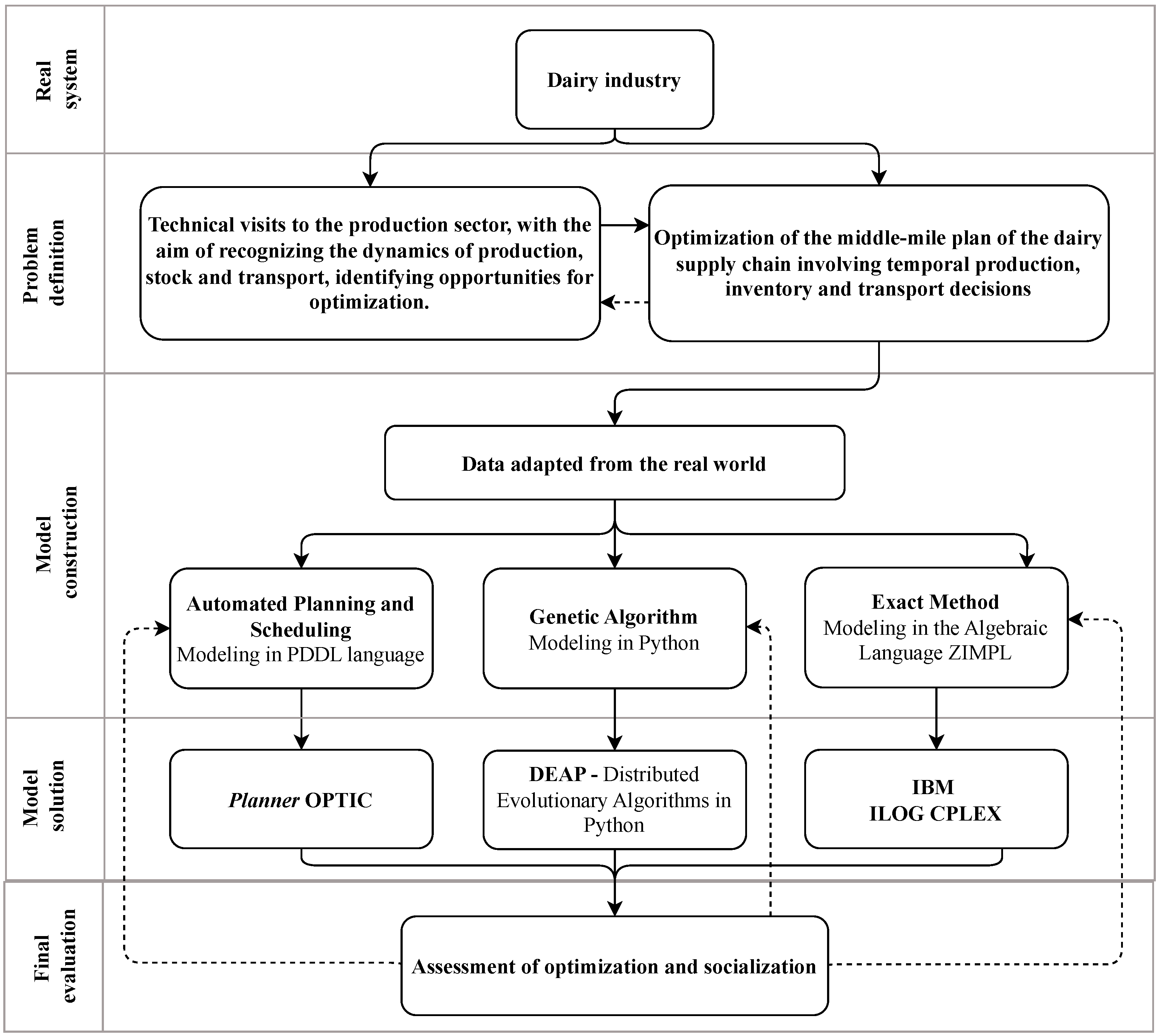
We developed three distinct models to address the problem, one formulated in PDDL (Planning Domain Definition Language), another implemented a Genetic Algorithm using the DEAP framework (Distributed Evolutionary Algorithms in Python), and a third based on MILP (Mixed-Integer Linear Programming). The solution strategies comprise Automated Planning and Scheduling (APS), solved by a temporal planner, applying a Genetic Algorithm, and resolving the MILP model through a commercial optimization solver, representing the exact method.

Another essential factor that is part of the scope of the problem is transportation, since there is a need to move products from one point to another. Many perishable materials and products are transported daily, and the limited shelf life of dairy products impacts operational and transport costs, environmental concerns, time constraints, stock relations, and high transporting frequency [7]. Transportation models related to the dairy industry have a distinct appeal from the point of view of supply chain logistics in general, and companies invest heavily in freight transport [21].

After understanding the dairy supply chain and its peculiarities in the issues of stretching and transport, this research applied optimization methods to the problem of inventory routing, coupled with the dairy production chain, with active production in 4 (four) processing plants, one distribution center, designating a mix of six products in a heterogenic fleet of 20 combustion vehicles and four electric forklifts. We developed a PDDL (Planning Domain Definition Language) and mathematical models to help solve the problem. The solving methods applied are Automated Planning and Scheduling, and we also implement a Genetic Algorithm and ran the mathematical model in a commercial solver.

The main objective is minimizing the makespan of the processes during the middle-mile stage, reducing the total time required to complete all operations. Consequently, this minimization affects product perishability, aiming to deliver products as early as possible, thereby reducing the risk of deterioration.

We intend to collaborate through this research to improve the milk supply chain by contributing to the academic evolution of research on perishable products, the dynamics of the dairy production chain, inventory management, and optimization methods with the support of artificial intelligence. This study fills an existing gap by examining middle-mile logistics, a less-explored area. It advances the state of the art by employing Automated Planning and Scheduling (APS) as an optimizer, comparing it with classical methods, an approach not previously explored in the literature.

After the introduction presented here, the structure of the article is the following: Section 2 presents the motivation of the study; Section 3 presents the description of the case study and the data used in the construction of the problem instance, such as factories, distribution centers, products, demand, production capacity, quarantine, transport and perishability; Section 4 describes the methodology adopted and the case study design; Section 5 presents the results obtained by the implemented methods; Section 6 analyses and discusses these results; and Section 7 presents the conclusions and future work. The appendices present some additional information.

2. Motivation

Due to the inherent perishability of its products, the dairy supply chain faces time-sensitive challenges, requiring strategies that optimize the production and distribution process to ensure products reach consumers as quickly as possible while maintaining commercial viability.

As pointed out in the introduction, previous studies highlight the importance of operational efficiency in this sector, yet a gap remains in the literature regarding the application of artificial intelligence to enhance middle-mile management in the stage between the production and distribution centers, which is a strong motivation for this study.

This paper supports this perspective by academically investigating a problem within a globally relevant market, aiming to benefit both theoretical and practical applications because milk and its derivatives are globally relevant commodities found worldwide. One of the main motivations is to study a real-life case to enhance practical applicability.

Given this scenario, this study explores and evaluates an AI tool to solve this challenge, aiming to reduce the makespan in the dairy production chain problem with a design based on the sector’s reality. This study adopts Automated Planning and Scheduling (APS) as the AI approach, recognizing it as a branch of artificial intelligence [22] that remains unexplored in this context. The use of APS for solving problems from industry is encouraged through in the context of the International Conference on Automated Planning and Scheduling [23]. APS performance is evaluated against classical methods, including the Genetic Algorithm (GA) and mathematical modeling based on Mixed-Integer Linear Programming (MILP), to identify the most promising approach for solving this problem.

The practical perspective of the presented problem considers real conditions and constraints observed in the dairy processing industry, aiming to make the implemented models tools of academic and practical interest for addressing issues related to the production, inventory, and logistics of dairy products.

In summary, the main contributions of this research are the following:

I. Proposal of a PDDL formulation for the Artificial Intelligence (Automated Planning and Scheduling) approach, integrating the features and constraints of the presented case study.

II. Proposition of a GA and MILP formulation as classical approaches.

III. Comparative analysis of the applied methods and identification of the best-performing approach for the studied problem.

IV. Academic contributions to a problem of global relevance.

3. Case Study: Dairy Industry

The case study contributes to investigations related to factual and present situations in daily life, with the opportunity to be evaluated and improved. Its main purpose is to analyze and solve problems in various fields. Despite being strongly related to social research, all areas use the case study method, whether associated with issues of the industrial or economic sector, since, regardless of the area of interest, the case study arises with the objective of understanding and investigating real-world situations in a more focused way [24].

The milk production chain has to address the question of the degree of perishable products very carefully, which can vary from days (milk in nature) to months (hard cheeses). A perishable product presents at least one of the following conditions: (1) its physical condition deteriorates visibly; (2) its internal or external value decreases in the customer’s perception; (3) the reduction in its functionality can lead to serious consequences [25].

The milk produced, respecting the appropriate conditions imposed by sanitary regulations, is stored in chillers on the properties or in community tanks. Trained professionals should perform its collection, performing several product quality tests before transporting it to the processing industries.

In Brazil, the person in charge of collection at the property measures the temperature, alkalinity, and acidity of milk [26]. If the milk passes the sanitary requirements, it is transported in isothermal tanks that cool the raw material in conditions suitable for processing. When arriving at the industrial plant, the raw material undergoes inspection, and again, tests are made to ensure that the milk has not undergone changes. In the processing industry, the raw material is stored properly at low temperatures to maintain its quality.

The dairy processing plant must coordinate the following three primary processes: (1) the transformation of raw materials into intermediate products, (2) the filling and packaging operations of final products, and (3) the transport of end products to distribution centers [27].

After the inspection approves the milk, it begins its transformation steps until each final product is produced. The dairy processing plants are segmented according to the final product to be produced. It is important to note that before any other process is performed, the milk is pasteurized. Depending on the production purpose, raw materials may suffer nutritional repairs of fat and protein, always from milk.

Each industry has peculiarities related to the organization of production and meeting demands. For example, some products can start production in one factory and end up in another, such as cheese that can be produced in one place and sliced in another. For the development of this research, interviews and technical visits were conducted in an important industry, with units in Brazil and around the world, aiming to understand the dynamics related to the production and transportation of dairy products.

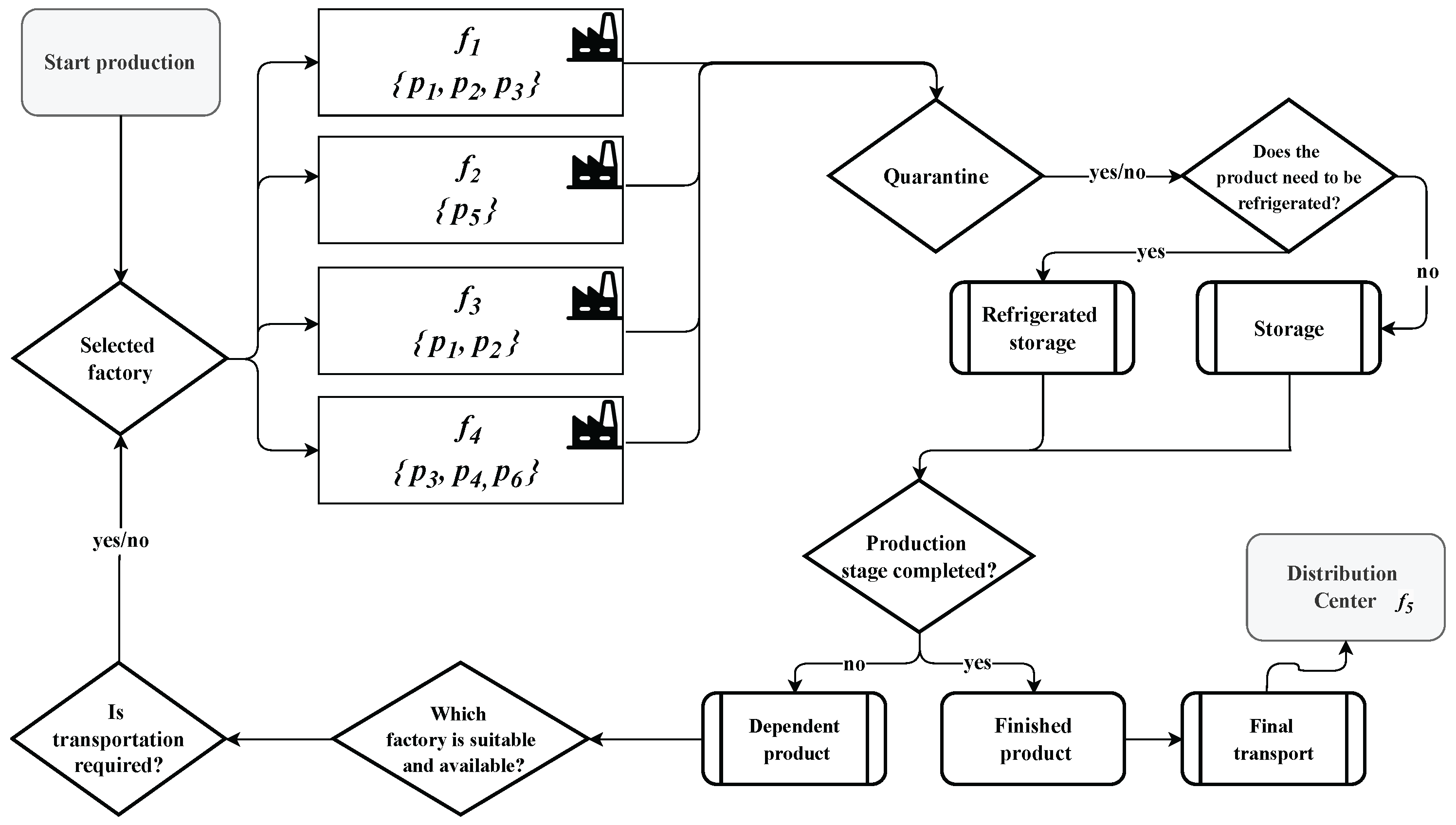
Figure 1 represents dairy products’ production, quarantine, and destination at the distribution center. After production is completed, products enter a quarantine period, except for dependent products. During this time, they remain in storage until released. Once released, dependent products undergo an additional processing stage at the original facility or another plant with available capacity. Final products released from quarantine are then transported to the distribution center. The objective of Figure 1 is to provide basic knowledge of the production dynamics of the entire milk chain since each derivative has a specific way of being produced.

The data used are adaptations of accurate information from the dairy production chain. The scope of the research concerns four dairy processing plants and one distribution center. We studied the behavior of six products as follows: four requiring refrigeration ($p_1$, $p_2$, $p_5$, $p_6$) and two dry ($p_3$, $p_4$). The problem seeks to meet all demands from the distribution center in the shortest time possible. The demands are monthly, allowing adjustments.

3.1. Dairy Plants

The case study relates to four geographically dispersed dairy plants ($F=\{f_1,\dots ,f_4\}$) and one distribution center (named $f_5$ for modeling’s sake, then $F^{\ast }=\{f_1,\dots ,f_5\}$).

The processing units have production capacity according to each product type, see

Table 1. Production characteristics.

P	${\mathit{TQ}}_{\mathit{p}}$	${\mathit{CF}}_{\mathit{f},\mathit{p}}$ (Tons)				$\mathit{I}{0}_{\mathit{f},\mathit{p}}$ (Tons)					${\mathit{DM}}_{\mathit{p}}$ (Tons)
		${\mathit{f}}_{\mathbf{1}}$	${\mathit{f}}_{\mathbf{2}}$	${\mathit{f}}_{\mathbf{3}}$	${\mathit{f}}_{\mathbf{4}}$	${\mathit{f}}_{\mathbf{1}}$	${\mathit{f}}_{\mathbf{2}}$	${\mathit{f}}_{\mathbf{3}}$	${\mathit{f}}_{\mathbf{4}}$	DC (${\mathit{f}}_{\mathbf{5}}$)	DC (${\mathit{f}}_{\mathbf{5}}$)
$p_1$	20	80.0000	-	80.0000	-	80.0000	-	80.0000	-	80.0000	420.0000
$p_2$	0	21.4200	-	21.4200	-	21.4200	-	21.4200	-	21.4200	200.0000
$p_3$	3	50.0000	-	-	50.0000	50.0000	-	-	50.0000	50.0000	300.0000
$p_4$	0	-	-	-	40.0000	-	-	-	40.0000	40.0000	200.0000
$p_5$	5	-	16.0000	-	-	-	16.0000	-	-	16.0000	130.0000
$p_6$	2	-	-	-	20.0000	-	-	-	20.0000	20.0000	380.0000

-: product p is not produced at factory f.

. There are six products produced ($p_1,\dots ,p_6$) by the four dairy plants; the relationship between products and plants is as follows:

–

$f_1$ produces $p_1$, $p_2$, and $p_3$.

–

$f_2$ produces $p_5$.

–

$f_3$ produces $p_1$ and $p_2$.

–

$f_4$ produces $p_3$, $p_4$, and $p_6$.

The dairy plants $f_1$, $f_3$, and $f_4$ can receive products from other units for completion; considering the entry of the unfinished product as input for a new one, they maintain the following relationships (see also

Table 2. Characteristics of products and factories.

F	Description	P	Packaging (kg)	Precedence	Lifespan
$f_1$	Cheese—piece	$p_1$	12.00	Input	180
$f_1$	Sliced cheese	$p_2$	0.15	Dependent on $p_1$	80
$f_1$	Milk powder—bag	$p_3$	25.00	Input	360
$f_2$	Brazilian cream cheese	$p_5$	0.20	Input	90
$f_3$	Cheese—piece	$p_1$	12.00	Input	180
$f_3$	Sliced cheese	$p_2$	0.15	Dependent on $p_1$	80
$f_4$	Milk powder—bag	$p_3$	25.00	Input	360
$f_4$	Milk powder—fractionated	$p_4$	0.20	Dependent on $p_3$	360
$f_4$	Butter	$p_6$	0.20	Input	150

):

–

$f_1$ can accept $p_1$ from $f_3$ and produces $p_2$.

–

$f_3$ can accept $p_1$ from $f_3$ and produces $p_2$.

–

$f_4$ can accept $p_3$ from $f_1$ and produces $p_4$.

–

All factories can send finished products to $f_5$ (distribution center). In this case study, we have only one distribution center (DC), also called $f_5$, for notation’s sake.

3.2. Distribution Center

The case study works with only one distribution center (DC), where all finished products are shipped. The distribution center is a factory f with a production capacity equal to zero and belongs to the set $F^{\ast }$, called $f_5$. As the planning horizon used in the case study is thirty days, we consider the storage capacity of $f_5$ unlimited for cold chamber storage and dry deposit storage.

3.3. Dairy Products

Dairy industries rely on diversifying dairy products and brands, which plays a key role in offering a wide range of nutritional options that meet multiple needs and preferences, meeting the growing demand for variety in consumers’ diets.

In this case study, the mix of dairy products involves products with distinct characteristics and different relationships between production plants to approximate the defined scope of the dairy industry context. Considering products with high demand, the diversity in quarantine times, the need for refrigerated storage or not, production precedence between products, products with the possibility of completion in more than one plant, and the need for refrigerated transport or not, the selected products are defined in the following set ($p_i\in P,i=1,\dots ,n_P$, where $n_P$ is the number of dairy products).

3.4. Dairy Product Demand

Production tries to meet the demand ($D{M}_{p_i}$) of each milk product ($p_i$) required in the distribution center ($f_5$). The planning horizon for meeting demand is monthly.

3.5. Production Capacity

The production capacities of the dairy plants are shown in Table 1, which refers to the production volume in tonnes that each factory can produce during one day of regular operation. Capacities do not limit the amount of resources needed for production and consider the installed infrastructure and efficiency of production processes.

We can also see in Table 1 the initial inventory of each product ($I{O}_{f,p}$) existing in each factory and the DC.

3.6. Quarantine Time

The quarantine of products in the food industry is a safety procedure used to isolate and temporarily retain food products. Only after this period can dairy products be released for further steps, such as transformation into a new product or transport to another industrial plant or distribution center.

Although strategies such as quarantine are not a requirement for perishable food processing industries, international standards recommend adopting measures focused on risk management, food safety, and minimizing risks to ensure compliance with regulations [28].

One of the main objectives of quarantine is to guarantee the quality of the product through additional tests, such as analysis, to detect microbiological, chemical, or physical contamination. It seeks to ensure food safety, minimize public health risks, and protect a brand’s reputation.

In this study, quarantine is mandatory after production in the first factory is completed, even if the product is shared and finished in another factory plant. For example, if factory $f_3$ produces product $p_2$ using product $p_1$ from factory $f_1$ as raw material, quarantine must take place obligatorily in $f_1$. From Table 1, it is possible to identify significant variations between each product’s quarantine times ($T{Q}_p$). The products $p_4$ and $p_5$ do not require quarantine because they have a precedence relation, i.e., the previous product has already passed through quarantine.

3.7. Transportation Time

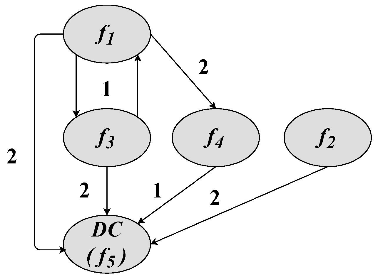
The cost of transportation is calculated in days, considering the total time required to complete the operation of moving products between the factories of origin and the destination ($T{T}_{f,f^{\prime }}$). We can observe those distances in Figure 2.

The transport time is calculated based on the kilometers traveled and converted into days.

3.8. Transportation Capacity

The transport of products between factories and even the distribution center $f_5$ is carried out through a heterogeneous fleet of vehicles with different capacities for dry or refrigerated cargo ($C{T}_{k,t}$).

Dry cargo vehicles transport various products with less stringent conservation requirements but are still subject to quality and safety standards. Refrigerated transport, or refrigeration, is essential for preserving perishable products sensitive to ambient temperature. Vehicles equipped with refrigeration systems prevent teh spoilage of food in transit. We consider the following four types of vehicles in the case study:

–

Type 1: Refrigerated van.

–

Type 2: Refrigerated truck.

–

Type 3: Dry cargo van.

–

Type 4: Electric forklifts.

Each factory, in each period, has a specific number of vehicles available for use, contracted to meet the demands; see

Table 3. Availability of vehicles per factory.

	Type 1			Type 2			Type 3	Type 4
	${\mathit{p}}_{\mathbf{1}}$	${\mathit{p}}_{\mathbf{2}}$	${\mathit{p}}_{\mathbf{5}}$	${\mathit{p}}_{\mathbf{1}}$	${\mathit{p}}_{\mathbf{2}}$	${\mathit{p}}_{\mathbf{5}}$	${\mathit{p}}_{\mathbf{3}}$	${\mathit{p}}_{\mathbf{3}}$	${\mathit{p}}_{\mathbf{4}}$	${\mathit{p}}_{\mathbf{6}}$
$C{T}_{k,t}$	21.1680	22.6800	17.2032	12.0960	12.9600	9.8304	25.0000	50.0000	50.0000	50.0000
Vehicles (${\mathcal{K}}_{f,t}$)	3		3	2		2	5	4
Factories	$f_1,f_3$	$f_1,f_3$	$f_2$	$f_1,f_3$	$f_1,f_3$	$f_2$	$f_1$	$f_4$	$f_4$	$f_4$

. The choice of vehicles respects the specificity of the transported product.

The vehicle is available for the factory when it is empty and not in transport. The vehicle is in use by the factory when it is attending to the operation of product transport, that is, a displacement between the origin factory (f) and the destination factory ($f^{\prime }$). As soon as the vehicle finishes its task, it is available at the factory of origin.

3.9. Perishability

One of the key consequences of makespan reduction in the case study is its impact on product perishability. Therefore, products should be placed in the distribution center as soon as possible. The shelf life of the products presented in Table 1 refers to the period during which each item maintains its quality and safety characteristics for consumption. Several factors influence products’ perishability, including hygiene manufacturing, adequate storage, and correct transport.

Therefore, with agile and appropriate planning, it is possible to guarantee the quality of the products. Thus, the product must be available in the distribution center before the demand meeting date, ensuring it is available for retail with a viable consumption life.

4. Case Study Design

Optimization problems are composed of inherent specificities and complexities. Thus, the adequacy of approaches based on sound theoretical principles provides support for the appropriate and necessary adaptation to solve these problems.

Basing the present research on the methodology of operational research, we adapted the phases of the study suggested by the authors of [29,30] to the case study of the dairy industry. Figure 3 demonstrates the methodological path adopted.

It is important to note that several technical visits and meetings with industrial plant employees were held to study the scope of the problem and understand the dynamics of the milk processing industry.

• Problem definition: The objective of the study is to optimize the dairy production chain, involving decisions on production, inventory, and transportation, taking into account perishability and environmental effects in the considered stages. The problem studied is limited to four dairy plants and one distribution center, whose production mix is processed in the factories and transported to the distribution center according to demand.
• Design and solution of the problem model: The challenge is to model the problem according to the industries’ characteristics, restrictions, and final goals. Through the data collected from the real problem, we present a mathematical model, which is the basis for the other computational models, as follows:

  –

  In the Automated Planning and Scheduling context, problem modeling occurs in files that define the domain and the problem. These files include the actions, preconditions, and effects that may occur, determining the rules and possible operations that the planner can perform. We use PDDL (Planning Domain Definition Language) as the language standard for modeling the problem, which is supported by the planner in this study [11,22,31,32]. The tuple $I,G,A$ defines the problem, generating plans that lead from the initial state $I$ to objectives $G$ through the application of sequence actions of $A$ [33,34]. The model will be optimized using Automated Planning and Scheduling, whose solver is a planner. We use OPTIC (Optimising Preferences and Time-Dependent Costs), an artificial intelligence planner that optimizes planning problems involving complex preferences and costs that vary with time [35].

  –

  We used the framework Distributed Evolutionary Algorithms in Python (DEAP 1.0) to model and solve the genetic algorithm [36].

  –

  We use the ZIMPL language to write the mathematical model [37]. ZIMPL allows the description of the MILP (mixed linear integer programming program) that represents the problem. This model will serve as an input for a commercial solver, in the case of IBM ILOG CPLEX Optimization Studio [38].

5. Computational Experiments

5.1. Mathematical Model

This subsection presents a single-objective model based on Mixed-Integer Linear Programming (MILP) to minimize the number of days required to satisfy total demand.

The mathematical model representing the problem aims to formally describe the elements involved, their constraints, and their objective.

Table 4. Mathematical model notation.

Index

d: time unit representing a single day within the planning horizon.

f: factory.

$f^{\prime }$: destination factory for the transport originating from factory f.

p: product.

$p^{\prime }$: product dependent on p as input.

t: vehicle type.

k: k-th vehicle of type t.

Sets

F: dairy milk plants ($f\in F=\{1,\dots ,n_F\}$).

$F^{\ast }$: extended dairy milk plants ($f\in F^{\ast }=\{1,\dots ,n_F\}$$\cup \left\{(n_F+1)\right\}$), where $(n_F+1)$ is the distribution center (DC).

${\mathcal{F}}_f$: destinations $f^{\prime }$ departing from plant f.

P: products ($p\in P=\{1,\dots ,n_P\}$).

${\mathcal{P}}_f$: products produced by plant f.

${\mathcal{P}}_p$: products $p^{\prime }$ produced from product p.

${\mathcal{T}}_f$: vehicle types available at the factory f.

${\mathcal{K}}_{f,t}$: vehicles type t available at the factory f.

D: time periods, in days ($d\in D=\{1,\dots ,n_d\}$).

Parameters

$n_F$: number of dairy plants.

$(n_F+1)orDC$: the distribution center.

$n_P$: number of products.

$T{Q}_p$: quarantine time of product p.

$T{T}_{f,f^{\prime }}$: transportation time between plant f and $f^{\prime }$.

$C{T}_{t,p}$: capacity of vehicle type t transporting product p.

$C{F}_{f,p}$: dairy plant f production capacity for product p.

$I{0}_{f,p}$: inital stock of product p at dairy plant f.

$D{M}_p$: product p demand.

Decision Variables

$I_{f,p,d}$: product stock p at dairy plant f on the day d.

$Q_{f,p,d}$: product stock p at dairy plant f released from quarantine on the day d.

$y_{f,p,d}$: quantity of product p produced on the day d in the dairy plant f.

${\widehat{y}}_{p^{\prime },f,p,d}$: quantity of the dependent product $p^{\prime }$ produced on the day d in the dairy plant f from the product p.

$x_{f,p,d,f^{\prime },t,k}$: quantity of product p transported from the dairy plant f to $f^{\prime }$ on the day d using the k-th vehicle of type t.

${\widehat{x}}_{f,p,d,f^{\prime },t,k}$: quantity of the product p received at the dairy plant $f^{\prime }$ from f on the day d using the k-th vehicle of type t.

$z_{f,p,d,f^{\prime },t,k}$: it assumes one (1) if the k-th type t is used to transport product p on the day d from dairy plant f to $f^{\prime }$; zero (0) otherwise.

$w_{p,d}$: it assumes one (1) if the demand for the product p is met on the day d; zero (0) otherwise.

$Tmax$: minimum number of days required to satisfy total demand.

presents the notation used by the mathematical model.

The model is formalized as follows.

$$\mathrm{Min}Tmax$$

(1)

$$\begin{array}{cc}\hfill & \hfill \\ \hfill & \mathbf{s}.\mathbf{a}\hfill \\ \hfill & I_{f,p,d}=I_{f,p,d-1}+Q_{f,p,d}+\hfill \\ \hfill & \sum _{f^{\prime }\in {\mathcal{F}}_f}\sum _{t\in {\mathcal{T}}_{f^{\prime }}}\sum _{k\in {\mathcal{K}}_{f^{\prime },t}}{\widehat{x}}_{f^{\prime },p,d,f,t,k}-\hfill \\ \hfill & \sum _{f^{\prime }\in {\mathcal{F}}_f}\sum _{k\in {\mathcal{K}}_f}{x}_{f,p,d,f^{\prime },k}-\sum _{p^{\prime }\in {\mathcal{P}}_p}{\widehat{y}}_{f,p,p^{\prime },d}\hfill & \hfill \forall f\in F,p\in {\mathcal{P}}_f,d\in D:d>0\end{array}$$

(2)

$$\begin{array}{ccc}\hfill & y_{f,p,d}=Q_{f,p,d+T{Q}_p+1}\hfill & \hfill \forall f\in F,p\in {\mathcal{P}}_f,d\in D\end{array}$$

(3)

$$\begin{array}{ccc}\hfill & {\widehat{y}}_{f,p,p^{\prime },d}=Q_{f,p^{\prime },d+T{Q}_{p^{\prime }}+1}\hfill & \hfill \forall f\in F,p\in P,p^{\prime }\in {\mathcal{P}}_p\cap {\mathcal{P}}_f,d\in D\end{array}$$

(4)

$$\begin{array}{ccc}\hfill & x_{f,p,d,f^{\prime },t,k}={\widehat{x}}_{f,p,d+T{T}_{f,f^{\prime }},f^{\prime },t,k}\hfill & \hfill \forall f\in F,p\in {\mathcal{P}}_f,d\in D,f^{\prime }\in {\mathcal{F}}_f,t\in {\mathcal{T}}_f,k\in {\mathcal{K}}_{f,t}\end{array}$$

(5)

$$\begin{array}{ccc}\hfill & x_{f,p,d,f^{\prime },t,k}\le C{T}_{t,p}{z}_{f,p,d,f^{\prime },t,k}\hfill & \hfill \forall f\in F,p\in {\mathcal{P}}_f,d\in D,f^{\prime }\in {\mathcal{F}}_f,t\in {\mathcal{T}}_f,k\in {\mathcal{K}}_{f,t}\end{array}$$

(6)

$$\begin{array}{c}{z}_{f,p,d,f^{\prime },t,k}+\hfill \\ \hfill \sum _{p^{\prime }\in {\mathcal{P}}_f}\sum _{\begin{array}{c}{d}^{\prime }\in D:\\ d<d^{\prime }\le d+T{T}_{f,f^{\prime }}\end{array}}\sum _{f^{\prime }\in {\mathcal{F}}_f}{z}_{f,p^{\prime },d^{\prime },f^{\prime },t,k}\le 1& \forall f\in F,p\in {\mathcal{P}}_f,d\in D,f^{\prime }\in {\mathcal{F}}_f,t\in {\mathcal{T}}_f,k\in {\mathcal{K}}_{f,t}\hfill \end{array}$$

(7)

$$\begin{array}{c}{I}_{DC,p,d}=I_{DC,p,d-1}+\hfill \\ \hfill \sum _{f\in F}\sum _{p\in {\mathcal{P}}_f}\sum _{t\in {\mathcal{T}}_f}\sum _{k\in {\mathcal{K}}_{f,t}}{\widehat{x}}_{f,p,d,DC,t,k}& \forall d\in D:d>0\hfill \end{array}$$

(8)

$$\begin{array}{ccc}\hfill & \sum _{d\in D}{w}_{p,d}=1\hfill & \hfill \forall p\in P\end{array}$$

(9)

$$\begin{array}{ccc}\hfill & I_{DC,p,d}\ge D{M}_p{w}_{p,d}\hfill & \hfill \forall p\in P,d\in D\end{array}$$

(10)

$$\begin{array}{ccc}\hfill & d{w}_{p,d}\le T_{\max }\hfill & \hfill \forall p\in P,d\in D\end{array}$$

(11)

$$\begin{array}{ccc}\hfill & I_{f,p,0}=I{0}_{f,p}\hfill & \hfill \forall f\in F^{\ast },p\in P\end{array}$$

(12)

$$\begin{array}{ccc}\hfill & I_{f,p,d}\ge 0\hfill & \hfill \forall f\in F^{\ast },p\in P,d\in D\end{array}$$

(13)

$$\begin{array}{ccc}\hfill & Q_{f,p,d}\ge 0\hfill & \hfill \forall f\in F,p\in {\mathcal{P}}_f,d\in D\end{array}$$

(14)

$$\begin{array}{ccc}\hfill & 0\le y_{f,p,d}\le C{F}_{f,p}\hfill & \hfill \forall f\in F,p\in {\mathcal{P}}_f,d\in D\end{array}$$

(15)

$$\begin{array}{ccc}\hfill & 0\le {\widehat{y}}_{p^{\prime },f,p,d}\le C{F}_{f,p}\hfill & \hfill \forall f\in F,p\in P,p^{\prime }\in {\mathcal{P}}_p\cap {\mathcal{P}}_f,d\in D\end{array}$$

(16)

$$\begin{array}{ccc}\hfill & x_{f,p,d,f^{\prime },t,k}\ge 0\hfill & \hfill \forall f\in F,p\in {\mathcal{P}}_f,d\in D,f^{\prime }\in {\mathcal{F}}_f,t\in {\mathcal{T}}_f,k\in {\mathcal{K}}_{f,t}\end{array}$$

(17)

$$\begin{array}{ccc}\hfill & {\widehat{x}}_{f,p,d,f^{\prime },t,k}\ge 0\hfill & \hfill \forall f\in F,p\in {\mathcal{P}}_f,d\in D,f^{\prime }\in {\mathcal{F}}_f,t\in {\mathcal{T}}_f,k\in {\mathcal{K}}_{f,t}\end{array}$$

(18)

$$\begin{array}{ccc}\hfill & z_{f,p,d,f^{\prime },t,k}\in \{0,1\}\hfill & \hfill \forall f\in F,p\in P,d\in D,f^{\prime }\in {\mathcal{F}}_f,t\in {\mathcal{T}}_f,k\in {\mathcal{K}}_{f,t}\end{array}$$

(19)

$$\begin{array}{ccc}\hfill & w_{p,d}\in \{0,1\}\hfill & \hfill \forall p\in P,d\in D\end{array}$$

(20)

$$\begin{array}{ccc}\hfill & Tmax\ge 0\hfill & \hfill \forall d\in D\end{array}$$

(21)

The objective, represented in Equation (1), is to minimize the total execution time of a demand response plan at the distribution center.

Equation (2) represents the stock conservation constraints, where the first part represents the sum of the previous day’s production, the stock of products available after quarantine, and the products arriving from other factories. The second part of Equation (2) represents the decrease in stock, subtracting the products that are sent to other factories and also subtracting the stock benefited in dependent productions, reducing the amount of product input. Equations (3) and (4) define the quantity of products released for transport to the distribution center or benefiting in another dairy plant on the day after the end of quarantine. Equation (4) refers to the production of a product that depends on previous production.

Equation (5) indicates that the quantity of product transported between factories must be equal to the quantity arriving at the factory destination after the transportation time. Equation (6) indicates that the load carried in the selected vehicle must not exceed its maximum capacity.

Equation (7) imposes a constraint that ensures the k-th vehicle of type t is assigned to only one transit operation between an origin factory f and a destination factory $f^{\prime }$ within the defined period. This restriction prevents a vehicle from being used in multiple transits concurrently. The formulation accounts for all product flows from factory f, represented by the summation over $p^{\prime }\in P_f$. Additionally, the summation over $d^{\prime }\in D$ considers the feasible arrival days, ensuring that any vehicle arriving at $f^{\prime }$ on day $d^{\prime }$ must have departed earlier, respecting the required travel time $T{T}_{f,f^{\prime }}$. During this interval, the vehicle remains in transit and cannot be allocated to any other trip, preventing scheduling conflicts. The summation over $f^{\prime }\in F_f$ includes all potential destination factories that receive products from f.

Equation (8) updates the stock in the CD, and the demand response constraint is Equation (10). Equation (9) determines that all products will have their demands satisfied sometime within the planning horizon, guaranteeing a feasible solution. Equations (10) and (11) define the value of $Tmax$. Equation (10) determines when each product meets its demand, and Equation (11) indicates when all products meet the demand, i.e., the maximum amount of time to satisfy the demand. Equation (12) defines each factory’s initial stock.

Equations (13)–(21) define the variables’ domain. Equations (15) and (16) represent the capacity constraints in the model, establishing the relationship between production variables and factory capacity. These equations ensure that the quantity of manufactured products does not exceed production capacity, which, in turn, implicitly limits the supply to the DC, reflecting the real constraints of the supply chain.

The variables expressed in Equations (19) and (20) are binary, representing discrete decisions related to vehicle allocation for transportation and demand fulfillment on a given day. The variable $Tmax$ is defined within the domain of non-negative real numbers, as established by constraint (21). However, since the objective function is formulated as a minimization problem and in conjunction with constraint (11), $T_{max}$ assumes only integer values in the optimal solution. The remaining variables (see Equations (13), (14), (17), and (18)) are continuous because demand is expressed in tons, with a precision of up to four decimal places, ensuring an accurate approximation in the modeling of production, inventory, and transportation.

5.2. Automated Planning and Scheduling (APS)

The characterization of Automated Planning and Scheduling makes use of the following three parts: (1) models—composed of the structure of the domain, actions, objective, and initial state; (2) language—the chosen way to express the model to be understood by the planner, is the language PDDL; (3) planner—the algorithmic search strategy for navigating and optimizing the model [39]. The modeling of APS problems occurs in domain and problem files.

The actions define the rules that govern the behavior of objects; they are related to the changes in state that may occur in the modeled problem. The action modeling indicates how the environment can change from one state to another, and the goal is to find a sequence of actions that leads from an initial state to the state of the goal or objective state. In the problem file, the initial state defines the available resources and conditions necessary to start the plan, whose goal state formalizes the objectives.

The file with the domain description defines the rules governing the behavior of objects, while the problem file defines the addressed problem, including the initial conditions and objectives.

OPTIC was the planner solver for resolving the model, aiming to minimize the makespan [35]. Time planning deals with actions related to time. Those actions can also occur simultaneously, and the duration of actions may vary. Actions may also have complex interdependencies that determine what combinations are possible [39].

The OPTIC planner uses the Simple Temporal Network (STN) and the Single-Source Shortest Path (SSSP) algorithm to adjust the objective function and ensure the fulfillment of cost functions in time. It employs the following admissible heuristics: one based on plan relaxation, which simplifies the search while maintaining feasibility; and another to eliminate unfeasible branches, refining the solution. The tree search starts with the high cost of quickly discarding suboptimal paths, gradually reducing it with additional cuts. For its execution, it is necessary to install a solver, such as Coin-or Linear Programming (CLP).

The goal is to find a sequence of actions that transforms the initial state into the desired goal state. The tuple used is as follows:

(a)

Initial state (I)

–

Demand: Demand f of each dairy product $D{M}_p$.

–

Dairy Plants: The factories producing each product $P_f$ and daily production limits $C{F}_{f,p}$.

–

Quarantine Time: Quarantine time for each product $T{Q}_p$.

–

Initial Stock: Stock, in tons, of each product at each factory $I{0}_{f,p}$ when optimization starts.

–

Vehicles: Vehicles that are available at each factory for transport ${\mathcal{K}}_f$, respecting the transport capacity $C{K}_{k,p}$. Furthermore, this informs the possible routes that each vehicle can travel ${\mathcal{F}}_f$.

–

Distances: The distance between source and destination dairy plants, measured in days $T{T}_{f,f^{\prime }}$.

(b)

Goal state (G):

–

Demand fulfillment: The goal state of the model seeks that the DC meets the demand for all products. It means that the available stocks of each product in the distribution center are equal to or greater than the respective demands $I_{DC,p,d}\ge D{M}_p$.

(c)

Action (A):

–

Produce: The production quantity of each product produced in a dairy plant (respecting its capacity) will increase the quarantine stock or the available stock if the product does not require quarantine. The duration of this action is set to one time unit (one day).

–

Sharing: This allows a product released from quarantine to be transported to a factory that will transform this input into a derivative product, as is the case of $p_2$ and $p_4$ production, which need p1 and p3, respectively, (see Section 3.1). The action increases the destination factory’s available stock.

–

Quarantine: The quarantine stock receives finished products and respects each product’s quarantine time. At the end of the quarantine action, it moves the products to the available stock so that other actions, such as transportation, occur.

–

Send: The send action represents the transport of products between factories and between factories and the DC. This action considers the availability of vehicles and the distance in days between origin and destination. The effect of this action is the increase of products in the destination factory and the subtraction of the stock in the origin factory.

(d)

Metrics: The objective of the model is to minimize a function that considers the total cost associated with production, transportation, and storage time. Thus, the APS aims to find a solution that satisfies the conditions of the goal state, seeking to minimize the makespan.

5.3. Plan Found by OPTIC

Executing the OPTIC planner for the problem modeled in PDDL generates a complete solution plan, whose steps in finding the best possible solution are documented and available in the GitHub repository (see Section 6.2).

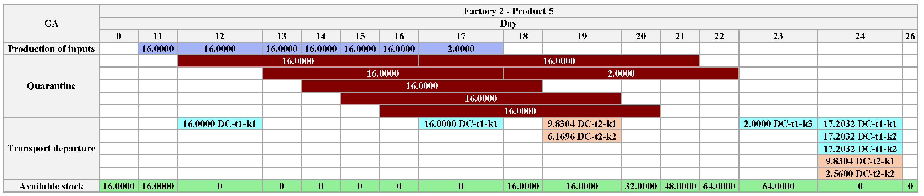
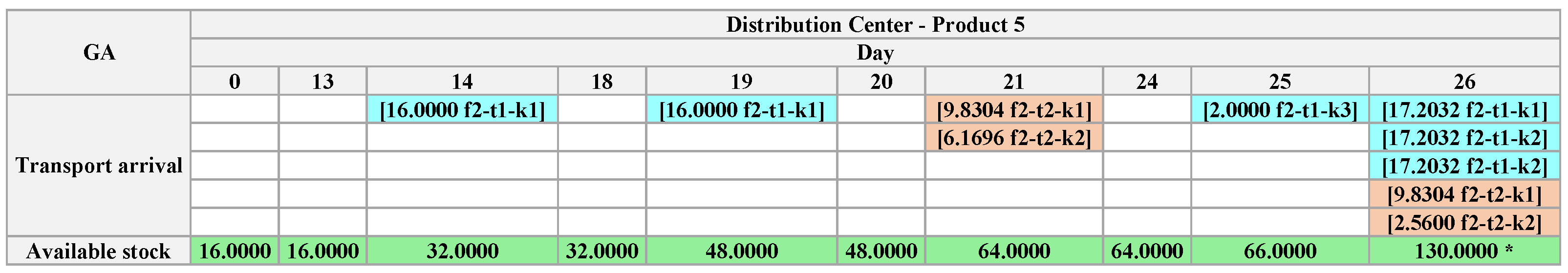
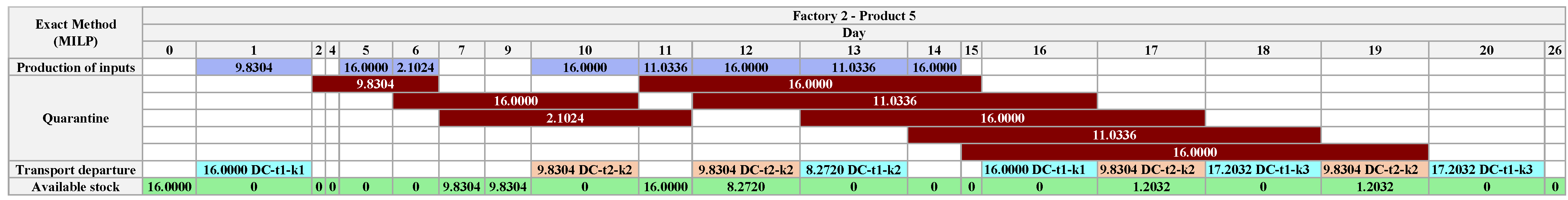
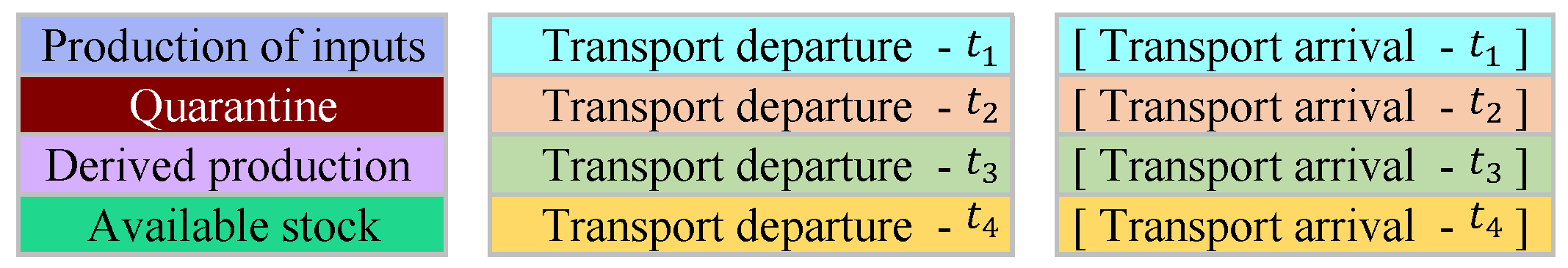
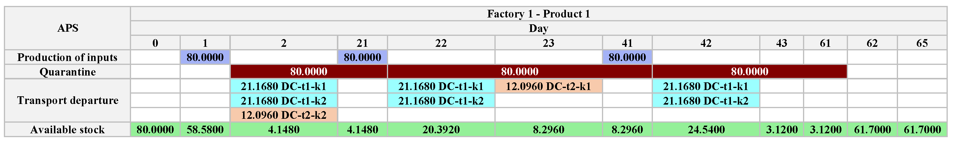
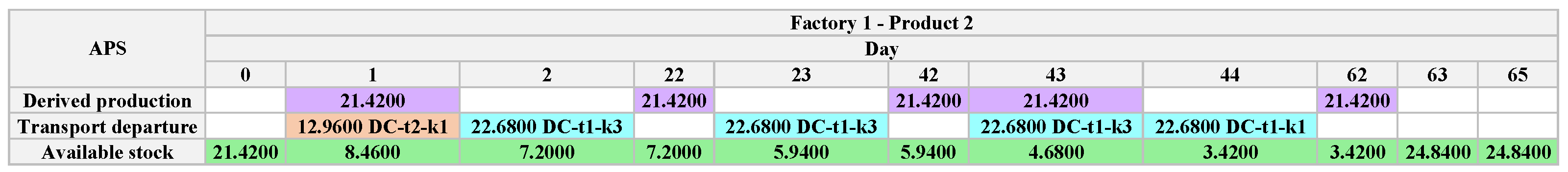
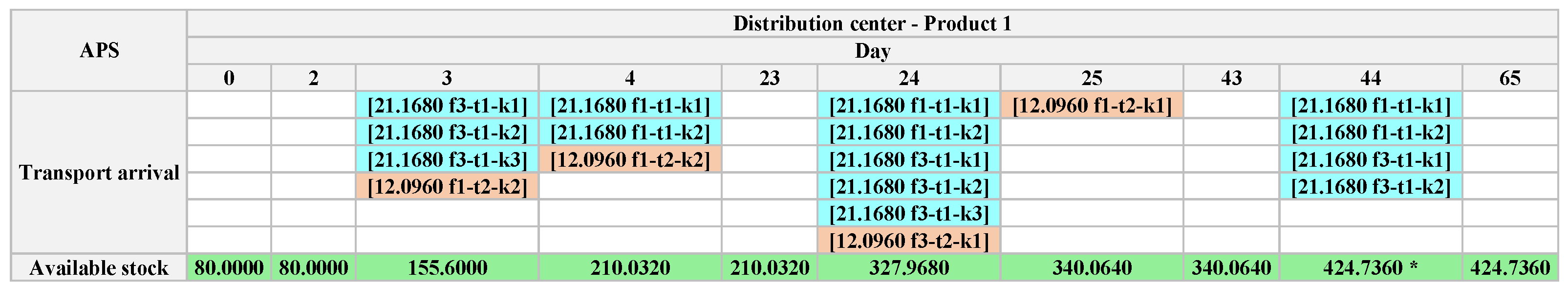
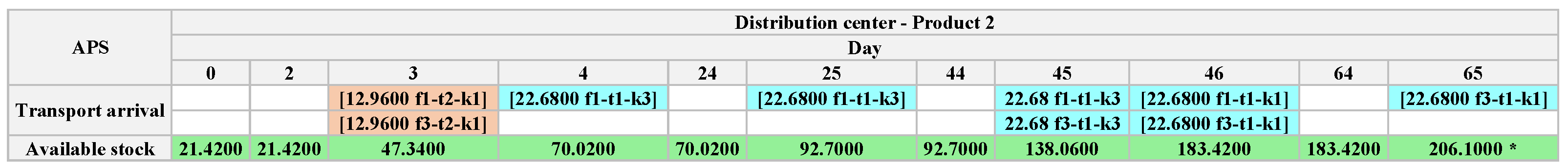
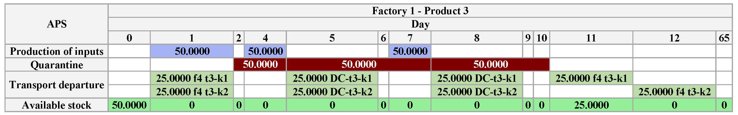
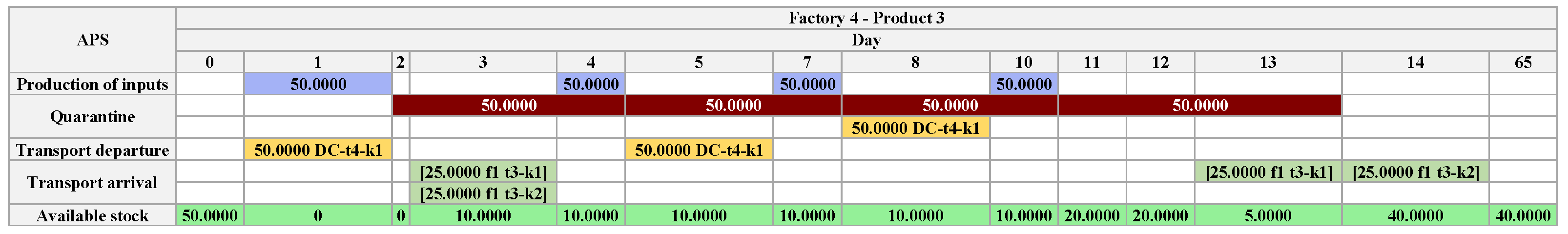
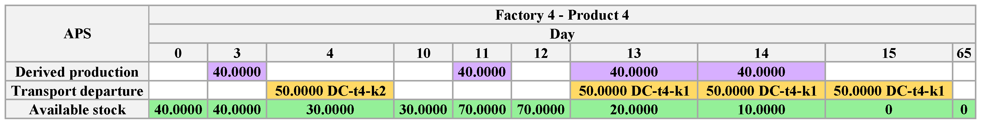
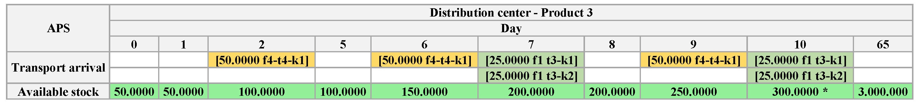
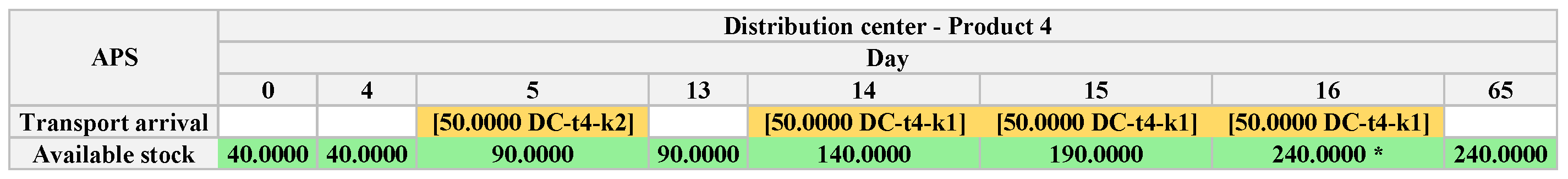
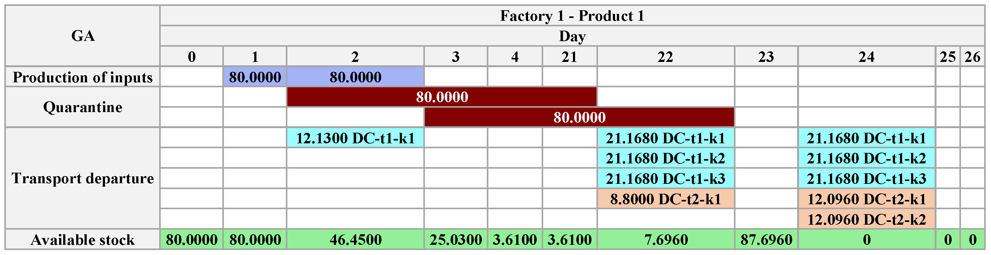
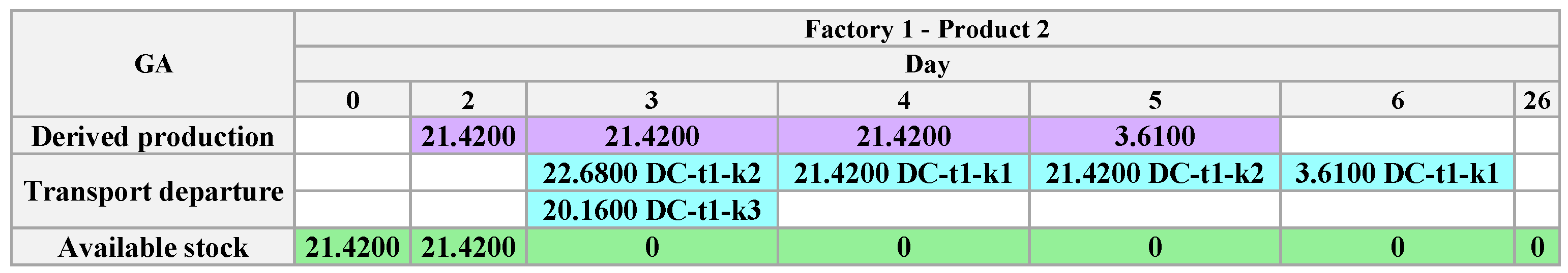
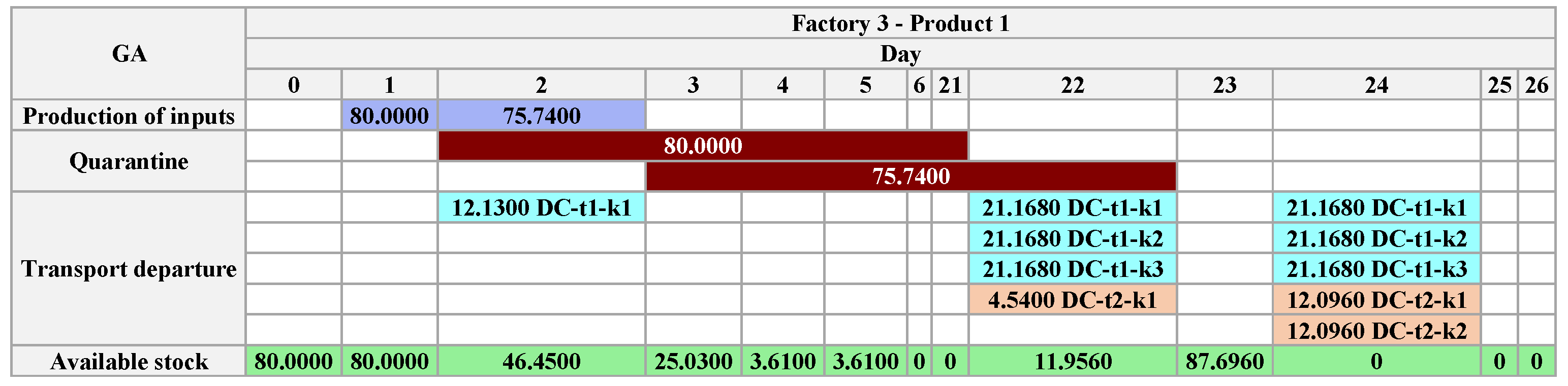
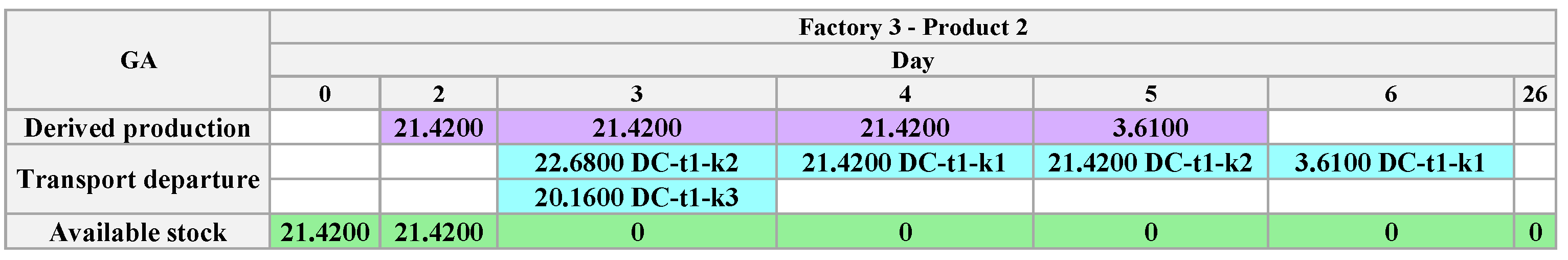
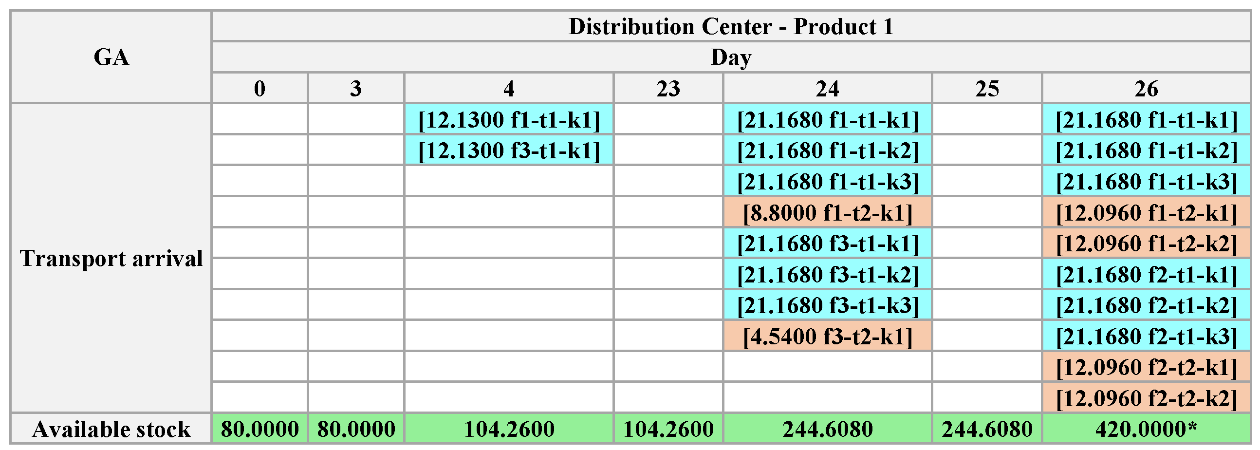
The solution obtained through the methods used to solve the problem is graphically displayed in a unified structure over the time horizon. Figure 4 shows the legend used in the graph, which depicts the actions that occur during the production process. The activities depicted include production, quarantining, transportation, and demand fulfillment (at the DC). The representation excludes days when there was no relevant activity observed.

The color scheme of Figure 4 represents different stages of the supply chain as follows: blue indicates input production, dark red represents the quarantine period, purple corresponds to derived production, and green signifies available stock. In transportation, the color varies according to the vehicle type (t), as follows: light blue for $t_1$, light orange for $t_2$, light green for $t_3$, and yellow for $t_4$. The arrival transport at the destination factory ($f^{\prime }$) follows the same color scheme but is enclosed in [ ] to distinguish it from departure transport.

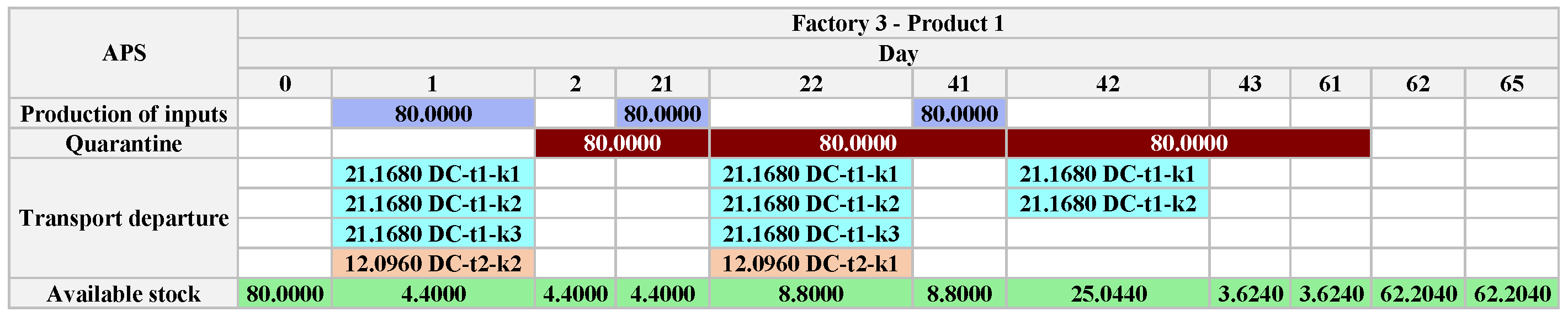
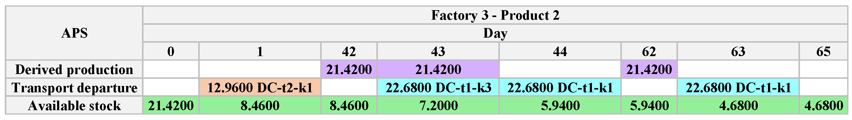
Figure 5, Figure 6, Figure 7, Figure 8, Figure 9, Figure 10, Figure 11, Figure 12, Figure 13, Figure 14, Figure 15, Figure 16, Figure 17, Figure 18 and Figure 19 show the activities of the solution found by APS for this case study.

We can observe that the solution proposed by APS starts production on the last day of quarantine of a previous production. As a consequence of this decision, there may be a delay in meeting the demand for inputs and/or dependent products.

When a product is released from quarantine stock, the solution process aims to use it immediately for dependent production or transportation. However, as in production, transportation is always carried out with the maximum capacity, leaving in stock the quantity that cannot be transported or used as an input for a dependent product.

We observed that the production of $p_1$ starts on $d_1$ in both $f_1$ and $f_3$ (see Figure 5 and Figure 7). From the initial stock of $p_1$ in $f_1$, 21.4200 tons are sliced on $d_1$ (producing $p_2$), while 54.4320 are sent to the DC on $d_2$ (see Figure 5 and Figure 6).

In $f_3$, almost all the initial stock of $p_1$ is transported to the DC on $d_1$, as well the stock available at $d_{22}$, causing $p_2$ production to start only on $d_{42}$ and delaying all production planning (see Figure 7 and Figure 8).

Due to $p_2$’s dependence on $p_1$ production and APS’s prioritization of first meeting all demands for $p_1$ (which happens on $d_{44}$), the satisfaction of the demand for $p_2$ only occurs on $d_{65}$, quite far from the desired horizon of 30 days (see Figure 9 and Figure 10).

For $p_3$ and $p_4$, demand is met within the planning horizon, $d_{10}$ and $d_{16}$, respectively, (see Figure 7, Figure 8, Figure 9, Figure 10, Figure 11, Figure 12, Figure 13, Figure 14 and Figure 15). The APS trend to meet demand remains, but as the quarantine period is shorter, the demand service takes place within the planning horizon. However, for products $p_5$ and $p_6$, the demands were not satisfied within the planning horizon, occurring only on $d_{38}$ and $d_{47}$, respectively (see Figure 16, Figure 17, Figure 18 and Figure 19).

We observed that APS has difficulties efficiently organizing production and using transport vehicles. These difficulties are inherent to a MILP like this, so we will see how the problem is solved using the CPLEX solver (Exact Method) and the GA.

After the execution of the APS model, the system found a production plan but did not find a plan solution that was considered optimal. A critical point identified was the absence of production during the period in which the quarantine action was taking place. Nothing in the modeling restricts actions to co-occur with the quarantine period. This situation resulted in the underutilization of factories on the 30-day planning horizon, compromising the productive flow and efficiency of actions and impacting the non-fulfillment of demand.

The state of the goal (b) requires that $I_{DC,p,d}\ge D{M}_p$. Due to this, the production was interrupted only when we it fulfilled the demand in $DC$, which resulted in the generation of stocks in the factories already producing.

Table 5. Product stock remaining in dairy plants, in tons.

P	${\mathit{f}}_1$		${\mathit{f}}_2$		${\mathit{f}}_3$		${\mathit{f}}_4$		DC (${\mathit{f}}_5$)
	Stock	$\mathit{d}$		$\mathit{d}$	Stock	$\mathit{d}$	Stock	$\mathit{d}$	Stock	$\mathit{d}$
$p_1$	61.7000	62	-	-	62.2040	62	-	-	424.7360	44
$p_2$	24.8400	63	-	-	4.6800	63	-	-	206.1000	65
$p_3$	0	12	-	-	-	-	40.0000	14	300.0000	10
$p_4$	-	-	-	-	-	-	0	15	240.0000	16
$p_5$	-	-	5.1200	37	-	-	-	-	138.8800	39
$p_6$	-	-	-	-	-	-	0	40	420.0000	41

shows the quantity of each product, in tons, that remains stored in the factories. An example of the planner’s wrong decisions is that the demand for $p_1$ is satisfied on $d_{44}$. However, as $p_2$ needs $p_1$, the production of $p_1$ continues until it supplies the demand for $p_2$, generating unnecessary stock.

Note that the production plan of OPTIC needs 65 days to satisfy all the demands in the $DC$; in the following sections, we will see that this is more than twice the solutions obtained by the other methods. All files related to the modeling and execution of the planner are available on GitHub; see Section 6.2.

5.4. Genetic Algorithm (GA)

The development of Genetic Algorithm (GA) code uses the DEAP (Distributed Evolutionary Algorithms in Python) library, which provides a robust and flexible framework for implementing evolutionary algorithms for optimization problems.

The GA modeling was adapted to the problem studied, respecting all the conditions and restrictions previously presented.

5.4.1. GA Pseudocode

To better understand the GA, we present the additional notation in

Table 6. GA additional notation.

GA Additional Notation
$PGA$: population in Genetic Algorithm.
i: initial individuals.
j: next generation individuals.
$G_{d,p,DC}$: this gene corresponds to the date of the initial production for product p.
$G_{d,p,DC}^{\prime }$: this gene corresponds to the date of the final transport arrival required to meet the demand for product p.

together with the corresponding pseudocode (see Algorithm 1).

Algorithm 1 GA for the case study in dairy plants

1: Input: demands $D{M}_p$, initial stocks $I{0}_{f,p}$, production capacities of each dairy plant $C{F}_{f,p}$, vehicle capacities $C{K}_{k,p}$, quarantine times $T{Q}_p$ and stocks in the distribution center $I_{DC,p,d}$.   2: Initialize $PGA$ with random individuals representing the delivery days for each product.   3: while (number of generations ≤ 20) do   4:       for (each individual i in $PGA$) do   5:             Calculate production, quarantine and transport phases of i using the function ‘calculate_phases’.   6:             Assess the feasibility of i using the function ‘is_feasible’, applying penalties if necessary.   7:             Compute $Tmax$ of i considering the time to fulfill the demand at DC.   8:       end for   9:       Select the individuals for crossover. 10:       Apply Two-point crossover in 80% of selected individuals. 11:       Apply mutation in the individuals of the new population with a probability of 30%. 12:       for (each individual j of new population) do 13:             Reevaluate phases of j with function ‘calculate_phases’ 14:             Check and correct precedence between products with ‘repair_individual’ 15:             Evaluate j. 16:       end for 17:       Update population. 18: end while 19: Identify the individual with the lowest $Tmax$ (best fitness) between generations. 20: Output: best individual.

5.4.2. Example of GA Individual and Operators

Below is an example of the operations performed on the individuals generated for this problem, as follows:

(a)

Individual: Each individual is randomly generated, with each gene representing the total delivery time for a product at the Distribution Center (DC), within a time window ranging from 1 to 30 days. For example, individual1 = [5, 2, 15, 20, 13, 7] indicates that the total delivery time for the first product is scheduled for day 5, the second product on day 2, and so on. The size of the vector corresponds to the number of products (six products in this case). Similarly, individual2 = [6, 12, 14, 18, 9, 21] represents another set of delivery days for the same products.

(b)

Crossover: We use the two-point crossover operator to combine two individuals and generate two new individuals. This operation exchanges segments between the two parents, creating hybrid offspring.

Example:

• offspring1 = [5, 2, 14, 18, 13, 17]
  offspring2 = [6, 12, 15, 20, 9, 21]

(c)

Mutation: Mutation uses the mutFlipBit operator, which randomly changes the delivery date of products on the DC with a probability of 30%. This operation introduces variations, exploring different solutions in the search space.

Example:

• offspring1_after_mutation = [7, 2 14, 18, 13, 17]

(d)

Repair: The repairing function ensures that individuals respect all the constraints, rules of precedence, and dependence between products.

Example:

• offspring1_after_repair = [7, 8, 14, 18, 13, 17]

(e)

Selection: We employ the elitism method, where the best individuals from the current population are retained for the next generation without modification. The Hall of Fame (hof) structure is used to store these individuals, ensuring that the best solutions found across generations are preserved.

(f)

Fitness: The objective function seeks to minimize the maximum time of service of all demand in the DC ($Tmax$). Therefore, the best individual is the one with the lowest value of $Tmax$.

Example:

• offspring1 = [5, 2, 14, 18, 13, 7] $\to T_{max}$ = 60 (Given that this individual is infeasible and requires correction.)
  offspring1_after_repair = [7, 8, 14, 18, 13, 17] $\to T_{max}$ = 18
  offspring2 = [6, 12, 14, 18, 9, 21] $\to T_{max}$ = 21

In the example above, each gene is evaluated based on the total time required to deliver the product, considering production, quarantine, and transportation times. In the case of offspring1, the delivery time of the second product, which is 2, was considered infeasible, resulting in a penalty of 60. On the other hand, offspring1_after_repair, after being corrected, obtained a $Tmax$ of 18 and was selected as the best individual for the next generation.

(g)

Population: The population size is 50 individuals. The initial population is made up of randomly generated individuals, with each individual representing a solution to the production and transportation scheduling problem. The evolution of the population occurs through crossover and mutation operations, creating new solutions and selecting the best ones to form the next generations

(h)

Stopping Criteria: The GA ran for 20 generations, each composed of a new population of individuals generated by crossover and mutation. The objective was to minimize $Tmax$ and ensure that all products were delivered in the DC in the shortest possible time.

5.4.3. Individual Coding and Decoding

• First phase—individual coding:

The coding of each individual begins with the definition of the value of each gene, where its locus represents the product and its value represents the day on which the product meets the demand in the $DC\left(G_{d,p,DC}^{\prime }\right)$. The value of each gene is randomly selected in the interval between $d_1$ and $d_{30}$, which corresponds to the planning horizon.

From the definition of the value of the genes, we start to calculate the day of production of each product. The productions are triggered according to the demand of each product ($D{M}_p$), and its production time is taken into account. The initial stocks of each product in the factories ($I_{f,p,d}$) and $DC$ are also considered, along with the production capacity of the factories ($C{F}_{f,p}$), production time, quarantine time ($T{Q}_p$), and time required for transport. The transport time considers the transport capacity ($C{T}_p$) and transportation cost between the origin factory f and destination factory $f^{\prime }$. With this information, we can find out how many days we should return to meet all products’ demands.

When the products are dependent ${\mathcal{P}}_p$, the calculation should consider both the demand of the dependent product and its source.

If the production exceeds the transport capacity $C{T}_{t,p}$, the transport time will be adjusted to double the standard value $T{T}_{p,f,f^{\prime }}$; otherwise, we use the standard value.

The solution should be repaired if the production start date is less than $d_1$. Repair is performed by randomly choosing a new date between the current value of the gene and $d_{30}$. The coding process establishes the necessary parameters for the execution of the production and transport function in the genetic algorithm model, preparing the individual to be evaluated in the following phases of the algorithm.

Example: If the gene corresponding to $p_1$ receives the value 26 and considering 2 days of production, 20 days of quarantine, and 4 days of transport, the beginning of production of $p_1$ is computed as follows:

$$\begin{array}{cc}\hfill G_{d,1,DC}& =\mathbf{26}-2-20-4+1=1\hfill \end{array}$$

(22)

Thus, the production of $p_1$ will start on $d_1$. With the determination of the dates of the beginning and end of production, the dates of beginning and end of quarantine, as well as the beginning and end of transport are defined in sequence, observing the criteria of precedence between products, the stocks available in the factories and the total transport capacity. Notice that these phases are the time windows in which each process begins and ends; however, a detailed description of the solution is not presented at this stage.

In the next step, the generated individuals undergo crossing and mutation operations, generating their offspring. Then, for each gene, it is verified if the beginning of the resulting production is negative, which would indicate the unfeasibility of the delivery date. If this occurs, a repair procedure is applied in which a new number is generated randomly in the range from 1 to 30. If, even after the repair, some gene remains unviable, the solution receives a penalty of 60.

• Second phase—individual decoding:

Knowing the start of production and transportation dates for each product, the production of each product begins in its respective factories. Then, the product is quarantined, at the end of which the production plan can use it to produce a dependent product or send it to the DC.

The transport respects the constraints on the use of vehicles and their capacities. Then, we adjust the delivery dates of each product in DC. The incumbent solution is updated, and a new cycle begins until the stop criterion is satisfied.

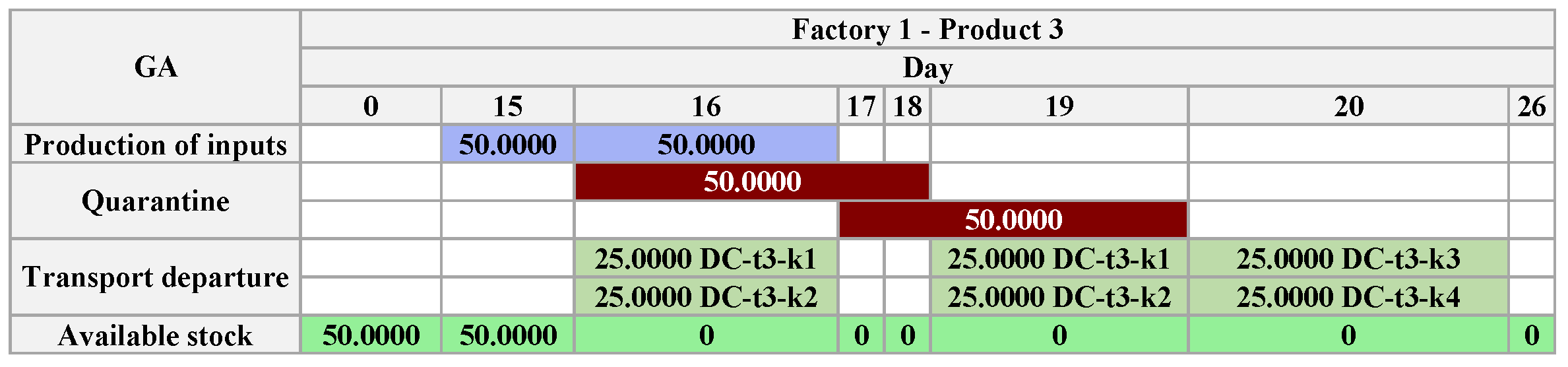
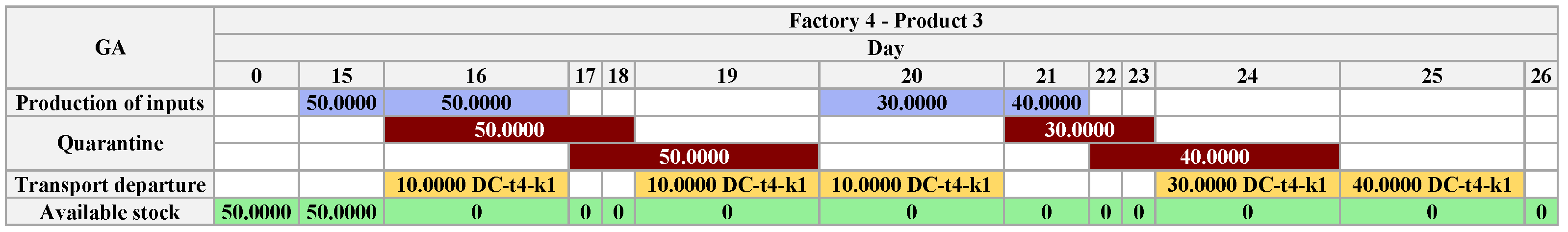
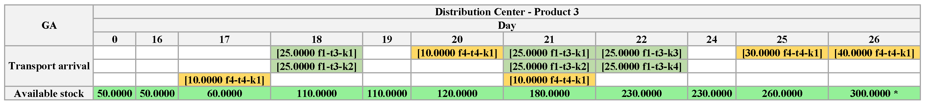
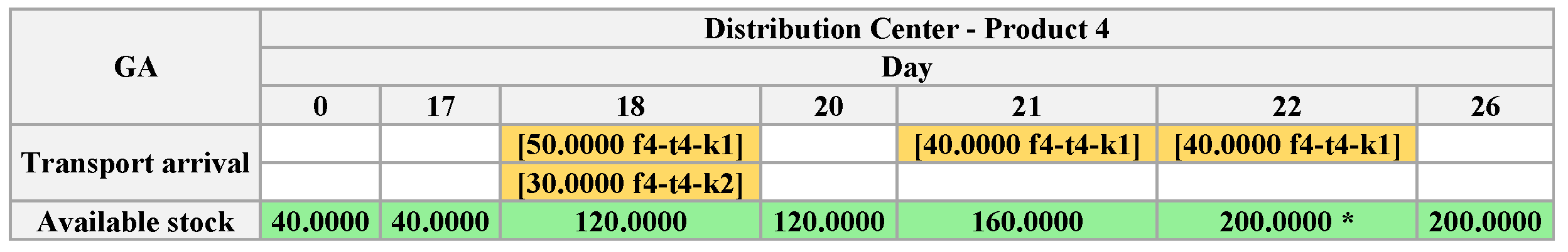
5.4.4. Plan Found by GA

The GA found a solution that meets all demand in the DC in 26 days, a reduction of 60% compared to APS. The figures follow the pattern from APS, using the same legend shown in Figure 4.

According to the representation of the solution, exposed between Figure 20, Figure 21, Figure 22, Figure 23, Figure 24 and Figure 25 (representing $p_1$ and $p_2$, in factories $f_1$ and $f_3$ and the $DC$), the rest of the production plan is in Appendix A.1. We show $f_1$ and $f_3$ and the $DC$ are sufficient, as the total production time depends on them. We observed that the GA solution reduces factory inventories, allocating available production to transport processes or dependent output.

As shown in Figure 21, Figure 23, and Figure 25 and Appendix A.1, the GA seeks to meet the demand of dependent products $p_2$ and $p_4$. In contrast, the input products $p_1$ and $p_3$ are served later, as shown in Figure 20, Figure 22, and Figure 24 and Appendix A.1.

Unlike the APS and the Exact Method, in the GA, there is no transport between producing factories; the products are sent directly to the $DC$. Thus, the product $p_3$ produced in $f_1$ is sent directly to the DC, $p_3$ produced in $f_4$ is input to produce $p_4$, and the remaining stock is sent to the $DC$. The transport allowed between factories $f_1$ and $f_3$ also does not occur. Finally, the mandatory product in the optimization process of the GA is $p_1$, which determines the $Tmax$, finishing $d_{26}$.

5.5. Exact Method

For the solution of the mathematical model presented in Section 5.1, we used the solver IBM ILOG CPLEX. CPLEX found the optimal solution to the proposed problem, respecting the capacity and processing time constraints. All factories start with the stock available according to Table 1.

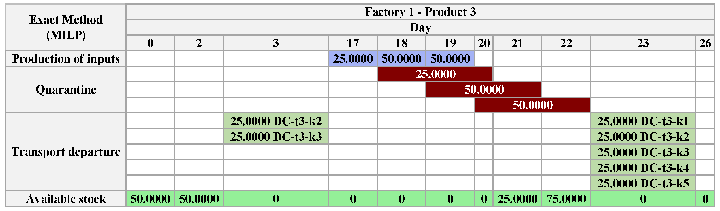
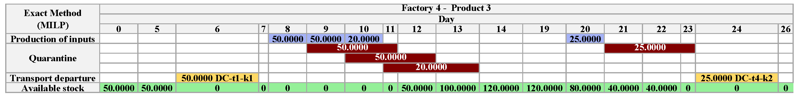
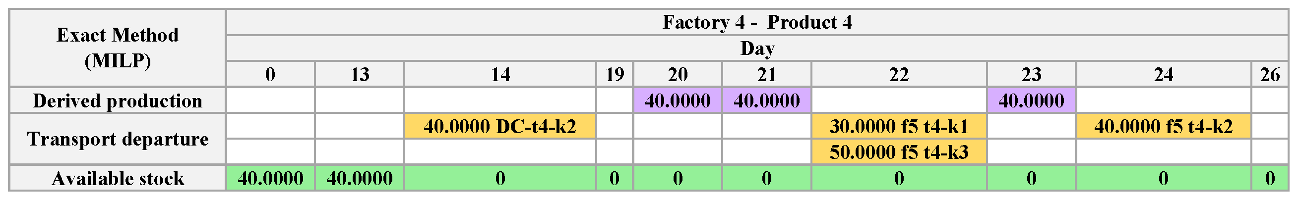
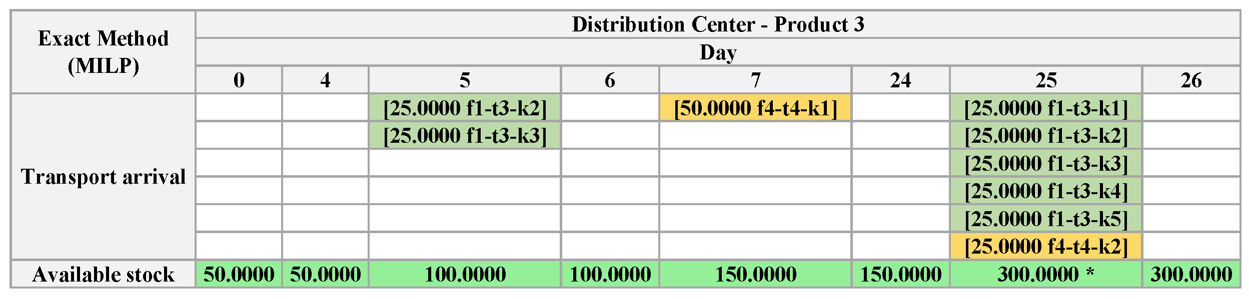
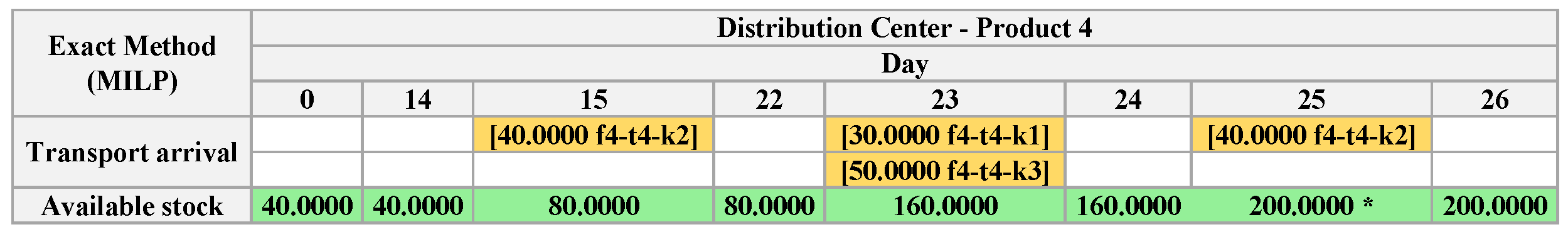
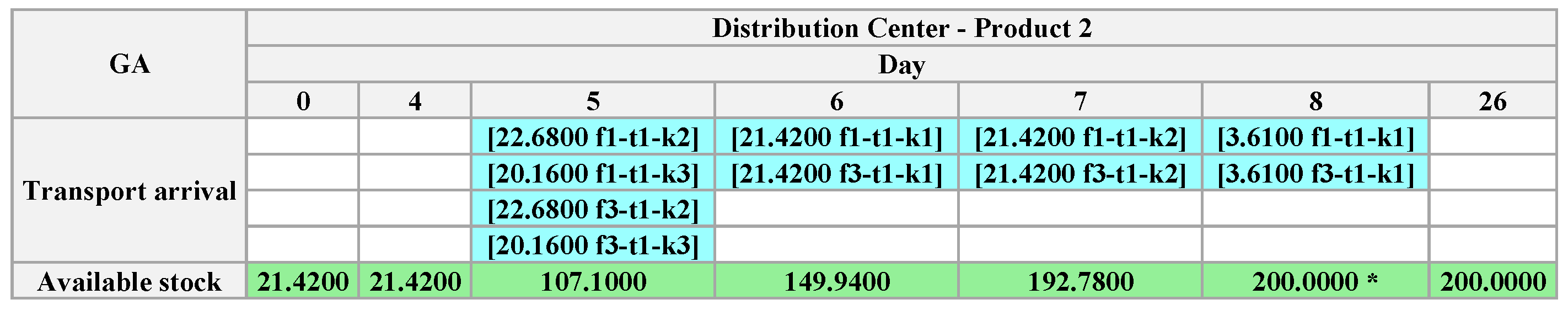
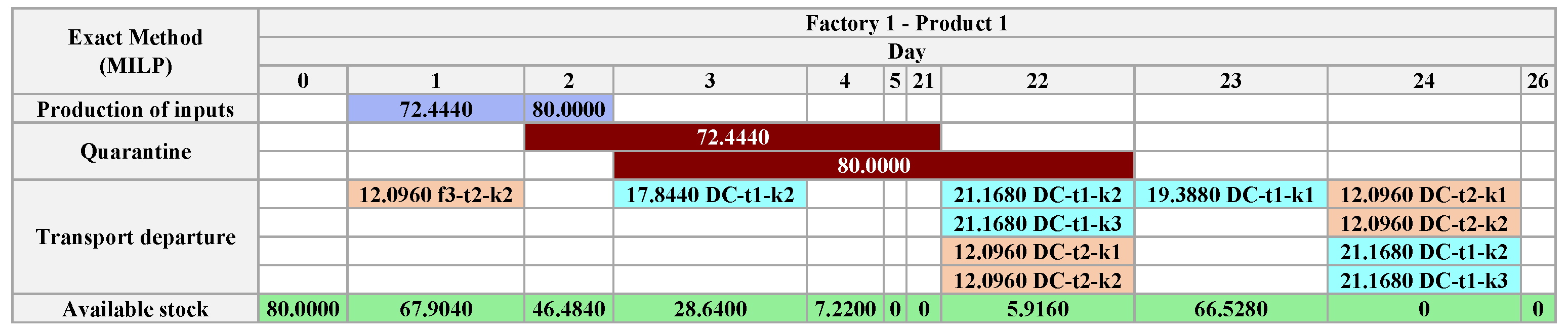
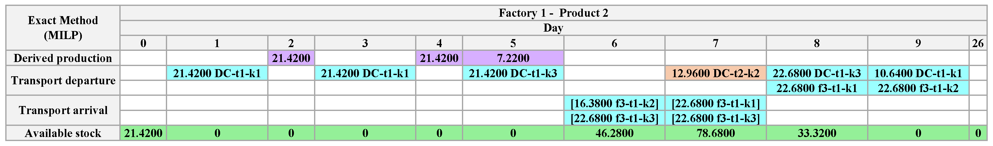
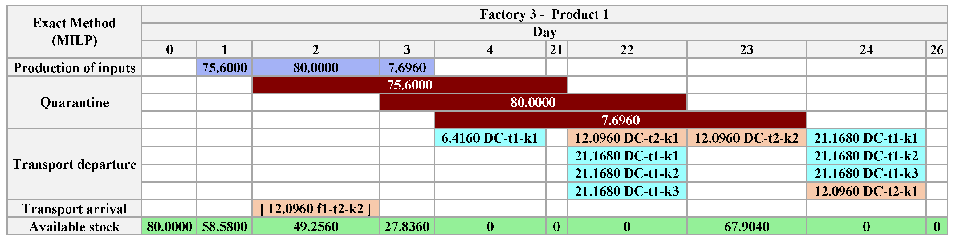
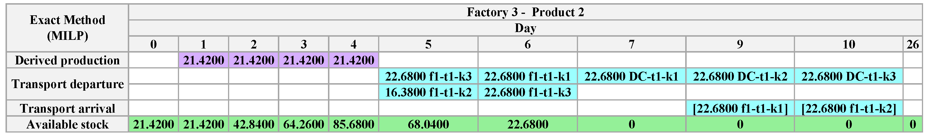
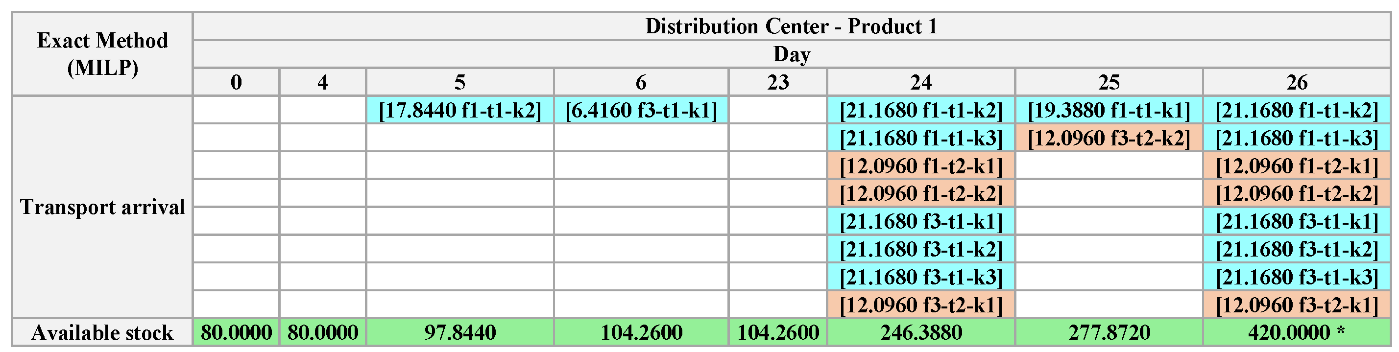
Plan Found by the Exact Method

The solution shows production planning using the Exact Method that seeks to avoid redundant factory stocks by producing and transporting the exact quantities needed to meet demand in the DC (see Figure 26, Figure 27, Figure 28, Figure 29, Figure 30 and Figure 31 and Appendix A.2).

Note that in some situations, for dependent products, the Exact Method keeps the input products in stock instead of transporting them. This decision guarantees the production of dependent products, improving the production plan.

Through Figure 26 and Figure 28, it is observed that there is transportation of products between $f_1$ and $f_3$, complementing the stock of input products in $f_3$, for the production of $p_2$. In addition, we note the transport decisions involving the transshipment of $p_2$ between factories; according to Figure 27 and Figure 29, and this situation would not occur if there were other objectives, such as minimizing CO₂.

As in the GA, the product with the longest quarantine time, $p_1$, establishes the value of $Tmax$ also on $d_{26}$. However, unlike the solution obtained by APS, the demand for $p_2$ in the DC is satisfied before $p_1$. Another consequence of the long quarantine period of $p_1$ is that the logistic operations of this product are concentrated in the final periods.

In the first 5 days, the initial stock of $p_1$, both in $f_1$ and $f_3$, is fully used as input for $p_2$ production or transported to the $DC$ (see Figure 26, Figure 27, Figure 28 and Figure 29). As $p_1$ requires 20 days of quarantine, excluding initial stocks, there are no finished inputs for the production of $p_2$ until $d_{21}$.

The following comments are anchored in the figures of Appendix A.2. At $f_1$, the stock of $p_3$ shows a sharp reduction in the first 3 days, with dedicated shipments for $DC$, resuming production again at the end of the time horizon.

It is observed that all $p_3$ originated from $f_1$ is transported directly to the $DC$. Therefore, the production of $p_4$, which depends on $p_3$, is all carried out in $f_4$.

The initial stocks of $p_3$ and $p_4$ remain at $f_4$ until $d_5$ and $d_{14}$, respectively. The $p_3$ in $f_4$ productions are available from $d_{12}$ and are used for the production of $p_4$ or transported to the $DC$. The demand for $p_3$ and $p_4$ is met in $d_{25}$.

Products $p_5$ and $p_6$ are produced and transported according to demand as quickly as possible, which happens on $d_{20}$ and $d_{22}$, respectively.

All initial stock of $p_5$ in $f_2$ goes to the $DC$ on the first day. From this, $p5$ is being released, and its transport $DC$ seeks to optimize the capacity of the vehicles (which are type 1 or 2, used simultaneously).

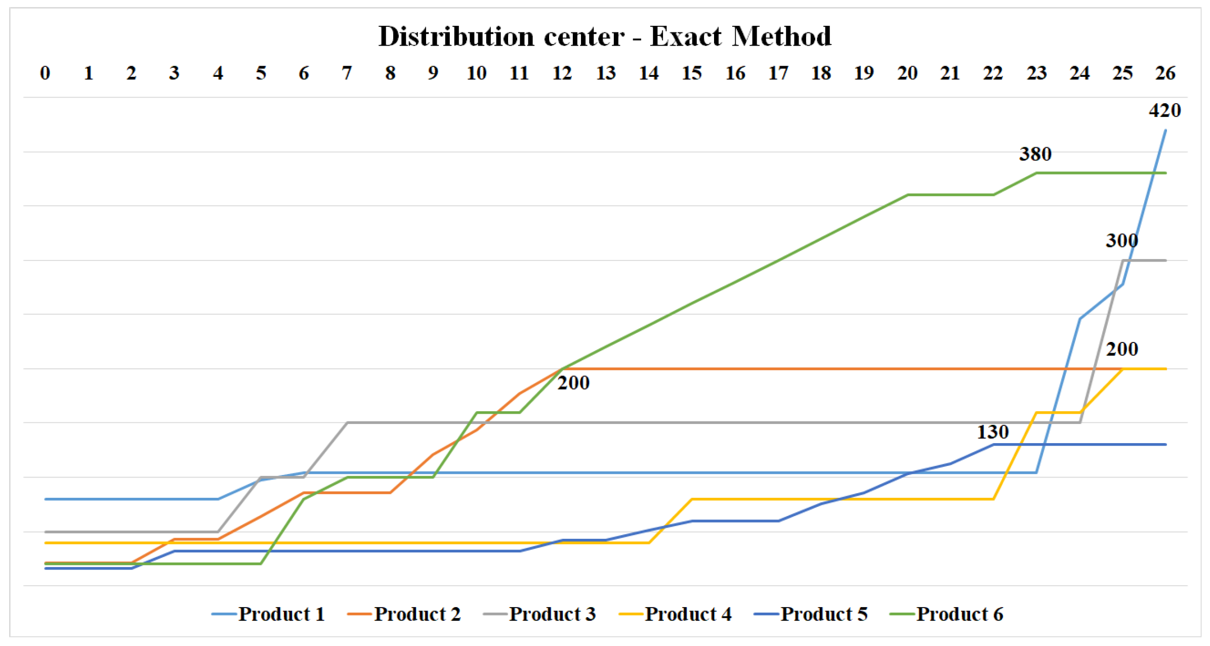
The Exact Method achieved the same result of the GA reaching a maximum completion time of 26 days. Thus, the total horizon of production and distribution of products, including all processes of production, transport, storage, and restrictions was completed in this period and demand was met accurately, with no remaining production.

The significant difference between the Exact Method and the solutions obtained by APS and the GA is that their submitted production plan ensures that finished products are made available in the distribution center with sufficient time for marketing within the shelf life.

6. Discussion of Results

Table 7. Meeting the demand for each product in days and computational effort in seconds.

P	APS	GA	Exact Method
$p_1$	44	26	26
$p_2$	65	8	12
$p_3$	10	26	25
$p_4$	16	22	25
$p_5$	39	26	22
$p_6$	41	24	22
$Tmax$	65	26	26
Time (s)	444.64 s	24.92 s	4.42 s

Bold highlights the best performance.

shows the dates when each product reaches its demand in the DC and $Tmax$ and the computational effort spent by each method.

When analyzing Table 7, it is observed that the Exact Method met the demand of most products before the other approaches in the shortest computational time. This demonstrates that for a MILP, good mathematical modeling, together with a good solver may have superior performance to other methods, especially in smaller dimensions, such as this case study.

APS required more time to meet the products’ demand requirements. New production cycles for a given product start only after the quarantine period has expired. This behavior resulted in a production plan that extrapolated the predicted time horizon.

The product $p_1$, which has the longest quarantine time and is also used as input for the production of $p_2$, determines the $Tmax$. In the Exact Method and in the GA, it was sought to meet the demand of $p_2$ while the production of $p_1$ remains in quarantine. However, in the APS, the decision was to prioritize meeting the demand of $p_1$ before supplying the demand of $p_2$, leaving its solution unfavorable.

Among the APS limitations, the computational cost due to solving complex temporal constraints and sequential decisions is worth mentioning, which significantly increases the time required to find a solution compared to the Exact Method and the GA. Since APS models problems using constraint programming, its multiple temporal and conditional dependencies contribute to expanding the search space. These factors impact both the solution time and the quality of the results, making classical approaches more competitive for this type of problem (see Table 7).

In addition, APS has accumulated a large stock of products in the factories. The GA algorithm and the Exact Method do not present residual stocks.

Figure 32, Figure 33 and Figure 34 graphically illustrate the arrival of products in the DC to meet demand.

Figure 32 shows that the decision of the APS to supply the demand of $p_1$ before $p_2$ results in a gap of 21 days where no arrival of products occurs in the DC.

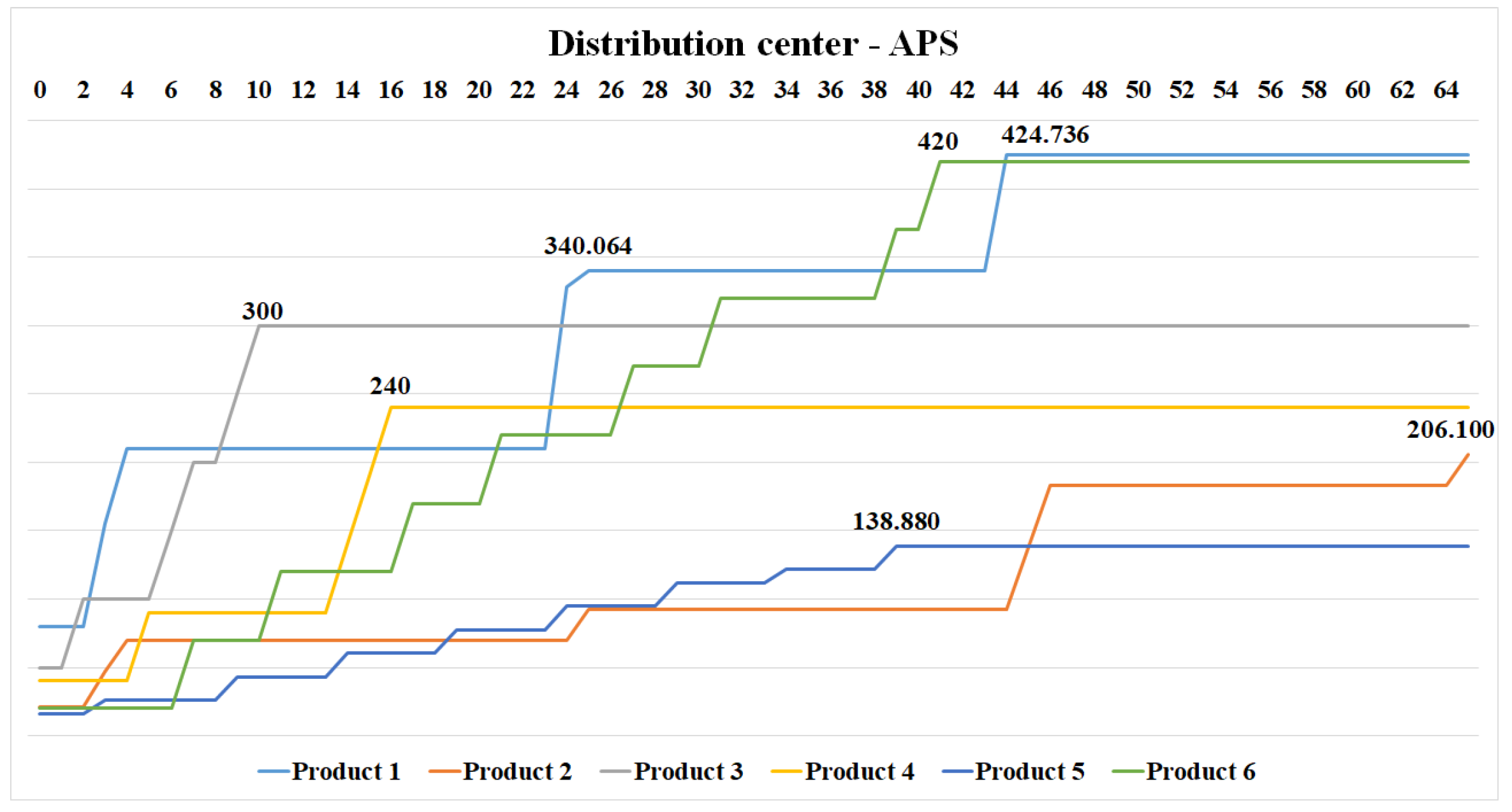
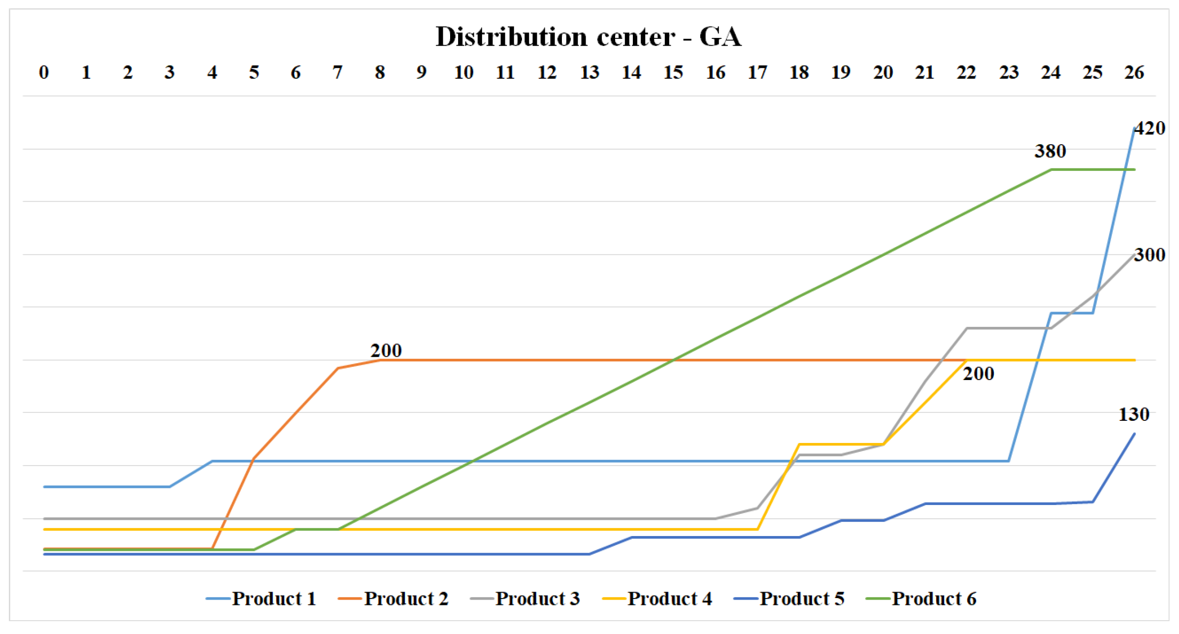
Figure 33 and Figure 34 show the increase of products in the $DC$ stock for both the GA and the Exact Method, so one can see that the demands are met within the time horizon at $d_{26}$.

The GA is more flexible in terms of modeling than the APS, although it still depends on adjustments to fit changes. The Exact Method stands out for its flexibility when adaptations are necessary. It demonstrates a more direct and efficient modeling process independent of the size of the problem. We can easily add new products and factories.

APS showed the worst performance among the three methods and did not obtain a solution nor come close to the optimal, evidencing limitations in computational efficiency and the quality of solutions found. These difficulties in obtaining the solution by APS demonstrate its ineffectiveness in treating this combinatorial optimization problem.

Although the GA is an evolutionary algorithm, it achieved the optimal result, demonstrating its capacity to explore the solutions space. The Exact Method performs best, achieving the optimal result in the shortest execution time of the compared approaches. Of course, when the problem dimension grows, achieving the optimal solution in a reasonable time will become more difficult.

It is noteworthy that APS presents a detailed report of the production plan, in addition to being open source, which facilitates its use and adaptation in different contexts. GA stands out for the availability of frameworks that facilitate and streamline the process of modeling the problem-solving algorithm. In the Exact Method, the advantage highlighted is the possibility of finding the optimal solution to the problem, ensuring a more efficient level of decision.

APS, a rigid modeling allied to the selected planner, presents severe limitations that hinder its performance and applicability in complex combinatorial problems like this MILP. The GA requires the precise coding and decoding of individuals, which are challenging and demand extensive experimentation to ensure good results. The presentation of the results obtained by the GA and the Exact Method required additional steps to decode the solutions and make them more understandable.

Finally, the importance of building a mathematical model for the problem studied is highlighted since this allows the situations and needs of the present case study to be better discussed and adequately formalized.

6.1. Computing Resources

The computational experiments were performed on a computer equipped with an Intel(R) Core(TM) i5-7200U processor, which can operate at up to 2.71 GHz, and 8 GB of RAM memory.

6.2. Data Repository

The data repository is available on GitHub and can be accessed through the link: https://github.com/docvanessaschneider/Optimization-Methods-a-Case-Study-in-a-Dairy-Industry.

7. Conclusions

The present research made relevant contributions by comparing different methodologies and tools for the dairy production chain and analyzing the advantages and limitations of each proposed approach. The scope of the optimization problem studied is limited to a case study of the dairy industry composed of four factories, six products, and one DC. The goal is to build a production and transportation plan so that the demand for each product is satisfied in the DC in the shortest possible time ($Tmax$). The following methods were compared: Automated Planning and Scheduling, a Genetic Algorithm, and an Exact Method.

We present a detailed mathematical model of the problem in question and a formulation in PDDL for the application of APS and planner OPTIC.

The high perishability of the products was treated as a central aspect in the modeling and evaluation of the solutions obtained. All products were delivered within their expiration dates. However, the solution generated by APS did not meet the demand for all products within the established planning horizon, causing problems in the retail stages. These facts demonstrate the inadequacy of APS in solving complex combinatorial problems modeled as MILP.

Considering this case study, the Exact Method presented the optimal solution with less computational effort. However, there is no guarantee that this will continue if the scale of the problem increases. The Genetic Algorithm also found the solution, standing out for its flexibility and efficiency in exploring the space of solutions. Thus, we can apply the Exact Method until the size of the problem allows, and then, a metaheuristic can be used to maintain the quality of the solution.

Future Research

For future research in the dairy production chain using Automated Planning and Scheduling, we recommend the development of a dedicated algorithm that uses all the knowledge acquired so far and can work in a hybrid way with exact solvers and metaheuristics.

In addition, the objective of maximizing production capacity in the search for the full use of factories and vehicles and minimizing idleness should be considered. Another issue is to solve the problem as multi-objective, incorporating environmental issues and emissions of $C{O}_2$, as well as avoiding the loss of products that exceed their useful life.