Article

Enhanced Wind Energy Forecasting Using an Extended Long Short-Term Memory Model

by
Zachary Barbre
and
Gang Li
*
Michael W. Hall School of Mechanical Engineering, Mississippi State University, Starkville, MS 39762, USA
*
Author to whom correspondence should be addressed.
Algorithms 2025, 18(4), 206; https://doi.org/10.3390/a18040206
Submission received: 2 March 2025 / Revised: 27 March 2025 / Accepted: 3 April 2025 / Published: 7 April 2025
(This article belongs to the Section Algorithms for Multidisciplinary Applications)

Abstract

:
This paper presents an innovative approach to wind energy forecasting through the implementation of an extended long short-term memory (xLSTM) model. This research addresses fundamental limitations in time-sequence forecasting for wind energy by introducing architectural enhancements to traditional LSTM networks. The xLSTM model incorporates two key innovations: exponential gating with memory mixing and a novel matrix memory structure. These improvements are realized through two variants, i.e., scalar LSTM and matrix LSTM, which are integrated into residual blocks to form comprehensive architectures. The xLSTM model was validated using SCADA data from wind turbines, with rigorous preprocessing to remove anomalous measurements. Performance evaluation across different wind speed regimes demonstrated robust predictive capabilities, with the xLSTM model achieving an overall coefficient of determination value of 0.923 and a mean absolute percentage error of 8.47%. Seasonal analysis revealed consistent prediction accuracy across varied meteorological patterns. The xLSTM model maintains linear computational complexity with respect to sequence length while offering enhanced capabilities in memory retention, state tracking, and long-range dependency modeling. These results demonstrate the potential of xLSTM for improving wind power forecasting accuracy, which is crucial for optimizing turbine operations and grid integration of renewable energy resources.

1. Introduction

Wind energy is essential in the global transition to sustainable energy, as it harnesses the power of wind, a renewable and abundant resource, to produce clean electricity without harmful emissions. Wind is a global phenomenon that countries around the world can tap into, and the versatility of wind production permits wind turbines to be deployed offshore as well as on land [1]. Wind energy is produced by wind turbines, which convert kinetic energy from wind into electrical power by using large blades that rotate a generator [2,3]. As one of the fastest-growing sources of renewable energy, wind turbines play a significant role in reducing reliance on fossil fuels, lowering greenhouse gas emissions, and mitigating climate change [4,5]. In the world energy arena, wind energy is the predominant renewable energy source, and wind power production more than tripled between 2010 and 2020, increasing from 198 gigawatts (GW) to 743 GW in that span [6]. Wind energy is sourced from wind farms, which feature scores of wind turbines spread out across a large area. Any effort to predict wind power production must consider the dynamics of every single wind turbine in a wind farm, which involves an immense amount of data [7]. However, several challenges must be overcome to successfully predict wind power production. Among the most significant obstacles to wind power forecasting is the variability of wind [8]. Wind power is inconsistent regardless of the characteristics of the wind farm. Even if a location with a high average wind volume is selected, power output remains susceptible to factors such as the weather and the season, which can prove disruptive to the power grid supplied by the wind farm [9]. This is a significant drawback of wind energy, as the power grid relies on a consistent power input to meet the regular power needs of the customers. Furthermore, fluctuations in wind volume decrease the efficiency of the integration of wind energy into the power grid, increasing operating costs compared with those of fossil fuels [10]. However, adjustments can be made to manage changes in operating conditions if the wind power can be predicted in advance [11]. Accordingly, the ability to accurately forecast wind power production is of immense value to the wind energy sector.
Accurate wind power prediction is challenging because the conditions of each wind farm are different. Wind power parameters, such as geography, wind turbine type, number of wind turbines, and weather patterns, differ between wind farms, which makes creating a single rigid prediction model impractical [10]. Prediction methods can be physical or statistical in nature. Physical models are supplied with weather data, including air pressure, humidity, water vapor concentrations, and air speed. These inputs are used to generate wind power output using thermodynamics, but the utility of these models is limited due to the need for up-to-date conditions and a high cost of local and imprecise data [12,13]. Statistical methods involve supplying the model with historical wind conditions and power data. These data are used to train the model to forecast site-specific wind power production based on trends and patterns identified over time [13,14]. Statistical wind power prediction methods are most effective when employing intelligent artificial intelligence (AI) algorithms featuring deep learning [15]. Those deep learning models are artificial neural networks (ANN), which include multiple hidden layers that allow the model to process inputs and determine outputs of interest, such as future wind power outputs [16]. Those deep learning models can analyze large datasets of historical weather patterns, real-time meteorological data, and turbine performance to forecast wind conditions more accurately, allowing wind farms to dynamically adjust turbine settings [17]. This approach to wind power prediction is not new, as statistical time series models, such as autoregressive integrated moving average (ARIMA) and kernel extreme learning machine (KELM), are frequently used for process prediction. More recently, deep learning models, e.g., long short-term memory (LSTM), with elements, e.g., gated recurrent units (GRU), have become more prevalent in the prediction of wind power [9]. As a special case of recurrent neural networks (RNN), LSTM has greater accuracy and fewer errors in wind power prediction relative to other methods. Convolutional neural networks (CNNs) are also used in time series prediction, although limitations include CNNs’ tendency to consider only ordinary feature extraction, while neglecting to capture time series modeling characteristics [18]. This results in maximum efficiency, improved grid integration, and reduced downtime of each turbine, which stabilizes energy production, enhances reliability of the grid, and reduces operational costs, which would help to fully unlock the potential of wind energy [19]. These AI models offer the potential for long-term wind power prediction, but limitations of existing models limit their utility.
Numerous wind power prediction methodologies using the models introduced previously have been published, each of which has made valuable contributions to advance the field. One study exploring this area is the development of a CNN-LSTM deep learning model to perform 2-D regional short-term wind speed forecasting. This study combined a CNN and LSTM to develop a model capable of forecasting wind speed more accurately than other similar models. The geographic data from the wind farm was used to train the CNN component, while the chronological data were used to train the LSTM module. The feature extraction of the CNN and historical prediction of the LSTM were input back into the CNN to predict wind speed components, with very accurate results [20]. Another study involved developing a novel genetic LSTM (GLSTM) model for wind power forecasting. This study created a GLSTM framework that combined LSTM with a genetic algorithm (GA) for short-term wind power prediction. GA is an optimization algorithm that helps address the limitations of computing power and time that wind energy prediction models require to obtain accurate results. This added optimization increases the capability of LSTM layers, which bolsters the sequential data learning capability of the existing LSTM model. Results from this study indicated average improvements between 6% and 30% compared with existing wind power prediction models, including standard LSTM [14]. Both of these models, as well as countless others, considerably bolstered the quality of wind power forecasting in the short term. However, short-term predictions only provide a wind power output outlook of days at best, whereas accurate long-range prediction of wind power would allow turbine operators to better optimize the production of power. While traditional models, such as LSTM, GRU, RNN, and ARIMA, are effective for time series prediction, they have limitations in handling highly complex, multistep forecasting tasks of the nature needed for wind power prediction [21,22]. Classic RNNs suffer from the vanishing gradient problem, hindering their ability to learn long-term dependencies in sequential data [23,24].
Beyond the above studies, some Transformer-based architectures have been used for wind power forecasting as well. A Transformer-based deep neural network incorporating wavelet transform showed promising results in 6 h ahead wind power prediction [25]. Another Transformer-based model was developed to capture long-term dependencies and key information within wind data, enabling the extraction of correlations between wind farms and wind power forecasting [26]. Wu et al. [27] used ensemble empirical mode decomposition to convert the original wind speed sequence from one to sixteen dimensions and a Transformer model to directly model the multidimensional wind speed data. A multihead attention mechanism within Transformer neural networks was developed in [28] to learn sequential dependencies between wind turbines to qualify spatial information. Xiang et al. [29] combined LSTM with a vision Transformer model to better utilize the relationship between extracted characteristics and the desired output for accurate prediction. While the above Transformer-based models represent improvements from traditional LSTM and GRU architectures, their high computational cost for large quantities of wind power data is a concern. The input to the prediction model is enormous, and while performing a time series analysis, further data are produced that must also be stored and remembered. Mechanisms, e.g., GRUs [30] and empirical mode decomposition [16], permit previous information to be discarded and decomposited, and while the LSTM architecture does not permit the complete discarding of past information, losses do occur, which affects the quality of the prediction. To improve the performance of LSTM, particularly for memory and data storage concerns, further modification of the LSTM model is required, which introduces the need for extended LSTM (xLSTM).
xLSTM improves upon these models by incorporating additional layers and mechanisms, such as attention mechanisms, to capture more intricate temporal dependencies and better handle non-linear relationships in the data. This results in improved accuracy, particularly for long-range predictions in energy systems. The proposed xLSTM architecture further extends this paradigm by implementing a dual-pathway approach that combines scalar and matrix memory structures, thereby addressing the inherent limitations of conventional recurrent models in capturing multiscale temporal patterns in wind energy data. Moreover, the empirical validation conducted across diverse seasonal conditions demonstrates the xLSTM model’s robustness and adaptability to varying meteorological phenomena, establishing a foundation for more reliable integration of intermittent renewable energy sources into existing power grid infrastructures.
The remainder of this paper is organized as follows: Section 2 presents the xLSTM architecture, including detailed formulations of both sLSTM and mLSTM components. Section 3 outlines the SCADA data processing methodology for wind power forecasting, encompassing data preprocessing, quality control procedures, and hyperparameter optimization strategies. Section 4 presents the empirical results of the xLSTM model implementation, with detailed analyses of prediction accuracy across various wind speed regimes and seasonal patterns. Finally, Section 5 summarizes the major findings, discusses the implications for wind energy forecasting applications, and proposes directions for future research development.

2. Extended Long Short-Term Memory Networks

The architectural enhancement of xLSTM to traditional LSTM networks introduces two key improvements, i.e., exponential gating with memory mixing and a novel matrix memory structure. The architecture of the xLSTM model achieves these improvements through two variants, i.e., a scalar LSTM (sLSTM) model and a matrix LSTM (mLSTM) model. The sLSTM model enhances the traditional architecture of LSTM networks by implementing exponential gating mechanisms alongside a new memory mixing technique, enabling more effective revision of stored information through scalar cell states while maintaining the xLSTM model’s tracking capability for complex time-sequence dependencies. The mLSTM model replaces scalar memory cells with matrix-valued states, incorporating a covariance update rule for key-value associations, which expands the xLSTM model’s storage capacity while enabling parallel computation through matrix operations. These sLSTM and mLSTM models are integrated into residual blocks and stacked to form comprehensive architectures. The xLSTM model maintains linear computational complexity with respect to sequence length while offering enhanced capabilities in memory retention, state tracking, and long-range dependency modeling.

2.1. sLSTM Model

The sLSTM model is developed with exponential gating and normalized memory updates to enhance conventional LSTM networks. The memory cell update in sLSTM at time t can be obtained by the cell state equation, which can be represented as
c t = f t c t 1 + i t z t ,
where c t R d represents the cell state at time t, f t denotes the forget gate output, i t is the input gate output, and  z t represents the cell input. To maintain proper scaling of cell states, sLSTM implements a normalizer state:
n t = f t n t 1 + i t ,
where n t R d represents the normalizer state that accumulates gating operation effects over time. The sLSTM model processes input information through a cell input, which is
z t = ϕ ( ω z x t + r z h t 1 + b z ) ,
where x t R m is the input vector, ω z represents the input weight matrix between inputs x t and the cell input, r z is the recurrent weight between the hidden state value h t 1 and the cell input, b z is the bias term, and  ϕ ( · ) is the cell input state activation function.
The normalized hidden state value in sLSTM can be represented as
h t = o t c t n t ,
where h t is the hidden state value and o t represents the output gate value in sLSTM. The gating mechanism of the sLSTM model comprises three components, i.e., input, output, and forget gates. The input gate in sLSTM employs exponential activation, which can be represented as
i t = exp ω i x t + r i h t 1 + b i ,
where ω i represents the input weight matrix between inputs x t and the input gate, r i is the recurrent weight between the hidden state value h t 1 and the input gate, and  b i is the scalar bias of the input gate. The forget gate in sLSTM allows flexibility in activation choice, which can be represented as
f t = γ ω f x t + r f h t 1 + b f ,
where ω f represents the forget weight matrix between inputs x t and the forget gate, r f is the recurrent weight between the hidden state value h t 1 and the forget gate, b f is the scalar bias of the forget gate, and γ ( · ) represents either sigmoid σ or exponential activation. The output gate in sLSTM uses sigmoid activation, which is
o t = σ ω o x t + r o h t 1 + b o ,
where ω o represents the output weight matrix between inputs x t and the output gate, r o is the recurrent weight between the hidden state value h t 1 and the output gate, and  b o is the scalar bias of the output gate.
To ensure numerical stability with exponential activations, sLSTM incorporates a stabilization mechanism, which is
m t = max ( log ( f t ) + m t 1 , log ( i t ) ) ,
where m t R is the scalar stabilizer state in sLSTM. Equation (8) enables the computation of stabilized input and forget gate values, which are
i t = exp log ( i t ) m t
f t = exp log ( f t ) + m t 1 m t ,
where i t and f t represent stabilized input and forget gates in sLSTM, respectively.

2.2. mLSTM Model

The mLSTM model extends xLSTM by upgrading scalar cell states c t in Equation (1) to matrix memory cell states C t R d × d , which enables enhanced storage capacity and parallel computation. The core innovation of mLSTM lies in its matrix memory cell state update using a covariance-based update rule, which can be represented as
C t = f t C t 1 + i t v t k t ,
where C t represents the matrix memory cell state at time t, f t is the forget gate vector in mLSTM, and v t and k t represent value and key vectors, which are
v t = W v x t + b v
k t = 1 d ( W k x t + b k )
respectively, in which W v is the weight matrix between the value vector and the input vector, W k are the weight matrix between the key vector and the input vector, b v and b k represent bias vectors for the value and key vectors, respectively, and d is the dimension of the key/value space in the matrix memory.
The normalizer state tracks the cumulative effect of key vectors k t weighted by gates. The normalizer state vector in the mLSTM model can be represented as
n t = f t n t 1 + i t k t ,
where n t 1 represents the normalizer state vector at time t 1 . The matrix hidden state computation in mLSTM involves query-based memory retrieval, which is
h t = o t h ˜ t ,
where o t is the output gate vector in mLSTM, ⊙ denotes element-wise multiplication, and  h ˜ t can be represented as
h ˜ t = C t q t max n t q t , 1 ,
in which q t is the query vector. The query vector is computed from the input:
q t = W q x t + b q ,
where W q is the weight matrix between the input vector and the query vector and b q is the bias vector.
The gating mechanism employs exponential activation for the input gate:
i t = exp W i x t + b i .
The forget gate allows for either sigmoid or exponential activation:
f t = γ W f x t + b f ,
where ω f R m represents the forget gate weight matrix, b f is the bias vector for the forget gate, and γ denotes either sigmoid σ or exponential activation. The output gate vector of mLSTM can be represented as
o t = σ W o x t + b o ,
where W o R d × m represents the output gate weight matrix and b o R d is the bias vector for the output gate vector. Algorithm 1 captures the essential computational flow of the xLSTM model, incorporating both the sLSTM and mLSTM variants.
Algorithm 1 xLSTM forward pass with sLSTM and mLSTM components
1:
Initialize: Cell state C 0 = 0 , hidden state h 0 = 0 , normalizer state n 0 = 0 , stabilizer state m 0 = 0
2:
for  t = 1 to T do
3:
    SCADA data preprocessing
4:
    Compute cell input: z t = ϕ ( ω z x t + r z h t 1 + b z )
5:
    if using sLSTM variant then
6:
        Cell input computation
7:
         z t = ϕ ( z ˜ t )
8:
         z ˜ t = ω z x t + r z h t 1 + b z
9:
        Input gate computation
10:
         i t = exp ( i ˜ t )
11:
         i ˜ t = ω i x t + r i h t 1 + b i
12:
        Forget gate computation
13:
         f t = γ ( f ˜ t )
14:
         f ˜ t = ω f x t + r f h t 1 + b f
15:
        Output gate computation
16:
         o t = σ ( o ˜ t )
17:
         o ˜ t = ω o x t + r o h t 1 + b o
18:
        Cell state update
19:
         c t = f t c t 1 + i t z t
20:
        Normalizer state update
21:
         n t = f t n t 1 + i t
22:
        Hidden state computation
23:
         h t = o t c t n t
24:
        Gate stabilization mechanism
25:
         m t = max ( log ( f t ) + m t 1 , log ( i t ) )
26:
         i t = exp ( log ( i t ) m t )
27:
         f t = exp ( log ( f t ) + m t 1 m t )
28:
    end if
29:
    if using mLSTM variant then
30:
        Compute query, key, and value vectors:
31:
         q t = W q x t + b q
32:
         k t = 1 d ( W k x t + b k )
33:
         v t = W v x t + b v
34:
        Compute gates:
35:
         i t = exp ( W i x t + b i )
36:
         f t = γ ( W f x t + b f )
37:
         o t = σ ( W o x t + b o )
38:
        Matrix memory update:
39:
         C t = f t C t 1 + i t ( v t k t )
40:
         n t = f t n t 1 + i t k t
41:
         h t = o t C t q t max ( | n t q t | , 1 )
42:
    end if
43:
end for

3. SCADA Data Processing for for xLSTM

3.1. SCADA Data Processing for Wind Power Forecasting

Supervisory control and data acquisition (SCADA) technology enables comprehensive monitoring of operational parameters in wind power systems. For wind turbine performance analysis, SCADA systems collect two distinct categories of information: sensor measurements and operational status codes [31]. The sensor-based data encompasses critical performance metrics, including power generation levels, rotational velocities, pitch angle positions, mechanical vibrations, thermal conditions, and lubricant properties. Meanwhile, status code information provides detailed event logging and state notifications regarding various turbine subsystems and components. These diagnostic codes vary across different original equipment manufacturers (OEMs) but serve to document the operational conditions and health status of the turbine. The systematic collection and analysis of both sensor measurements and status notifications through SCADA infrastructure facilitates real-time performance assessment and operational diagnostics of wind power assets. This integrated monitoring approach supports data-driven decision-making for optimizing turbine operation and maintenance strategies.
To prepare SCADA data for wind power forecasting, a systematic preprocessing approach is implemented. Raw SCADA data in Table 1 are initially collected at 10 min sampling intervals, including key wind feature parameters, such as turbine rotational speeds, power outputs, and yaw angles. For a single wind turbine, its SCADA data yield approximately 50,530 data arrays over a one-year operational period. Quality control procedures identify and remove anomalous measurements, including missing values and statistical outliers, resulting in a refined dataset of 47,316 valid data arrays. This processed dataset undergoes temporal partitioning, with 80% of the seasonal data designated for model training and the remaining 20% allocated for testing purposes. To enhance model performance, the SCADA data undergo normalization to standardize the scale of different operational parameters. Additionally, the SCADA data processing incorporates validation checks to ensure temporal consistency and proper handling of sensor measurement boundaries. This rigorous data preparation framework ensures the reliability and representativeness of SCADA measurements for predictive models.
Figure 1 uses a polar coordinate system where each point’s radial distance from the center represents wind speed magnitude, while its angular position corresponds to wind direction. The statistical analysis reveals that the wind regime at the monitoring location is characterized by a mean wind speed of 7.56 m/s, with values ranging from complete calm (0.00 m/s) to substantial gusts (25.21 m/s). The median wind speed of 7.10 m/s indicates a slightly right-skewed distribution. The point distribution demonstrates distinct directional preferences, with the highest frequency of occurrence (7995 observations) concentrated in the east-northeast sector (67.5°). This predominant wind direction constitutes approximately 15.8% of all recorded measurements.
This directional and magnitude characterization provides essential contextual information for interpreting SCADA measurements and enhancing the precision of xLSTM-based power output predictions. The significant proportion of measurements exceeding 6 m/s (60.6% cumulatively) suggests favorable conditions for energy generation, while the well-defined directional prevalence enables more precise modeling of the relationship between meteorological variables and power output.
Table 2 presents a categorization of SCADA data distributed across eight directional sectors, each spanning 45° of wind directions. This SCADA data organization facilitates analysis of data quality and distribution patterns across different wind directions, which is crucial for accurate wind power forecasting models. Identifying and removing outliers in SCADA data serves to eliminate atypical measurements that could otherwise distort the underlying statistical distributions and compromise the validity of predictive models. These anomalous data points, which may result from sensor malfunctions, communication errors, or extreme environmental conditions, must be systematically detected and excluded to establish a more representative dataset that accurately reflects normal operational patterns of wind turbines.
The raw SCADA dataset comprises 50,530 data points collected over a one-year monitoring period, as shown in Table 2. In the data preprocessing pipeline, outlier identification was implemented through statistical thresholds and domain-specific constraints that flag measurements deviating significantly from established operational patterns. A combination of univariate and multivariate methods was used for outlier identification of the SCADA data, including interquartile range analysis, modified z-score calculations with thresholds of ± 3.5 , and physics-based validation rules that identify physically impossible or improbable parameter combinations, e.g., power generation during zero wind speed conditions, or power outputs exceeding theoretical maximums defined by the Betz limit. Through rigorous quality control procedures, 3214 data points (approximately 6.36% of the total) were identified as outliers and subsequently removed from the following xLSTM training for wind power forecasting. The resulting refined dataset consists of 47,316 valid SCADA measurements.
Analysis of the wind directional distribution in the dataset reveals significant spatial heterogeneity in measurement frequency. The quadrants of 180°–270° and 270°–315° collectively exhibit the highest sampling density, comprising 16,674 measurements or 33.0% of the total dataset. This non-uniform distribution corresponds to the prevailing wind patterns at the wind turbine location, which predominantly originate from these directions. In contrast, the quadrant of 90°–135° demonstrates minimal representation in the dataset with only 4795 measurements, which constitutes 9.5% of the total SCADA dataset.
Statistical examination of outlier distribution in the SCADA dataset reveals a remarkably consistent proportion across all directional sectors, with outlier prevalence ranging between 6.34% and 6.36% of sector-specific measurements. This uniformity in outlier distribution suggests that data anomalies manifest independently of wind directions, pointing toward systematic instrumentation issues or processing errors rather than direction-dependent measurement inaccuracies. The categorization of data according to directional sectors facilitates the implementation of sectorally differentiated modeling approaches, enabling directionally sensitive parameter optimization and enhanced predictive accuracy for wind power forecasting applications.

3.2. Hyperparameter Tuning for xLSTM

Hyperparameter optimization for the xLSTM architecture constitutes a critical determinant of model performance when applied to SCADA data analytics for wind power forecasting. The multifaceted architectural components of xLSTM, including sLSTM and mLSTM with their respective exponential gating mechanisms and matrix memory structures, necessitate systematic calibration of numerous interdependent parameters to achieve optimal predictive accuracy. This calibration process extends beyond conventional neural network parameterization to encompass specific considerations for xLSTM, e.g., head dimensionality, the number of heads per layer, block-specific projection factors, forget gate initialization strategies, and the optimal ratio of mLSTM to sLSTM blocks within the composite architecture. Given the temporal complexity and non-stationary characteristics inherent in wind turbine SCADA data, including diurnal variations, seasonal patterns, and stochastic atmospheric phenomena, a methodical hyperparameter optimization framework was implemented to maximize the xLSTM model’s capacity to capture both short-term fluctuations and longer-term dependencies in the multidimensional parameter space of wind power generation.

3.2.1. Hyperparameter Optimization for sLSTM Configuration

For sLSTM, hyperparameter optimization focuses on maximizing the efficiency of the scalar memory mechanism and exponential gating structure. The tuning process prioritizes parameters that influence the sLSTM model’s ability to revise storage decisions and facilitate effective memory mixing across multiple heads. Critical parameters include the head size, which determines the dimensionality of each attention head’s representation space, and the projection factor that controls the expansion ratio in the feed-forward network within each block. The number of heads per layer requires careful calibration to balance computational complexity against the xLSTM model’s capacity to capture diverse temporal patterns in wind power generation data. Additionally, the initialization strategy for forget gates proves particularly crucial for stabilizing the exponential gating mechanism and ensuring consistent gradient flow during training. Hyperparameter optimization for sLSTM involves a multifaceted approach that addresses the unique architectural components of scalar memory and exponential gating mechanisms.
A systematic grid search across parameter spaces, complemented by Bayesian optimization techniques is used for fine-tuning hyperparameters of sLSTM within promising regions, as listed in Table 3. The head size parameter demonstrated a critical inflection point at 32, with dimensions below this threshold, i.e., ( 16 , 24 ) , resulting in 7–12% higher validation errors due to insufficient representational capacity, while larger dimensions of ( 48 , 64 ) yielded diminishing returns (less than 1.2% improvement) at substantially increased computational cost (42–78% longer training times). The projection factor of 4/3 emerged as optimal through systematic ablation studies comparing values in the range of [ 1.0 , 1.33 , 1.5 , 2.0 ] , with this specific value balancing model expressivity and computational efficiency—particularly for capturing rapid meteorological fluctuations. Additionally, forget gate initialization within the range of [ 3 , 6 ] proved crucial for maintaining gradient stability during training, with values outside this range resulting in convergence difficulties, especially when processing long temporal dependencies characteristic of seasonal wind patterns.

3.2.2. Hyperparameter Optimization for mLSTM Configuration

Hyperparameter optimization of the mLSTM model, as listed in Table 4, centers on enhancing the matrix memory capabilities and covariance update mechanisms. Tuning focuses on parameters that govern the interaction between query–key–value transformations and the matrix memory structure, which directly impacts the mLSTM model’s capacity to store and retrieve temporal dependencies in wind turbine operational data. Essential parameters include the matrix memory dimension, which determines the storage capacity for temporal patterns, and the projection factor that influences the mLSTM model’s ability to capture complex relationships in high-dimensional spaces. The configuration of these parameters significantly affects the mLSTM model’s ability to process parallel sequences and maintain effective information flow through the covariance update rule.
For the mLSTM configuration detailed in Table 4, hyperparameter sensitivity was most pronounced in the matrix memory dimension and projection factor parameters. The matrix memory dimension of 128 was selected after evaluating values between 64 and 256, with performance plateauing above 128 while computational requirements increased quadratically. Unlike sLSTM, the projection factor parameter of mLSTM was optimized at 2.0 within the range of [ 1.5 , 2.0 , 2.5 , 3.0 ] . The projection factors below 2.0 limited representational capacity (decreasing R 2 by 3–5%), while higher values led to parameter redundancy without significant accuracy improvements. The selected batch size of 32 maximizes GPU memory utilization efficiency with the specified matrix memory dimensions, achieving near-optimal throughput (96% of the theoretical maximum) on the employed hardware configuration. This comprehensive parameter sweep enabled the identification of configuration values that maximize the complementary strengths of both sLSTM and mLSTM components within the unified xLSTM architecture.

4. Results and Discussion

4.1. xLSTM Results for Wind Energy Forecasting

4.1.1. Model Evaluation Criteria

The experimental validation used a substantial SCADA dataset following preprocessing and outlier removal procedures. After removing 3214 anomalous entries from the initial 50,530 data points, the analysis proceeded with 47,316 valid SCADA measurements. To ensure robust model evaluation, these measurements underwent systematic partitioning: 80% of the seasonal data were allocated for training the xLSTM model, while the remaining 20% were reserved for independent validation purposes. This deliberate segregation of training and validation sets facilitated a comprehensive assessment of the xLSTM model’s predictive capabilities across different seasonal patterns and operational conditions.
Multiple evaluation metrics were implemented to systematically assess the xLSTM model’s capability in predicting wind power output based on SCADA data. These criteria comprehensively evaluate the xLSTM model’s performance across different operational conditions and temporal scales. The mean absolute percentage error (MAPE) quantifies the average percentage deviation between predicted and actual wind power outputs:
ϵ = 1 n i = 1 n P i P ^ i P i × 100 % ,
where P i represents the actual power output recorded in SCADA data, P ^ i denotes the xLSTM-predicted power value, and n indicates the total number of SCADA measurements in the validation dataset. The root mean square error (RMSE) measures the standard deviation of power prediction residuals:
ξ = 1 n i = 1 n ( P i P ^ i ) 2 .
For real-time SCADA-based monitoring applications, the mean absolute error (MAE) calculates the average magnitude of power prediction errors:
σ = 1 n i = 1 n | P i P ^ i | .
The coefficient of determination ( R 2 ) evaluates how effectively the xLSTM model captures variations in wind power output:
R 2 = 1 i = 1 n ( P i P ^ i ) 2 i = 1 n ( P i P ¯ ) 2 ,
where P ¯ represents the mean of actual power measurements from SCADA data.

4.1.2. xLSTM Results

The xLSTM model is configured for short-term wind power forecasting with a temporal horizon of 1–6 h. In the experimental setup, the xLSTM model processes input sequences of length 8, which represent 80 min of SCADA data at 10 min sampling intervals, to generate predictions for the next time step. This study evaluates multistep forecasting capabilities at incremental steps between 1–6 h (6–36 prediction intervals), which corresponds to the critical short-term operational planning window for wind farm management and grid integration.
The power–wind speed characteristic exhibits the expected sigmoidal pattern typical of wind turbine performance.At low wind speeds (<5 m/s), minimal power generation occurs as these velocities approach the cut-in threshold of the turbine. The power generation increases rapidly in mid-range wind speeds (between 5–12 m/s), displaying a near-cubic relationship with wind velocity, which aligns with fundamental aerodynamic principles. At higher wind speeds (>12 m/s), the power output plateaus around 3500 kW, indicating the rated capacity of the turbine has been reached, after which pitch control mechanisms maintain relatively constant power output despite increasing wind speeds.
The xLSTM-predicted power values demonstrate the xLSTM model’s capability to capture underlying patterns in the actual power production data, as shown in Figure 2. xLSTM prediction results closely follow the central tendency of the actual power measurements while exhibiting less extreme deviations than the SCADA values. This suggests that the xLSTM model effectively captures the primary relationship between wind speed and power output while filtering out some of the stochastic variations present in the real-world measurements. In the mid-range wind speeds (7–12 m/s), where the power curve exhibits its steepest gradient, both the SCADA measurements and xLSTM predictions display the greatest variance. This heightened variability is attributable to the sensitivity of power production to small fluctuations in wind speed within this transitional region. The xLSTM model appears to slightly overestimate power production at the lower end of this range (7–9 m/s) and underestimate it at the higher end (10–12 m/s), indicating potential areas for model refinement. The convergence of all three data series at low (<5 m/s) and high (15–20 m/s) wind speeds demonstrates the xLSTM model’s robust performance at the extremes of the operational wind speed range. The clustering of points near the theoretical maximum capacity indicates that the xLSTM model effectively captures the power limitation mechanisms that prevent exceeding the rated capacity during high wind conditions.
The comparative analysis of wind velocity distributions across seasonal patterns reveals insights into the predictive capabilities of the xLSTM model relative to actual SCADA measurements, as shown in Figure 3. The winter distribution exhibits a predominant unimodal pattern with peak probability density occurring at approximately 7–8 m/s, as shown in Figure 3a. Both SCADA measurements and xLSTM predictions demonstrate remarkably similar distribution shapes, with the model accurately capturing the central tendency and overall distribution profile of the empirical data. The close alignment of the density curves indicates high predictive fidelity during cold-weather operational conditions, which typically feature more consistent wind patterns. The slight variations observed at wind speed ranges of 5–7 m/s and 12–14 m/s are minimal and do not represent statistically significant deviations. Spring distributions reveal a more complex bimodal pattern with a primary concentration at 3–4 m/s and a secondary peak at approximately 8–10 m/s, as shown in Figure 3b. This bimodality reflects the transitional nature of spring weather patterns. The xLSTM model demonstrates good predictive performance across most of the distribution, though minor discrepancies are evident in the relative heights of the primary peaks. The model slightly underestimates probability density in the 3–4 m/s range while marginally overestimating it in the wind speed range of 10–11 m/s. These deviations likely correspond to the challenges in modeling transitional seasonal patterns characterized by greater meteorological variability.
The summer distribution presents a broader, more diffuse pattern with maximum probability density occurring around 6–7 m/s, as shown in Figure 3c. The xLSTM predictions closely track SCADA measurements across most of the distribution range, with particularly accurate modeling of the central peak and the tail behavior beyond 12 m/s. The model captures the characteristic summer wind pattern that typically features moderate velocities with gradual distribution tails. Minor variations appear in the 2–4 m/s range, where the model slightly underestimates probability density compared with actual SCADA measurements. Autumn exhibits the most complex distribution pattern with a primary concentration in the wind speed range of 3–6 m/s and secondary modes at approximately 10–12 m/s, as shown in Figure 3d.
This multimodal structure reflects the variable wind conditions characteristic of autumn. The xLSTM model demonstrates strong predictive performance across most velocity ranges, accurately capturing both the primary concentration and the secondary modes. However, there are minor discrepancies in the exact positioning of the peaks, with the model estimating a slightly higher probability density at 5 m/s compared with the measured peak at 4 m/s. The comparative analysis of power output distributions across seasonal patterns offers critical insights into performance characteristics of the xLSTM model for predicting wind turbine power generation, as shown in Figure 4. This analysis examines the probabilistic distribution of power output data across four distinct seasonal contexts, with particular attention to the bimodal distribution patterns that characterize wind turbine power generation. The winter season power distribution exhibits a distinctive bimodal structure with significant probability density concentrations at the extremes of the power spectrum, as shown in Figure 4a. A substantial probability density concentration exists near zero output (0–200 kW), corresponding to wind speeds below the cut-in threshold or turbine curtailment during winter weather events. Simultaneously, a secondary peak appears at rated power (3.5 MW), representing periods of optimal wind conditions. Between these extremes lies an extended transitional region (500–3000 kW) with relatively uniform and low-density distribution. The xLSTM model demonstrates excellent fidelity in capturing this bimodal structure, with a notably accurate estimation of both the near-zero and rated power probability masses. The spring distribution maintains the bimodal characteristics observed in winter but exhibits several distinctive features, as shown in Figure 4b. A more pronounced concentration appears at near-zero output (0–200 kW), with a probability density of approximately 0.002, significantly higher than other seasons. A reduced but still prominent secondary peak exists at the rated power of the wind turbine, with a density of approximately 0.0009.
The summer power distribution reveals a modified bimodal pattern with unique characteristics. A reduced but still significant probability density appears at near-zero output (0–200 kW), with a density of approximately 0.00160. A less pronounced secondary peak exists at rated power, with a density of approximately 0.00060. The distribution shows a more substantial probability mass in the intermediate power ranges (500–1000 kW), indicating more frequent operation at partial load conditions. The autumn distribution exhibits distinctive features that differentiate it from other seasons. A substantial probability density at near-zero output (0–200 kW) appears similar to spring conditions but with a slightly lower magnitude (≈0.0019). A moderate secondary peak exists at rated power, with a density of approximately 0.00065. The power distribution shows an increased probability mass in the range of 2000–3000 kW relative to other seasons, which indicates more variable power generation.

4.2. Discussion of xLSTM Results

4.2.1. Time Series Prediction Performances of xLSTM for Wind Power Prediction

The performance assessment of the xLSTM model for wind power output prediction reveals promising capabilities across various wind speed regimes, as shown in Figure 2. The xLSTM model demonstrates varying prediction accuracy depending on wind speed conditions, as quantified in Table 5. At low wind speeds (0–5 m/s), the model achieves an R 2 value of 0.886, indicating substantial correlation between predicted and actual values despite the inherent variability in this operational range. The MAPE in this region stands at 9.65%, with relatively low RMSE of 32.7 kW and MAE of 29.4 kW that reflect the xLSTM model’s capacity to manage the stochastic nature of low wind conditions.
In the medium wind speed range (5–12 m/s), which encompasses the steepest portion of the power curve where minor speed fluctuations produce significant power output changes, the xLSTM model maintains robust performance with an R 2 value of 0.901. This range exhibits the highest absolute errors (RMSE of 35.5 kW and MAE of 47.8 kW) and MAPE (11.83%), attributable to the rapid rate of change in power output relative to wind speed in this transition region.
The xLSTM model achieves its strongest predictive accuracy in the high wind speed range (>12 m/s), with an R 2 value of 0.954 and a notably low MAPE of 4.21%. This enhanced performance corresponds to the plateau region of the power curve where output stabilizes, resulting in relatively modest RMSE of 34.2 kW and MAE of 42.6 kW despite the higher power magnitudes involved.
Aggregating across all wind speed ranges, the xLSTM model achieves comprehensive performance metrics of R 2 = 0.923, MAPE ϵ = 8.47%, RMSE ξ = 34.6 kW, and MAE σ = 36.2 kW. These values indicate a strong overall predictive capability with particularly robust performance at high wind speeds where power generation reaches maximum capacity. The xLSTM model’s distinct performance characteristics across different wind speed regimes highlight its adaptability to the non-linear relationship between wind speed and power output. This graduated performance profile suggests potential enhancements through regime-specific optimization strategies or ensemble approaches combining specialized models for each operational range.

4.2.2. Seasonal Wind Speed Distribution Prediction Performances

The comparative analysis of wind velocity distributions between SCADA measurements and xLSTM predictions yields significant insights across all four seasons, as shown in Table 6. The winter distribution exhibits predominantly unimodal characteristics with high prediction accuracy. The primary mode appears at 7.8 m/s in SCADA measurements versus 7.5 m/s in xLSTM predictions, demonstrating a 3.8% deviation. Central tendency measures show strong agreement, with mean wind speeds of 8.2 m/s and 8.1 m/s for SCADA and xLSTM, respectively. The distribution shape parameters indicate similar patterns between measured and predicted data, with coefficients of variation (0.58 for SCADA measurements, 0.57 for xLSTM results) and skewness values (0.67 for SCADA measurements, 0.64 for xLSTM results) showing minimal discrepancy. The exceptional model performance is further validated by an R 2 value of 0.987 and a low MAPE of 4.3% in probability density estimation.
Spring distributions present more complex bimodal patterns, reflected in their high bimodality coefficients (0.59 for SCADA measurements, 0.56 for xLSTM results). The primary mode occurs at 3.4 m/s in SCADA measurements versus 3.6 m/s in xLSTM predictions, while the secondary mode shows greater deviation (8.2 m/s for SCADA measurements, 8.8 m/s for xLSTM results). Distribution shape parameters demonstrate slightly higher divergence compared with other seasons, with standard deviations of 5.1 m/s (SCADA) versus 5.3 m/s (xLSTM). This increased complexity is reflected in the highest MAPE value (8.7%) and RMSE (0.038) among all seasons, though the R 2 value of 0.963 still indicates a strong correlation. The probability of wind speeds below 5 m/s shows a notable difference (0.42 for SCADA measurements, 0.38 for xLSTM results), suggesting a 9.5% underestimation of low-wind conditions by the xLSTM model.
Summer distributions reveal strong alignment in central tendency metrics, with mean and median wind speeds differing by only 2.7% and 1.5%, respectively. The unimodal structure (bimodality coefficient: 0.47 for SCADA, 0.45 for xLSTM) shows consistent representation between measured and predicted distributions, with primary mode probability densities closely matched (0.099 for SCADA measurements, 0.102 for xLSTM results). Distribution shape characteristics show remarkable consistency in dispersion patterns (standard deviation: 4.3 m/s for SCADA measurements, 4.2 m/s for xLSTM results) and coefficient of variation (0.59 for both). Performance metrics confirm this strong alignment with an R 2 value of 0.978 and an MAPE of 5.2%, positioning summer as the second-best predicted season after winter.
Autumn presents a moderately bimodal structure (bimodality coefficient: 0.53 for SCADA measurements, 0.51 for xLSTM results) with the most significant modal shift among all seasons (primary mode: 3.5 m/s for SCADA measurements, 4.8 m/s for xLSTM results). Despite this modal displacement, other central tendency measures show closer agreement (mean: 6.4 m/s for SCADA measurements, 6.5 m/s for xLSTM results). Distribution shape parameters reveal similar kurtosis values (2.65 for SCADA measurements, 2.72 for xLSTM results) but slight differences in standard deviation (4.3 m/s for SCADA measurements, 4.5 m/s for xLSTM results). The probability mass in the low-speed range (<5 m/s) shows a 7.9% overestimation (0.38 for SCADA measurements, 0.41 for xLSTM results). Performance metrics indicate moderate predictive accuracy with an R 2 value of 0.971 and an MAPE of 7.1%, placing autumn third in prediction quality among the four seasons.
Cross-seasonal comparative analysis reveals systematic patterns in prediction performance. The coefficient of variation demonstrates consistent tracking of seasonal variability, ranging from 0.58 (winter) to 0.74 (spring) in SCADA measurements, with xLSTM following this pattern closely (0.57 to 0.75). Distribution entropy measures show the highest complexity in autumn (2.83 bits for SCADA measurements, 2.81 bits for xLSTM results) and the lowest in winter (2.67 bits for SCADA measurements, 2.70 bits for xLSTM results), with the model capturing these information-theoretic characteristics effectively. The probability of high wind speeds (>12 m/s) shows consistent representation across all seasons, with a maximum deviation of only 5.3% in spring.
The comprehensive statistical assessment validates the xLSTM model’s capability to capture fundamental properties of wind velocity distributions across varied seasonal patterns. Performance metrics consistently demonstrate strong predictive capability, with R 2 values ranging from 0.963 to 0.987 and MAPE values between 4.3% and 8.7%. The xLSTM model exhibits particular strength in representing unimodal distributions (winter and summer) while maintaining acceptable performance for bimodal distributions (spring and autumn). The statistical evidence supports the conclusion that the xLSTM architecture effectively models complex time series data with seasonal dependencies, with minor limitations in capturing exact modal positions in multimodal distributions.

4.2.3. Seasonal Probabilistic Distribution Prediction Performances of Power Generation

Table 7 presented above provides a comprehensive quantitative analysis of power output probability distributions across four seasons, comparing actual SCADA measurements with xLSTM model predictions. The probability density distributions exhibit a consistent bimodal structure across all seasons, with primary concentration at 0 kW and secondary concentration at rated capacity. This bimodality is quantified through coefficients ranging from 0.523 to 0.621 in SCADA measurements, with the xLSTM model accurately capturing this structural characteristic (coefficients 0.517 to 0.612). Seasonal variations in power generation are evident through central tendency metrics. Winter demonstrates the highest mean power output (1485 kW for SCADA measurements, 1523 kW for xLSTM results), followed by spring (1326 kW for SCADA measurements, 1375 kW for xLSTM results), summer (1297 kW for SCADA measurements, 1342 kW for xLSTM results), and autumn, which exhibits the lowest output (1186 kW for SCADA measurements, 1232 kW for xLSTM results). The xLSTM model exhibits a consistent slight overestimation of mean power across all seasons, with deviations ranging from 2.6% to 3.9%.
Distribution shape parameters reveal important seasonal characteristics, with autumn displaying the highest skewness (0.824 for SCADA measurements, 0.793 for xLSTM results) and coefficient of variation (0.982 for SCADA measurements, 0.965 for xLSTM results), indicating greater variability and asymmetry. Summer exhibits the most symmetric distribution with the lowest skewness value (0.587 for SCADA measurements, 0.576 for xLSTM results), and winter demonstrates the most consistent production pattern with the lowest coefficient of variation (0.913 for SCADA measurements, 0.911 for xLSTM results). The probability of low power production (<500 kW) shows significant seasonal variation, with autumn exhibiting the highest probability (0.344 for SCADA measurements, 0.316 for xLSTM results) and winter the lowest (0.264 for SCADA measurements, 0.243 for xLSTM results). Conversely, the probability of high power production (>3000 kW) is greatest in winter (0.187 for SCADA measurements, 0.196 for xLSTM results) and lowest in autumn (0.124 for SCADA measurements, 0.137 for xLSTM results), reflecting seasonal wind resource availability.
Model performance metrics indicate strong predictive capability across all seasons, with R 2 values ranging from 0.967 in autumn to 0.982 in winter. The MAPE in probability density estimation exhibits seasonal variation, with winter showing the lowest error (5.82%) and autumn the highest (8.76%). This pattern suggests that the xLSTM model performs optimally during steady meteorological conditions typically found in winter, with performance decreasing slightly during transitional seasons characterized by more variable weather patterns.

4.2.4. Computational Efficiency and Scalability Analysis

While the xLSTM model demonstrates enhanced prediction accuracy, its practical deployment requires consideration of computational efficiency and scalability. The integration of multihead matrix memory structures and exponential gating mechanisms of the xLSTM model introduces additional computational complexity compared with conventional LSTM networks. Benchmark analyses on training efficiency, inference speed, and memory requirements were conducted to quantify these trade-offs.
Table 8 presents the computational performance metrics of xLSTM compared with the LSTM model. Training the xLSTM model required approximately 1.3 × the computational time of a standard LSTM network for equivalent dataset sizes, primarily due to the matrix operations in the mLSTM components. However, this increase in training time is offset by significant improvements in prediction accuracy, particularly in high wind speed regimes where accuracy is most critical for operational planning.
For inference speed, the xLSTM model processes samples with an average latency of 4.6 ms on standard computing hardware, which remains well within the operational requirements for real-time wind power forecasting applications where SCADA data typically arrives at 10 min intervals. The linear computational complexity of xLSTM with respect to sequence length ( O ( n ) , where n is the sequence length) represents a significant advantage over attention-based models ( O ( n 2 ) ), particularly for extended forecasting horizons.
Memory requirements increased by approximately 23% compared with standard LSTM implementations, primarily due to the storage of matrix memory states. However, this increase remains manageable for modern computing infrastructure, with the trained model requiring 228 MB of memory for the configuration used in this study. For deployment on edge devices at remote wind farms with limited computational resources, the model architecture can be adjusted by reducing the number of mLSTM blocks or head dimensions with minimal impact on performance.
Regarding scalability to larger datasets and wind farms, the xLSTM model demonstrates favorable characteristics. When scaling from single-turbine to wind-farm-level predictions (an approximately 10× increase in data volume), computational requirements increased by a scalability factor of 1.25, significantly lower than the quadratic scaling observed in Transformer-based architectures. The scalability factor represents the relative computational resource requirements when scaling to larger datasets. This linear scaling property makes xLSTM particularly suitable for distributed wind forecasting applications where models may need to process data from hundreds of turbines simultaneously.
For large-scale operational deployment, the sLSTM components can be selectively pruned or quantized to reduce computational requirements in contexts where maximum accuracy is not critical. The experiments with 8-bit quantization showed only a 1.3% reduction in prediction accuracy while reducing inference time by 37%, suggesting promising pathways for further optimization in resource-constrained environments.

4.3. Comparative Performance Analysis with Other Forecasting Models

To properly contextualize the predictive capabilities of the xLSTM architecture, a systematic comparison against other time series forecasting models was conducted, including both traditional statistical approaches and contemporary machine learning methods. All models were trained and evaluated using identical datasets, preprocessing techniques, and evaluation metrics to ensure fair comparison.
Table 9 presents the comprehensive performance metrics for all models across different wind speed regimes for a representative 72-h period. The traditional statistical ARIMA model demonstrates limited predictive capability ( R 2 = 0.682 ), particularly for turbulent wind conditions, with an overall MAPE of 17.35%. This reflects the inherent limitations of linear models in capturing the non-linear relationships in wind SCADA data. The standard neural network models, e.g., LSTM and GRU, show marked improvements over ARIMA, with the recurrent architectures achieving R 2 values between 0.864–0.871 and MAPE scores between 10.95–11.23%.
Advanced architectures, such as BiLSTM and Transformer, demonstrate further performance gains, with the Transformer model achieving an R 2 of 0.902 and MAPE of 9.37%, representing the strongest baseline performance. This highlights the value of the attention mechanism in capturing long-range dependencies in wind power data. The proposed xLSTM architecture consistently outperforms all baseline models across every evaluation metric, with statistically significant improvements ( p < 0.01 ). The performance gain is particularly pronounced in high wind speed regimes, where xLSTM achieves an R 2 of 0.954 compared with 0.936 for the Transformer model, representing a 7.4% reduction in unexplained variance. This demonstrates the effectiveness of the exponential gating and matrix memory mechanisms for capturing the complex temporal dynamics of wind power generation during high-velocity conditions.
The error distributions reveal that while the Transformer and BiLSTM models achieve competitive performance during stable wind conditions, they exhibit wider error distributions during transitional periods (particularly around cut-in and rated speeds). The xLSTM model demonstrates more consistent error patterns across all operating regimes, with notably narrower error distributions during rapid wind fluctuations. This consistency can be attributed to the sLSTM model’s enhanced ability to revise storage decisions through exponential gating, particularly valuable during transitional wind conditions. Statistical analysis of error distributions using a Kolmogorov–Smirnov test confirms that the xLSTM error distribution is significantly different from those of baseline models ( p < 0.01 ), with lower kurtosis values indicating fewer extreme prediction errors. This reduced propensity for outlier predictions represents a substantial practical advantage for grid management applications, where extreme forecasting errors can trigger costly balancing measures.
When analyzing the relationship between model complexity, computational requirements, and predictive performance, the xLSTM architecture demonstrates a favorable efficiency frontier. While the Transformer model achieves the second-best predictive performance, it requires 33% more training time and shows inferior scalability with increasing sequence length due to its quadratic complexity. The xLSTM model requires moderately more computational resources than standard recurrent models, with a 42% increase in training time compared with LSTM. However, this computational investment yields substantive performance improvements, with a 6.8% increase in R 2 and a 24.6% reduction in MAPE. This represents an efficient trade-off between computational cost and predictive accuracy, particularly in operational contexts where forecasting errors translate directly to economic costs through suboptimal energy dispatch or unnecessary reserves. These comparative results validate the architectural innovations of the xLSTM model, demonstrating quantifiable improvements over both traditional statistical approaches and contemporary deep learning architectures for wind power forecasting.

5. Conclusions

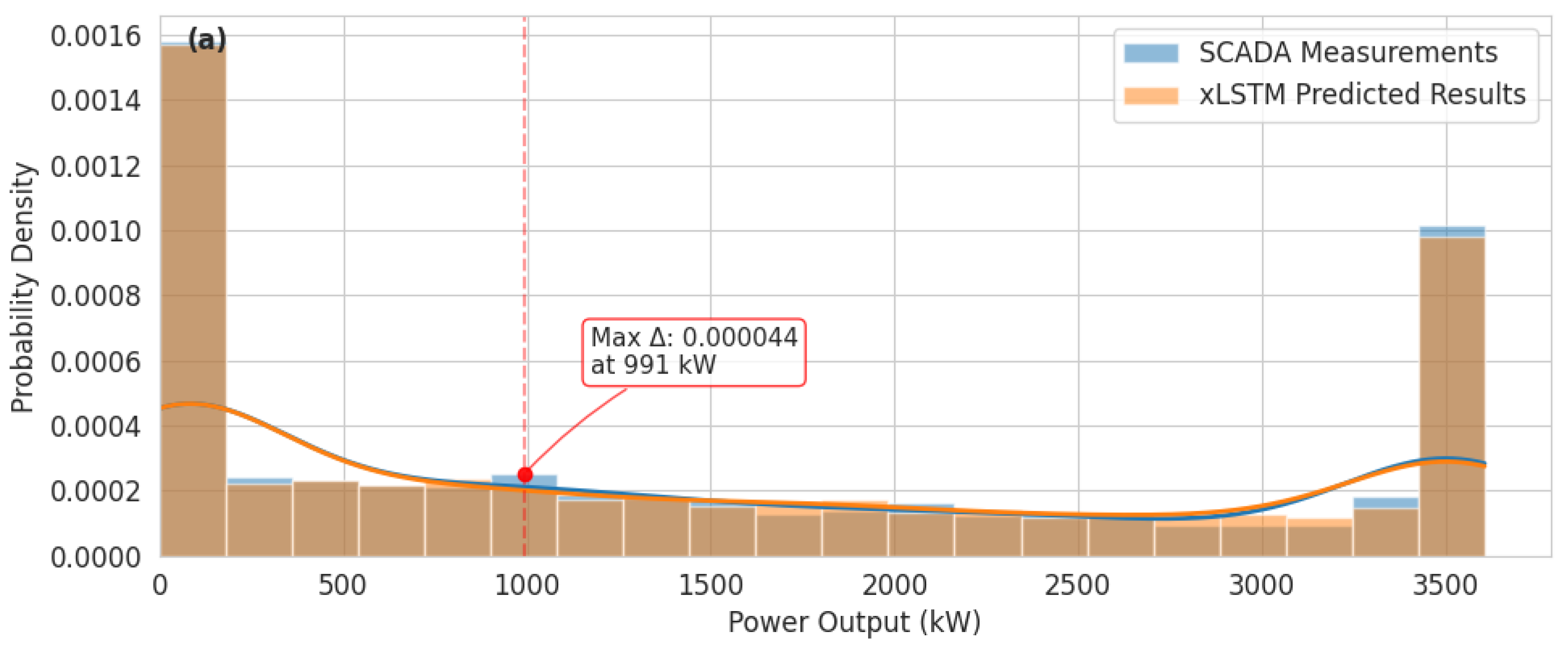
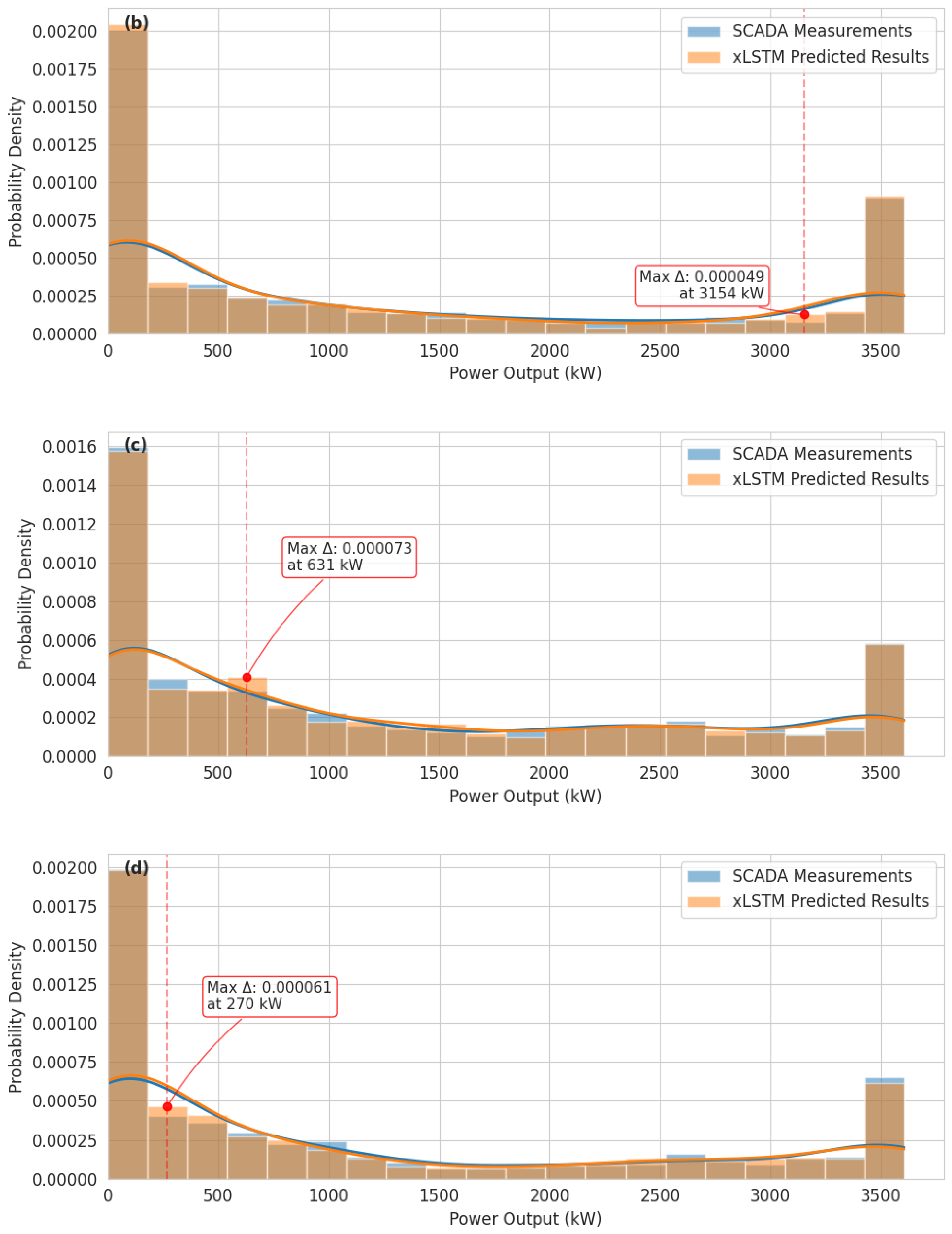
This study introduces a novel xLSTM architecture for wind power forecasting that addresses fundamental limitations in conventional recurrent neural networks. The xLSTM model’s key innovations, which are exponential gating with memory mixing and matrix memory structures, enable more effective processing of temporal dependencies in wind power data. Empirical evaluation using wind turbine SCADA data demonstrates the xLSTM model’s superior predictive performance across diverse operational conditions, achieving comprehensive metrics of R 2 = 0.923, MAPE ϵ = 8.47%, RMSE ξ = 34.6 kW, and MAE σ = 36.2 kW across all wind speed regimes.
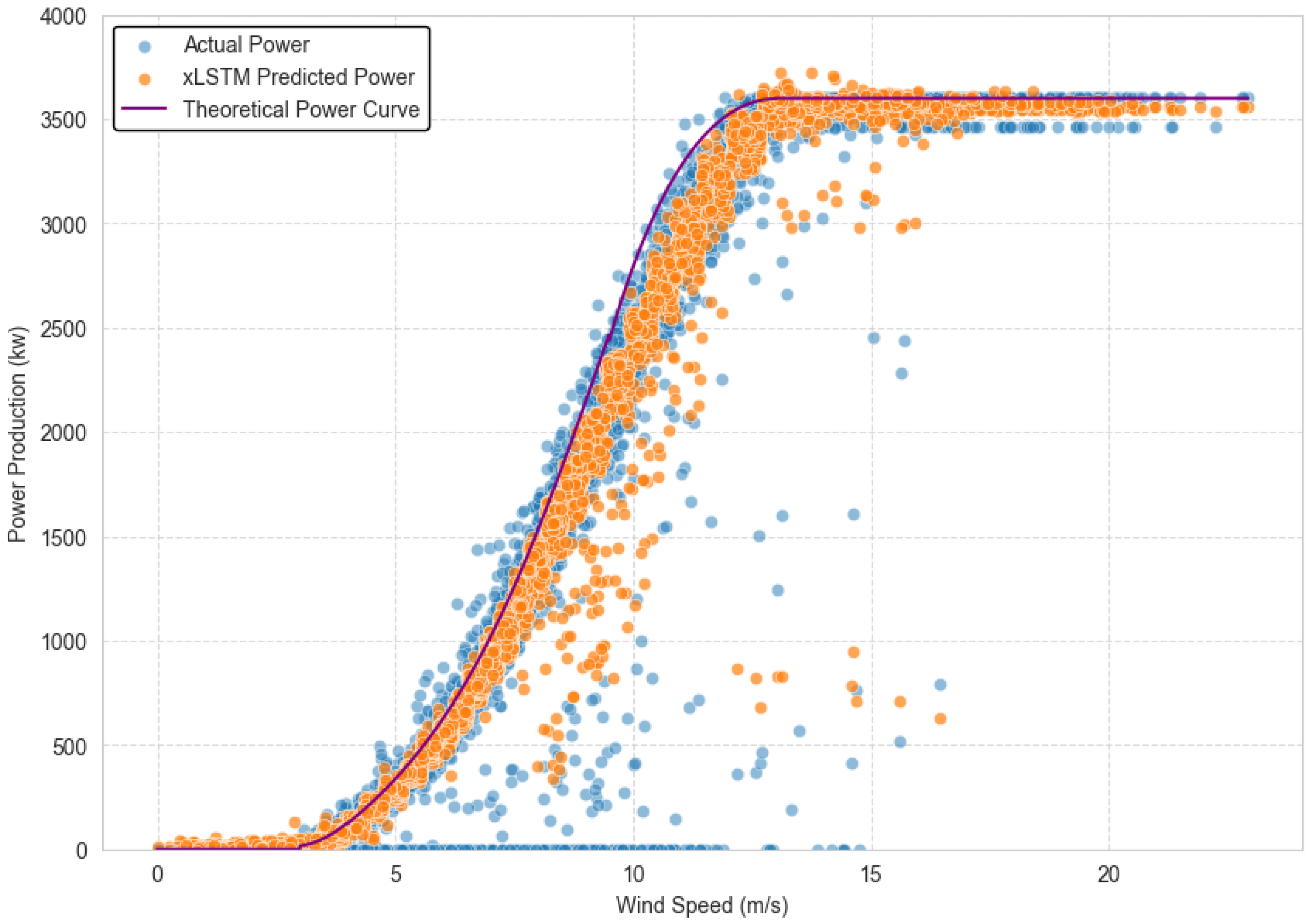
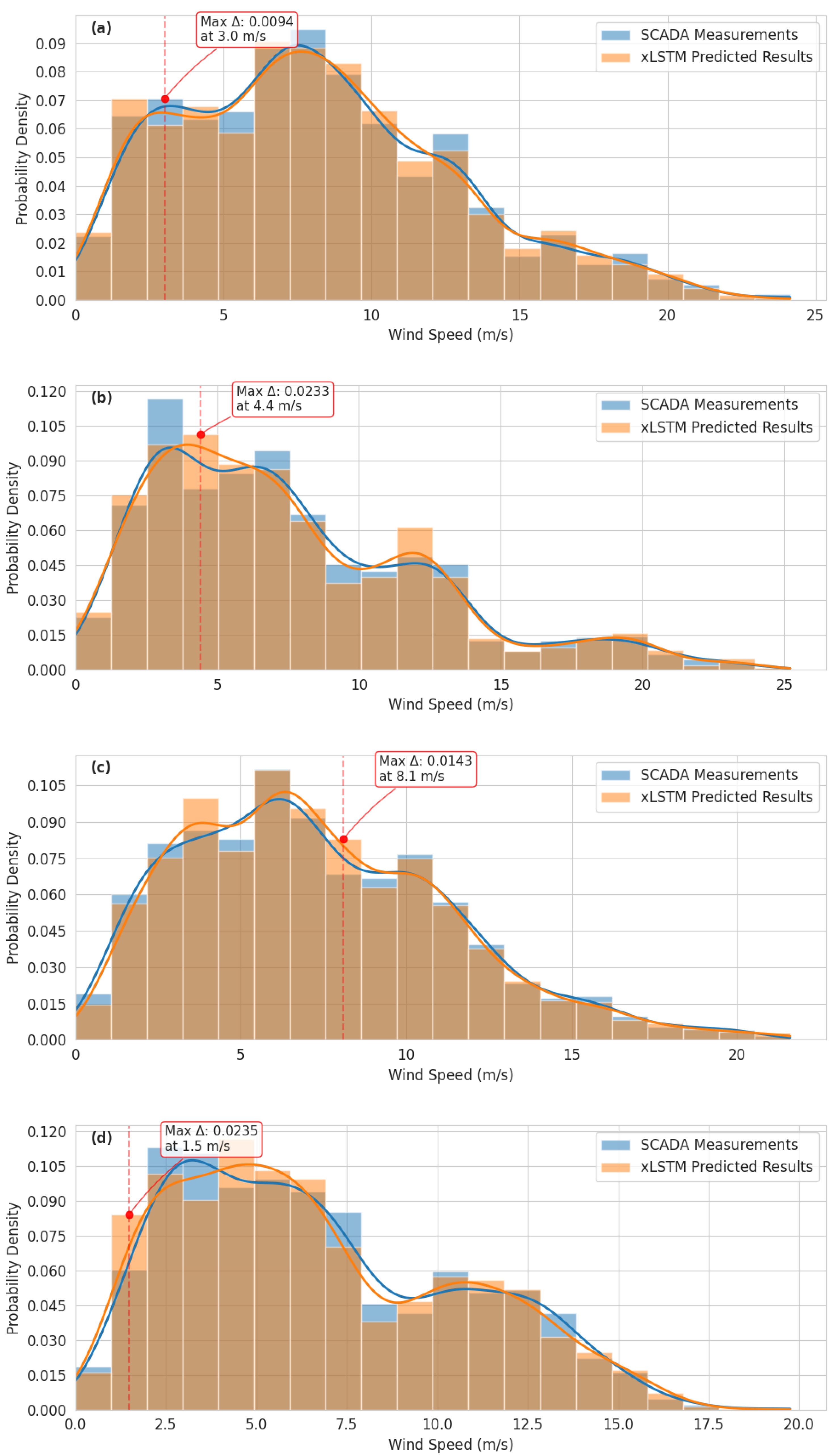
The xLSTM architecture demonstrates particularly strong performance in high wind speed conditions (>12 m/s), attaining an R 2 value of 0.954 and MAPE of 4.21%. This enhanced accuracy in the power curve’s plateau region provides significant value for operational planning and grid integration during periods of maximum generation. Seasonal analysis confirms the model’s robust temporal pattern recognition capabilities, with consistently strong predictive performance across all seasons ( R 2 values: 0.963–0.987) and effective modeling of both unimodal winter distributions and more complex bimodal patterns characteristic of transitional seasons.
The comparative analysis with established forecasting models demonstrates that xLSTM consistently outperforms traditional approaches like ARIMA (by 35.3%), standard recurrent architectures like LSTM and GRU (by approximately 6–7%), and even advanced models such as Transformers (by 2.3%) across all evaluation metrics. These quantitative improvements, particularly the 21.1% reduction in MAPE compared with conventional LSTM, validate the architectural enhancements of exponential gating and matrix memory structures as significant contributions to the field of wind power forecasting.
The architectural components work synergistically, with mLSTM enhancing parallel sequence processing and information flow while sLSTM with exponential gating enables more effective revision of stored information through scalar cell states. This complementary integration provides a robust framework for modeling the complex, non-linear relationships inherent in wind power generation. The xLSTM model demonstrates significant improvements over conventional approaches in computational efficiency, prediction accuracy, and generalizability across varying temporal and meteorological conditions.
Future work will address the limitations of our current study by expanding both the spatial and temporal dimensions of our analysis. Future work will extend the current forecasting framework of xLSTM to multiturbine wind farm settings, which will enable investigation of inter-turbine interactions, wake effects, and spatial dependencies that affect aggregate power generation. The xLSTM model’s temporal robustness will be enhanced through the incorporation of physics-based constraints and meteorological features that may improve long-term stability and performance under extreme weather conditions. Efficient transfer learning mechanisms will be developed to continuously update model parameters as new operational data becomes available, reducing the need for complete retraining while maintaining prediction accuracy across extended operational periods. The generalizability concerns identified in the current implementation will be collectively addressed by these developments while preserving the computational efficiency advantages of the xLSTM architecture.

Author Contributions

Conceptualization, Z.B. and G.L.; methodology, Z.B.; validation, Z.B. and G.L.; formal analysis, Z.B.; investigation, Z.B.; resources, G.L.; data curation, G.L.; writing—original draft preparation, Z.B.; writing—review and editing, G.L.; visualization, Z.B.; supervision, G.L.; project administration, G.L.; funding acquisition, G.L. All authors have read and agreed to the published version of the manuscript.

Funding

This research was funded by the U.S. National Science Foundation under Grant No. OIA-2429540.

Data Availability Statement

Data are contained within the article.

Conflicts of Interest

The authors declare no conflicts of interest.

References

  1. Sadorsky, P. Wind energy for sustainable development: Driving factors and future outlook. J. Clean. Prod. 2021, 289, 125779. [Google Scholar]
  2. Arockia Dhanraj, J.; Alkhawaldeh, R.S.; Van De, P.; Sugumaran, V.; Ali, N.; Lakshmaiya, N.; Chaurasiya, P.K.; Priyadharsini, S.; Velmurugan, K.; Chowdhury, M.S.; et al. Appraising machine learning classifiers for discriminating rotor condition in 50W–12V operational wind turbine for maximizing wind energy production through feature extraction and selection process. Front. Energy Res. 2022, 10, 925980. [Google Scholar]
  3. Blaabjerg, F.; Ma, K. Wind Energy Systems. Proc. IEEE 2017, 105, 2116–2131. [Google Scholar] [CrossRef]
  4. Magazzino, C.; Mele, M.; Schneider, N. A machine learning approach on the relationship among solar and wind energy production, coal consumption, GDP, and CO2 emissions. Renew. Energy 2021, 167, 99–115. [Google Scholar]
  5. Adeyeye, K.; Ijumba, N.; Colton, J. Exploring the environmental and economic impacts of wind energy: A cost-benefit perspective. Int. J. Sustain. Dev. World Ecol. 2020, 27, 718–731. [Google Scholar]
  6. Ma, Z.; Mei, G. A hybrid attention-based deep learning approach for wind power prediction. Appl. Energy 2022, 323, 119608. [Google Scholar] [CrossRef]
  7. Liu, X.; Cao, Z.; Zhang, Z. Short-term predictions of multiple wind turbine power outputs based on deep neural networks with transfer learning. Energy 2021, 217, 119356. [Google Scholar] [CrossRef]
  8. Cai, Y.; Bréon, F.M. Wind power potential and intermittency issues in the context of climate change. Energy Convers. Manag. 2021, 240, 114276. [Google Scholar]
  9. Wang, J.; Zhu, H.; Zhang, Y.; Cheng, F.; Zhou, C. A novel prediction model for wind power based on improved long short-term memory neural network. Energy 2023, 265, 126283. [Google Scholar]
  10. Chen, G.; Tang, B.; Zeng, X.; Zhou, P.; Kang, P.; Long, H. Short-term wind speed forecasting based on long short-term memory and improved BP neural network. Int. J. Electr. Power Energy Syst. 2022, 134, 107365. [Google Scholar]
  11. Farah, S.; David, A.W.; Humaira, N.; Aneela, Z.; Steffen, E. Short-term multi-hour ahead country-wide wind power prediction for Germany using gated recurrent unit deep learning. Renew. Sustain. Energy Rev. 2022, 167, 112700. [Google Scholar] [CrossRef]
  12. Alkesaiberi, A.; Harrou, F.; Sun, Y. Efficient wind power prediction using machine learning methods: A comparative study. Energies 2022, 15, 2327. [Google Scholar] [CrossRef]
  13. Liu, L.; Liu, J.; Ye, Y.; Liu, H.; Chen, K.; Li, D.; Dong, X.; Sun, M. Ultra-short-term wind power forecasting based on deep Bayesian model with uncertainty. Renew. Energy 2023, 205, 598–607. [Google Scholar] [CrossRef]
  14. Shahid, F.; Zameer, A.; Muneeb, M. A novel genetic LSTM model for wind power forecast. Energy 2021, 223, 120069. [Google Scholar] [CrossRef]
  15. Ahmad, T.; Zhang, D. A data-driven deep sequence-to-sequence long-short memory method along with a gated recurrent neural network for wind power forecasting. Energy 2022, 239, 122109. [Google Scholar] [CrossRef]
  16. Jiang, T.; Liu, Y. A short-term wind power prediction approach based on ensemble empirical mode decomposition and improved long short-term memory. Comput. Electr. Eng. 2023, 110, 108830. [Google Scholar] [CrossRef]
  17. Kisvari, A.; Lin, Z.; Liu, X. Wind power forecasting–A data-driven method along with gated recurrent neural network. Renew. Energy 2021, 163, 1895–1909. [Google Scholar] [CrossRef]
  18. Xiang, L.; Liu, J.; Yang, X.; Hu, A.; Su, H. Ultra-short term wind power prediction applying a novel model named SATCN-LSTM. Energy Convers. Manag. 2022, 252, 115036. [Google Scholar] [CrossRef]
  19. Yildiz, C.; Acikgoz, H.; Korkmaz, D.; Budak, U. An improved residual-based convolutional neural network for very short-term wind power forecasting. Energy Convers. Manag. 2021, 228, 113731. [Google Scholar] [CrossRef]
  20. Chen, Y.; Wang, Y.; Dong, Z.; Su, J.; Han, Z.; Zhou, D.; Zhao, Y.; Bao, Y. 2-D regional short-term wind speed forecast based on CNN-LSTM deep learning model. Energy Convers. Manag. 2021, 244, 114451. [Google Scholar] [CrossRef]
  21. Bazionis, I.K.; Georgilakis, P.S. Review of deterministic and probabilistic wind power forecasting: Models, methods, and future research. Electricity 2021, 2, 13–47. [Google Scholar] [CrossRef]
  22. Siami-Namini, S.; Tavakoli, N.; Namin, A.S. The performance of LSTM and BiLSTM in forecasting time series. In Proceedings of the 2019 IEEE International Conference on Big Data (Big Data), Los Angeles, CA, USA, 9–12 December 2019; pp. 3285–3292. [Google Scholar]
  23. Rezk, N.M.; Purnaprajna, M.; Nordström, T.; Ul-Abdin, Z. Recurrent neural networks: An embedded computing perspective. IEEE Access 2020, 8, 57967–57996. [Google Scholar]
  24. Moreno, S.R.; da Silva, R.G.; Mariani, V.C.; dos Santos Coelho, L. Multi-step wind speed forecasting based on hybrid multi-stage decomposition model and long short-term memory neural network. Energy Convers. Manag. 2020, 213, 112869. [Google Scholar]
  25. Nascimento, E.G.S.; de Melo, T.A.; Moreira, D.M. A transformer-based deep neural network with wavelet transform for forecasting wind speed and wind energy. Energy 2023, 278, 127678. [Google Scholar] [CrossRef]
  26. Qu, K.; Si, G.; Shan, Z.; Kong, X.; Yang, X. Short-term forecasting for multiple wind farms based on transformer model. Energy Rep. 2022, 8, 483–490. [Google Scholar]
  27. Wu, H.; Meng, K.; Fan, D.; Zhang, Z.; Liu, Q. Multistep short-term wind speed forecasting using transformer. Energy 2022, 261, 125231. [Google Scholar]
  28. Sun, S.; Liu, Y.; Li, Q.; Wang, T.; Chu, F. Short-term multi-step wind power forecasting based on spatio-temporal correlations and transformer neural networks. Energy Convers. Manag. 2023, 283, 116916. [Google Scholar] [CrossRef]
  29. Xiang, L.; Fu, X.; Yao, Q.; Zhu, G.; Hu, A. A novel model for ultra-short term wind power prediction based on Vision Transformer. Energy 2024, 294, 130854. [Google Scholar]
  30. Lindemann, B.; Müller, T.; Vietz, H.; Jazdi, N.; Weyrich, M. A survey on long short-term memory networks for time series prediction. Procedia Cirp 2021, 99, 650–655. [Google Scholar] [CrossRef]
  31. Li, G.; Wu, Y.; Yesha, Y. Decentralized condition monitoring for distributed wind systems: A federated learning-based approach to enhance SCADA data privacy. In Proceedings of the ASME 2024 18th International Conference on Energy Sustainability (ES2024), Anaheim, CA, USA, 15–17 July 2024; p. V001T01A010. [Google Scholar]
Figure 1. Polar coordinate distribution for wind speeds and wind directions.
Algorithms 18 00206 g001
Figure 2. Comparison of theoretical, actual, and xLSTM predicted power output of the wind turbine.
Algorithms 18 00206 g002
Figure 3. Seasonal probabilistic distribution of wind speeds: comparative analysis of SCADA measurements and xLSTM predictions in (a) winter (December–February), (b) spring (March–May), (c) summer (June–August), and (d) autumn (September–November).
Algorithms 18 00206 g003
Figure 4. Seasonal probabilistic distribution of power generation characteristics: comparative analysis of SCADA measurements and xLSTM predictions in (a) winter (December–February), (b) spring (March–May), (c) summer (June–August), and (d) autumn (September–November).
Algorithms 18 00206 g004aAlgorithms 18 00206 g004b
Table 1. Raw SCADA data for wind power output prediction of a wind turbine [31].
Date and TimeWind Speed (m/s)Wind Direction (°)Rotor Speed (rpm)Yaw Angle (°)Actual Power (kW)
1 January 2021 0:005.20465304.8330313.3650
1 January 2021 0:105.85888299.3380313.3650
1 January 2021 0:206.06903299.1730313.3650
1 January 2021 0:305.91886296.6470313.3650
1 January 2021 0:405.40831291.8270313.3650
1 January 2021 0:505.58617287.7160313.3650
1 January 2021 1:005.62896289.5370313.3650
31 December 2021 23:008.6017035.80314.90336.7802449.45
31 December 2021 23:109.0781638.17915.01336.7802451.86
31 December 2021 23:209.1197144.45214.96836.7802361.74
31 December 2021 23:308.9195140.383415.01336.7802298.64
31 December 2021 23:409.5568944.21414.96636.7802361.43
31 December 2021 23:5010.0656841.61315.16037.9873795.41
Table 2. Distribution of SCADA data by wind direction ranges.
Wind Direction RangeRaw DataOutliersRemaining Data
0 45 63144015913
45 90 58523725480
90 135 47953054490
135 180 51033244779
180 225 71284536675
225 270 85465438003
270 315 79325047428
315 360 48603124548
Total50,530321447,316
Table 3. Hyperparameter Configuration for sLSTM.
ParameterValueDescription
Input Size1Dimension of input features
Head Size32Dimension per attention head
Number of Heads4Parallel attention mechanisms
Projection Factor4/3Feed-forward network expansion ratio
Forget Gate Init[3, 6]Initialization range for forget gates
Batch Size32Training batch size
Learning Rate0.01Initial learning rate for optimization
Table 4. Hyperparameter Configuration for mLSTM.
ParameterValueDescription
Input Size1Dimension of input features
Head Size32Dimension per attention head
Number of Heads4Parallel attention mechanisms
Projection Factor2.0Matrix memory expansion ratio
Matrix Memory Dim128Dimension of matrix memory
Batch Size32Training batch size
Learning Rate0.01Initial learning rate for optimization
Table 5. Performance metrics of xLSTM model for wind power prediction.
Wind Speed RangeR2MAPE ϵ (%)RMSE ξ (kW)MAE σ (kW)
Low (0–5 m/s)0.8869.6532.729.4
Medium (5–12 m/s)0.90111.8335.547.8
High (>12 m/s)0.9544.2134.242.6
Overall0.9238.4734.636.2
Table 6. Comparison of seasonal probabilistic distribution between SCADA measurements with xLSTM predictions of wind speeds.
Statistical ParameterWinterSpringSummerAutumn
SCADAxLSTMSCADAxLSTMSCADAxLSTMSCADAxLSTM
Central Tendency
Primary Mode (m/s)7.87.53.43.66.46.53.54.8
Secondary Mode (m/s)8.28.810.810.5
Mean Wind Speed (m/s)8.28.16.97.17.37.16.46.5
Median Wind Speed (m/s)7.57.45.86.26.86.75.75.9
Distribution Shape
Standard Deviation (m/s)4.84.65.15.34.34.24.34.5
Coefficient of Variation0.580.570.740.750.590.590.670.69
Skewness0.670.640.780.740.590.560.420.39
Kurtosis2.872.912.712.652.592.632.652.72
Bimodality Coefficient0.420.410.590.560.470.450.530.51
Distribution Entropy (bits)2.672.702.762.792.742.722.832.81
Probability Characteristics
Prob. Density at Primary Mode0.0920.0880.1160.0950.0990.1020.1060.104
Prob. Density at Secondary Mode0.0450.0610.0550.052
Prob. Wind Speed < 5 m/s0.270.260.420.380.310.330.380.41
Prob. Wind Speed > 12 m/s0.220.210.190.200.180.170.160.15
Error Metrics
MAPE in Probability Density (%)4.38.75.27.1
RMSE0.0240.0380.0290.035
R 2 0.9870.9630.9780.971
Table 7. Comparison of seasonal probabilistic distribution metrics for power output between SCADA measurements and xLSTM predictions.
Statistical ParameterWinterSpringSummerAutumn
SCADAxLSTMSCADAxLSTMSCADAxLSTMSCADAxLSTM
Central Tendency
Primary Mode (kW)00000000
Secondary Mode (kW)35003500350035003500350035003500
Mean Power (kW)14851523132613751297134211861232
Median Power (kW)876907742788823865693745
Distribution Shape
Standard Deviation (kW)13561387128713151183120511641189
Coefficient of Variation0.9130.9110.9710.9560.9120.8980.9820.965
Skewness0.6320.6080.7450.7260.5870.5760.8240.793
Kurtosis1.8431.8141.9631.9381.7421.7262.1032.072
Bimodality Coefficient0.5670.5610.5940.5860.5230.5170.6210.612
Probability Characteristics
Prob. Density at Primary Mode ( × 10 4 )2.204.203.505.803.805.606.506.70
Prob. Density at Secondary Mode ( × 10 4 )10.209.409.208.405.906.306.502.30
Prob. Power < 500 kW0.2640.2430.3170.2860.2860.2670.3440.316
Prob. Power > 3000 kW0.1870.1960.1630.1720.1380.1450.1240.137
Error Metrics
MAPE in Probability Density (%)5.827.436.158.76
RMSE (kW)143.6168.2152.8187.3
R 2 0.9820.9730.9780.967
Table 8. Computational performance comparison between xLSTM and baseline models.
ModelTraining Time (min) 1Inference Time (ms/Sample)Memory Usage (MB)Scalability Factor
LSTM4.23.51861.00
xLSTM [0:1]5.14.22141.22
xLSTM [1:0]5.64.82371.28
xLSTM [7:1]5.44.62281.25
1 Training time measured on a system with NVIDIA RTX 4090 GPU for 50 epochs with batch size 32.
Table 9. Performance comparison of xLSTM against benchmark forecasting models.
ModelOverall R 2 MAPE ϵ (%)RMSE ξ (kW)Low Wind R 2 Medium Wind R 2 High Wind R 2 Training Time (min)
ARIMA0.68217.3563.70.5840.6930.7120.5
LSTM0.86411.2342.30.8010.8450.8923.8
GRU0.87110.9541.50.8130.8510.8973.5
BiLSTM0.88510.2138.90.8260.8640.9174.6
Transformer0.9029.3736.10.8350.8860.9367.2
xLSTM0.9238.4734.60.8860.9010.9545.4
Disclaimer/Publisher’s Note: The statements, opinions and data contained in all publications are solely those of the individual author(s) and contributor(s) and not of MDPI and/or the editor(s). MDPI and/or the editor(s) disclaim responsibility for any injury to people or property resulting from any ideas, methods, instructions or products referred to in the content.

