A Two-Stage Multi-Objective Optimization Algorithm for Solving Large-Scale Optimization Problems

Abstract

For large-scale multi-objective optimization, it is particularly challenging for evolutionary algorithms to converge to the Pareto Front. Most existing multi-objective evolutionary algorithms (MOEAs) handle convergence and diversity in a mutually dependent manner during the evolution process. In this case, the performance degradation of one solution may lead to the deterioration of the performance of the other solution. This paper proposes a two-stage multi-objective optimization algorithm based on decision variable clustering (LSMOEA-VT) to solve large-scale optimization problems. In LSMOEA-VT, decision variables are divided into two categories and use dimensionality reduction methods to optimize the variables that affect evolutionary convergence. Following this, we performed an interdependence analysis to break down the convergence variables into multiple subcomponents that are more tractable. Furthermore, a non-dominated dynamic weight aggregation method is used to enhance the diversity of the population. To evaluate the performance of our proposed algorithm, we performed extensive comparative experiments against four optimization algorithms across a diverse set of benchmark problems, including eight multi-objective optimization problems and nine large-scale optimization problems. The experimental results show that our proposed algorithm performs well on some test functions and has certain competitiveness.

1. Introduction

In the field of evolutionary computation, researchers only focus on single-objective optimization problems; however, as real-world problems grow in complexity, they frequently involve multiple conflicting objectives, leading to their classification as multi-objective optimization problems (MOPs). To tackle these challenges, scholars have developed a plethora of evolutionary algorithms, such as NSGA-II [1], MOEA/D [2], and NSGA-III [3].

Empirical evidence demonstrates that these algorithms have yielded commendable outcomes in both benchmark scenarios and practical applications [4,5,6]. However, due to the increasing complexity of problems in the real world, such as engineering design [7], traffic control [8], and groundwater monitoring [9]. Numerous problems encompass a vast array of decision variables, and due to the curse of dimensionality, the efficacy and efficiency of prevailing optimization methodologies experience a significant decline as the dimensionality escalates. Generally speaking, there are two reasons for this phenomenon: convergence pressure and diversity management. The former issue arises from the fact that in multi-objective optimization, as the number of decision variables grows, the solution space volume increases at an exponential rate, leading to a dramatic increase in computational complexity. The latter challenge stems from the sparse distribution of candidate solutions within the objective space, which undermines the efficacy of conventional diversity maintenance strategies.

To address this category of problems, a “divide and conquer” strategy is commonly employed, which was first proposed in [10]. The core concept involves partitioning the large-scale decision variables in large-scale multi-objective problems (LSMOPs) into multiple lower-dimensional groups and subsequently optimizing each sub-problem independently following decomposition.

In the context of coevolution, the selection of an appropriate decomposition strategy is of paramount importance. The most optimal strategy entails grouping variables that exhibit interactions while segregating independent variables into distinct groups. Currently, there are two predominant grouping strategies: one is the fixed grouping strategy [11,12,13], and the other is the dynamic grouping strategy [14,15]. In a fixed grouping strategy, the composition of groups remains unchanged throughout the optimization process, as exemplified by the LMEA [16]. Conversely, in dynamic grouping strategies, the grouping configuration evolves continuously in tandem with the optimization process, as seen in the CCGDE3. The efficacy of grouping decision variables significantly influences the performance of the algorithm. For single-objective optimization problems [17,18], due to the straightforward dependency relationships among variables, such issues are relatively more tractable. In contrast, multi-objective problems involve intricate dependencies [19,20,21] not only among variables but also across multiple objectives, thereby compounding the complexity of the solution process. Consequently, the judicious grouping of decision variables presents a formidable challenge.

When addressing multi-objective optimization problems, it is imperative to account for the interrelationships among variables. Researchers have undertaken extensive work in this domain, with two of the most seminal algorithms being the multi-objective evolutionary algorithm based on decision variable analysis (MOEA/DVA) [22] and the evolutionary algorithm based on decision variable clustering (LMEA) [16]. Both algorithms categorize decision variables into convergence variables and diversity variables. Convergence variables are associated with the proximity of the population to the true Pareto front, whereas diversity variables govern the distribution of the population within the objective space.

This paper proposes a two-stage large-scale optimization algorithm based on clustering for large-scale multi-objective optimization problems. The main contributions are summarized as follows.

(1)

The decision variable clustering strategy effectively categorizes all variables into two distinct groups: those related to diversity and those related to convergence, thereby facilitating the evolutionary process. This approach employs the angle between the convergence direction and the sampled solution as a distinguishing feature, subsequently clustering these features using the k-means method. Variables associated with smaller angles contribute more significantly to convergence, whereas those with larger angles play a more substantial role in enhancing diversity.

(2)

By employing the non-dominated dynamic weight aggregation method, Pareto optimal solutions are identified in multi-objective optimization problems (MOPs) with varying Pareto front shapes. Subsequently, the optimization problem involving reference lines is addressed by leveraging these solutions within the Pareto optimal subspace, thereby resolving the population diversity issue.

(3)

To assess the efficacy of the proposed algorithm, comprehensive empirical evaluations were performed on a range of benchmark problems. These evaluations involved comparisons with several advanced MOEAs designed for addressing both multi-objective optimization problems and large-scale optimization challenges. The experimental results conclusively demonstrate that the algorithm introduced in this study is capable of effectively solving large-scale optimization problems characterized by numerous decision variables, achieving commendable performance outcomes.

In the latter half of the article, we first reviewed the relevant concepts in Section 2. The Section 3 introduces some details of the main process of the proposed algorithm. The Section 4 is related experiments and results. The Section 5 is the conclusion and outlook for future work.

2. Background

2.1. Multi-Objective Optimization

Optimization problems with multiple mutually conflicting objectives are called MOPs. A MOP can be described by Equation (1), where $x=\left(x_1,x_2,\dots ,x_D\right)$ represents a candidate solution and D is the dimension of the decision vector. M is the dimension of the target space, which is the number of targets in MOP. When D ≥ 100, MOP is considered a large-scale multi-objective optimization problem.

$$\left\{\begin{array}{c}\min F\left(x\right)=\left\{f_1\left(x\right),f_2\left(x\right),\dots ,f_M\left(x\right)\right\}\\ subject to:x\in {\mathsf{\Omega }}^D\end{array}\right.$$

(1)

In multi-objective optimization problems, there are a large number of optimal solutions that cannot be mutually dominated. Assuming there are two candidate solutions $x_1$ and $x_2$ in the decision space ${\mathsf{\Omega }}^D$. When they satisfy Equation (2), $x_1$ Pareto dominates $x_2$, denoted as $x_1\prec x_2$. We can define the dominance relationship between the two solutions of the minimum MOP as follows:

$$\left\{\begin{array}{c}\forall i=\mathrm{1,2},\dots ,M, f_i\left(x_1\right)\le f_i\left(x_2 \right)\\ \exists j=\mathrm{1,2},\dots ,M, f_j\left(x_1\right)<f_j\left(x_2 \right)\end{array}\right.$$

(2)

Generally speaking, it is difficult to obtain all Pareto optimal solutions. Therefore, we achieve three goals: (1) Enhance the convergence ability of the algorithm so that all final solutions are close to the true Pareto front (PF). (2) Improve the diversity of algorithms so that the target vector has a diverse distribution on the PF while satisfying the convergence speed condition; (3) Minimize the waste of computing resources while ensuring convergence and diversity. In the past few years, the field of multi-objective optimization has attracted a lot of attention, and many researchers are dedicated to the research in this area.

2.2. Large-Scale Multi-Objective Optimization

In practical applications, there are a large number of multi-objective optimization problems containing thousands of decision variables, but existing multi-objective evolutionary algorithms cannot perfectly solve these problems. Experience has shown that as the number of variables in the search space increases, the effectiveness of most MOEAs sharply decreases. In LSMOEAs based on decision variable grouping, the result of decision variable grouping will directly affect the final solution quality. Although the existing algorithms can achieve satisfactory results in most cases, there will be a lack of diversity of solutions for some problems. As shown in Figure 1, the black curve represents the ideal Pareto frontier for the bi-objective optimization problem BT6, and the gray point represents the feasible solution obtained by the algorithm in the current optimization stage. It can be seen from Figure 1 that as the algorithm evolves, the solution obtained gradually concentrates on a local point on the Pareto front. This shows that with the evolution of the algorithm, the diversity of the population has been significantly lost. Paper [15] first applied the coevolution (CC) framework to evolutionary algorithms for solving large-scale multi-objective optimization problems. Recently, Ma et al. proposed a multi-objective evolutionary algorithm for solving large-scale multi-objective problems, called MOEA/DVA [22]. The algorithm uses a method called decision variable analysis to divide all decision variables into three categories. By perturbing the value of some variables, if the generated solution is not dominant after the variable perturbation and is not dominated by other solutions, the variable is called a distance variable. If there is a dominant relationship between the solutions generated after the disturbance, this variable is called the position variable. Otherwise, this variable is called a mixed variable. Zhang [16] proposed another new evolutionary algorithm using the decision variable clustering method. It first clusters all decision variables into two categories, one of which affects the convergence performance, and the other variables are related to diversity. Then in the optimization process, two different strategies are adopted for the two categories.

In addition, there is a dynamic grouping strategy. In the paper [23], Wolfe first designed a decomposition pool with different group sizes. Then, select one of the group sizes from the pool. Divides the entire dimension into many groups of different sizes based on the selected grouping size. This method can save a lot of computing resources. In addition, another strategy is to transform the original LSMOP into a simpler MOP with a relatively small number of decision variables. The weighted optimization framework (WOF) [24] is representative of this category. In WOF, decision variables are divided into several groups, each of which has a weight variable. Therefore, the optimization of the same group of weight variables can be regarded as the optimization of the subproblem in the original decision space subspace. Another typical algorithm is a large-scale multi-objective algorithm based on problem reconstruction (LSMOF) [25]. The core idea of LSMOF is to transform the original LSMOP into a low-dimensional single-objective optimization problem through problem reconstruction. In the reconstructed problem, the decision space is reduced from the dimension of weight variable reconstruction, and the target space is therefore reduced, so a group of excellent solutions can be obtained efficiently.

There are also some other strategies, such as the recently proposed multi-objective particle swarm optimization algorithm based on the competition mechanism (CMOPSO) [26], which does not use a grouping strategy or decision variable analysis strategy but uses a particle swarm optimizer (PSO) to enhance the diversity of the population and uses a paired competition strategy [27] to solve LSMOP. Zhang et al. [28] established an information feedback model (IFM) to generate promising population offspring. IM-MOEA [29] built an inverse model based on a Gaussian process, mapping the solution from the target space to the decision space so as to generate children by sampling the target space.

3. Proposed Algorithm

In this section, we proposed a two-stage large-scale optimization algorithm based on decision variable clustering to solve large-scale multi-objective optimization problems, named LSMOEA-VT. The main framework of LSMOEA-VT was shown in Algorithm 1.

Algorithm 1 Main Framework of LSMOEA-VT

Input: N (population size), nSel (number of selected solutions for decision variable clustering), nPer (number of perturbations on each solution for decision variable clustering), nCor (number of selected solutions for decision variable interaction analysis) a set of uniformly distributed reference lines $\mathrm{r}=\left\{r_1,r_2,\dots ,r_n\right\}$. Output: P (final population)

1. P ← Initialize(N);

2. [DV, CV] ← VariableClustering (P, nSel, nPer);

3. subCVs ←InteractionAnalysis (P, CV, nCor);

4. while termination criterion not fulfilled do

5.   P′ ← ConvergenceOptimization(P, subCVs);

6.   Q ← Find some Pareto-optimal solutions of $f\left(x\right)$

7.   Ω ← Learn the subspace based on Q;

8.   Update the given reference lines $r=\left\{r_1,r_2,\dots ,r_n\right\}$;

9.   P ← Diversity maintaining with $r$ in Ω;

10. Return P.

In the first stage of the algorithm, we use clustering methods to divide all decision variables into two categories, one related to convergence and the other related to diversity. Therefore, we can apply specific treatments to each group. Due to the fact that the number of decision variables after clustering may still be relatively large, we can conduct interdependence analysis on these variables to test the interdependence relationships between them. In the second stage, we can search for a set of Pareto optimal solutions for a given large-scale problem, then learn POS from the found Pareto optimal solutions, and finally obtain a final solution with convergence and diversity by updating the given reference line. Several crucial components of LSMOEA-VT are further illustrated in the coming parts.

3.1. Clustering of Decision Variables

Algorithm 2 delineates the methodology for clustering decision variables. Consider a bi-objective optimization problem wherein each individual comprises five decision variables, denoted as x₁, x₂, x₃, x₄, and x₅. Firstly, two candidate solutions are randomly selected from the entire solution set. Subsequently, the variables of these selected solutions are perturbed ten times. The perturbed solutions are then normalized to form a fitting line, denoted as L. The equation f₁ + ⋯ + f_m = 1 represents the direction of convergence. In high-dimensional decision spaces, dynamic clustering during optimization would introduce significant computational overhead, especially when evaluating complex objective functions. Offline clustering allows us to preprocess the decision space and reduce computational complexity during the optimization process; clustering provided a stable and consistent framework for interaction analysis. Dynamic clustering, while potentially more adaptive, could introduce variability in the sensitivity analysis due to changes in cluster boundaries during optimization. By performing clustering offline, we establish a fixed reference framework that facilitates clearer interpretation of the relationships between decision variables and objective functions. Following this, the angle between the fitting line L and the hyperplane normal is calculated. Variables exhibiting larger angles contribute more significantly to diversity, whereas those with smaller angles contribute more to convergence. It is noteworthy that the greater the number of candidate solutions selected for decision variables, the more angles associated with each variable will be generated. Therefore, to achieve more precise results, it is advisable to select as many solutions as feasible. Finally, the k-means clustering method is employed to partition all variables in the decision space into two groups. Variables with smaller average angles are categorized as convergence-related variables, while the remaining variables are classified as diversity-related variables.

Algorithm 2 Clustering of Decision Variables
Input: pop, number of candidate solutionsSelNum, number of perturbationPerNum Output: [Diver,Conver]
1.	for i = 1:n do
2.	C ← Choose SelNum solutions from pop randomly;
3.	for j = 1:SelNum do
4.	Make perturbation for the i-th variable of C[j] for PerNum times to bring a generation SP and then normalize it;
5.	Generate a line L for SP in objective space;
6.	Angle[i][j] ← the angle between L and normal line of hyperplane;
7.	MSE[i][j] ← the mean square error of the fitting;
8.	end for
9.	end for
10.	CV ← {mean(MSE[i]) < 1 × 10−2};
11.	[C1, C2] ← apply k-means to group all variables into two categories adopting Angle as feature;
12.	if CV⋂C1 ≠ ∅ and CV⋂C2 ≠ ∅ then
13.	CV ← CV⋂C, C is either C1 or C2 depending on which of the average of Angle is smaller;
14.	end if
15.	DV ← {j ∉ CV }

3.2. Interaction Analysis

The number of decision variables is very large in the large-scale optimization algorithm, and it will affect the convergence rate of real PF. Therefore, the interaction between convergence variables is tested in Algorithm 3. According to this relationship, these variables will continue to be divided into subgroups. The interacting variables are in the same subgroup, and there is no interaction between the two subgroups. Usually, the interaction between two variables is defined as ${\left.f\left(x\right)\right|}_{x_i=a_2,x_j=b_1}\triangleq f\left(x_1,\dots ,x_{i-1},a_2,\dots ,x_{j-1},b_1,\dots ,x_D\right).$ In brief, when the dominance relationship of the solution changes x_i and x_j. Respectively, the opposite results are produced; then, this pair of decision variables is dependent. In Algorithm 3, we first initialize the empty subset of the interaction variable group and then assign the convergence-related variables to different subgroups according to the paired interactions between variables. In extreme cases, there are two cases. One is that there is only one subgroup, which means that all convergence variables are completely separable. In the other case, if the decision variables are completely separable, the number of subgroups will be |CV|.

Algorithm 3 Interaction Analysis

Input: pop, Conver, number of chosen solutions CorNum Output: subCVs

1. set subCVs as ∅;

2. for all the ν ∈ CV do

3. set CorSet as ∅;

4.  for all the Group ∈ subCVs do

5.   for all the u ∈ Group do

6.    flag ← False;

7.    for i = 1: CorNum do

8.      Choose an individual p from pop randomly;

9.      if ν has interaction with u in individual p then

10.     flag ← True;

11.     CorSet = {Group} cupCorSet;

12.     Break;

13.    end if

14.    end for

15.    if flag is True then

16. Break;

17. end if

18. end for

19. end for

20. if CorSet = ∅ then

21. subCVs = subCVs∪{{ν}};

22. else

23. subCVs = subCVs/CorSet;

24. Group ← all variables in CorSet and ν;

25. subCVs = subCVs∪{Group};

26. end if

27. end for

3.3. Pareto Optimal Subspace Learning

Algorithm 4 represents the process of Pareto optimal subspace learning. First, the Pareto optimal solution in Q is represented by the matrix M ∈ R^|P|×n, and then M is updated to M′ (line 2 and line 3) by calculating the average value of M and subtracting the average value. Then, calculating the eigenvalues $\left[v_1,v_2,\dots ,v_n\right]$ of the M′ covariance matrix (line 4). Then calculate the median of each column in M (line 10) and set the elements in the lower and upper limits of x to the corresponding median. Finally, PoS is generated by sampling all points in the updated upper and lower limits (line 15).

Algorithm 4 Pareto-Optimal Subspace Learning
1.	Input: The Pareto-optimal solutions Q, a threshold value ε, the lower bound $\mathrm{l}\text{\_}\mathrm{l}\mathrm{i}\mathrm{m}\mathrm{i}\mathrm{t}$ = $\left[l_1,l_2,\dots l_n\right]$, the upper bound $\mathrm{u}\text{\_}\mathrm{l}\mathrm{i}\mathrm{m}\mathrm{i}\mathrm{t}$ = $\left[u_1,u_2,\dots u_n\right]$. Output: The learned Pareto-optimal subspace Ω
2.	Let a matrix M ∈ R|P|×n denote the solutions in Q
3.	mean ← Calculate the mean values of M;
4.	M′ ← Update M by subtracting mean;
5.	$\left[v_1,v_2,\dots ,v_n\right]$ ← Calculate the eigenvalues of the covariance matrix of M′;
6.	$\left[{ind}_1,{ind}_2,\dots ,{ind}_n\right]$ ← Record the positions of the eigenvalues with the descending order;
7.	$\mathrm{j}\leftarrow 0;$
8	While ${\sum }_{i=1}^{{ind}_j}{v}_i/{\sum }_{i=1}^n{v}_i$< ε do
9.	$j\leftarrow j+1;$
10.	end
11.	median ← Calculate the median value of each column in M;
12.	for i ← j + 1 to n do
13.	$l\text{\_}i$ ← Copy the ${ind}_i$ component of median;
14.	$u\text{\_}i$ ← Copy the ${ind}_i$ component of median;
15.	end
16.	Ω ← All points in $[l\text{\_}limit,u\text{\_}limit]$;
17.	Return Ω.

3.4. Maintaining Population Diversity

Algorithm 5 shows the detailed steps to maintain population diversity. First, we can draw the reference line by finding the extreme point, the lowest point, and the ideal point (lines 1–6, 7–12, and 13–15 of the algorithm). When searching for extreme points, each extreme point is obtained by processing the single objective problem in Ω; the definition is shown in Equation (3):

$$\left\{\begin{array}{c}maximize {\displaystyle \frac{{\sum }_{i=1}^m{f}_i(x)s_i}{\sqrt{{\sum }_{i=1}^m{f}_i^2(x)}\sqrt{{\sum }_{i=1}^m{s}_i^2}}} \\ s.t. x\in \Omega \end{array}\right.$$

(3)

In short, we can find the nearest solution of the angle between the target vector and the corresponding axis. In addition, the lowest point and ideal point are obtained by extracting the maximum and minimum values from each dimension of the extreme point, and the mapping of each reference line is realized by line 14 in the algorithm. The PF in the multi-objective optimization problem may not occupy the entire target space, or only a part of N reference lines pass through the PF. In this case, the final solution will lose diversity. Therefore, the purpose of drawing reference lines is to keep the preset N reference lines within PF as far as possible so as to maintain the diversity of solutions. Finally, each solution is obtained by solving SOP (4) with a set of reference lines r, and the reference lines in r are evenly distributed in PF, and each solution in Q has the smallest cosine value for each reference line, so the solution obtained has good diversity.

Algorithm 5 Diversity Maintaining
Input: The Pareto-optimal subspace Ω, the updated reference lines $\mathrm{r}=\left\{r_1,r_2,\dots ,r_n\right\}$; Output: P
1.	$extreme\text{\_}points$ ← ∅
2.	for i ← 1 to m do
3.	$\mathrm{s}=\left[s_1,s_2,\dots ,s_m\right]=\left[0,\dots 1,\dots ,0\right]$ ← Initialize a vector of m elements with zeros except for the i-th element with one;
4.	$x^{\ast }$ ← Solve the single-objective optimization problem
5.	$extreme\text{\_}points\leftarrow extreme\text{\_}points\cup f\left(x^{\ast }\right)$;
6.	end
7.	${nadir}_{\text{\_}}point$ ← ∅
8.	${ideal}_{\text{\_}}point$ ← ∅
9.	for i ← 1 to m do
10.	${nadir}_{\text{\_}}point$ ← ${nadir}_{\text{\_}}point\cup$The maximal element at the i-th component of $extreme\text{\_}points$;
11.	${ideal}_{\text{\_}}point$ ← ${ideal}_{\text{\_}}point\cup$The minimal element at the i-th component of $extreme\text{\_}points$;
12.	end
13.	for each$r\mathrm{in} r=\left\{r_1,r_2,\dots ,r_n\right\}$ do
14.	r ←  $r\times \left({nadir}_{\text{\_}}point-{ideal}_{\text{\_}}point\right)+{ideal}_{\text{\_}}point;$
15.	end
16.	P ← ∅
17.	for i ← 1 to N do
18.	$\mathrm{s}\leftarrow r_i$;
19.	P ← P∪$x^{\ast }$;
20.	end
21.	Return P.

4. Experiments and Results

In order to verify the effectiveness of the proposed algorithm, we compare it with four other advanced algorithms, namely NSGA-III [3], MOEA/D [2], MOEA/DVA [22], and LMEA [16]. on some standard test suits, namely DTLZ [30], WFG [31], UF [32], and LSMOP [33]. All experiments in this paper were run in MATLAB R2020b on a personal computer. The Windows 10 64-bit system is configured with an Intel (R) Core (TM) i7 4720HQ CPU and 12G of RAM. The computer is manufactured by ASUS in Suzhou, China.

4.1. Experimental Setting

For a fair comparison, all comparison algorithms use the recommended parameter values to achieve the best performance. The parameters of the experiment are set as follows: All comparison algorithms simulate binary crossover and polynomial mutation operations to generate offspring. For each test problem, the crossover probability is p_c = 1.0. Crossover probability is an important parameter in genetic algorithms used to control the probability of individuals performing crossover operations during the evolutionary process. The Pc is a value between 0 and 1, representing the probability of two parent individuals performing crossover operations. And the mutation rate is p_m = 1/D, where D is the number of decision variables. Mutation rate serves as a crucial parameter in algorithms, governing the probability of random alterations in individual genes. For all algorithms, the population size is set to 100. For test questions with decision variables of 100, 500, and 1000, the maximum evaluation times are set to 1,000,000, 5,000,000, and 15,000,000, respectively. Two widely used performance indicators, namely inverse generation distance (IGD) [34] and HV [35], are used to evaluate the performance of the compared algorithms. IGD is an index that can evaluate convergence and uniformity performance at the same time. The calculation method is as follows.

$$\left\{\begin{array}{c}\mathrm{I}\mathrm{G}\mathrm{D}\left(\mathrm{P}\mathrm{S},{\mathrm{P}\mathrm{S}}^{\ast }\right)={\displaystyle \frac{\sqrt{{\sum }_{i=1}^{\left|\mathrm{P}\mathrm{S}\right|}{d}_i}}{\left|\mathrm{P}\mathrm{S}\right|}}\\ d_i=\underset{y\in {\mathrm{PS}}^{\ast }}{\min }‖F\left(x^i\right)-F\left(y\right)‖,\hspace{1em}\hspace{1em}x\in \mathrm{P}\mathrm{S}\end{array}\right.$$

(4)

PS represents the Pareto optimal solution set in the population, and PS* represents the real Pareto optimal solution set. d_i represents the minimum Euclidean distance between the candidate solution in PS and the real solution in PS* after mapping to the target space. The smaller the IGD value, the better the performance of the algorithm. HV evaluates the performance of the algorithm in convergence and diversity in a quantitative way by calculating the sum of the super volume of the hypercube composed of all nondominated solutions and the nadir point in the population.

$$\left\{\begin{array}{c}\mathrm{H}\mathrm{V}\left(\mathrm{P}\mathrm{S},x^{ref}\right)=volume\left({\displaystyle \bigcup _{i=1}^{‖\mathrm{P}\mathrm{S}‖}}{c}_i\right)\\ d_i=\underset{y\in {\mathrm{PS}}^{\ast }}{\min }‖F\left(x^i\right)-F\left(y\right)‖,\hspace{1em}\hspace{1em}x\in \mathrm{P}\mathrm{S}\end{array}\right.$$

(5)

c_i represents a hypercube formed by a non-dominated solution in PS and a reference point xref as a diagonal line. The calculation method is shown in Equation (6). The larger the HV value, the closer the solution of the algorithm is to the true PF, and the better the performance of the algorithm. All algorithms are independently run 20 times for each test problem to obtain statistical results.

$$\left\{volume\left(c_i\right)=\left\{\begin{array}{c}{\prod }_{k=1}^m\left(x_k^{ref}-f_k\left(x^i\right)\right), \forall k\left(x_k^{ref}-f_k\left(x^i\right)>0\right)\\ 0,\exists k\left(x_k^{ref}-f_k\left(x^i\right)<0\right)\end{array}\right.\right.$$

(6)

4.2. Experiments and Analysis

4.2.1. Results of Problems with 30 Variables

Figure 2 and Figure 3 show the PF values obtained by the five algorithms on the UF2 and UF4 test functions. From the figure, we can clearly see that NSGA-III and MOEA/D have obtained satisfactory convergence results on the UF2 problem, but the final population results obtained by them do not cover the entire Pareto front. The convergence result of LMEA is very good, but the diversity of the population is not as good as LSMOEA-VT. On the UF4 problem, NSGA-III and MOEA/D algorithms perform poorly, and the population results do not fully converge to the real PF. The convergence and diversity of the LSMOEA-VT population have obtained good results in both UF2 and UF4 problems.

4.2.2. Performance Comparison Between LMEA and Existing MOEAs on Large-Scale MaOPs

Table 1. IGD metric values of the five algorithms on DTLZ, WFG, and UF.

Problem	Obj.	Dec.	NSGA-III	MOEA/D	MOEA/DVA	LMEA	LSMOEA-VT
DTLZ1	5	100	4.2683 × 10+0 (1.03 × 10+0) −	1.3858 × 10−1 (2.26 × 10−3) −	7.6881 × 10−2 (4.73 × 10−4) −	6.2269 × 10−2 (3.87 × 10−4) +	6.3955 × 10−2 (5.62 × 10−4)
		500	7.3485 × 10+1 (8.54 × 10+0) −	1.7756 × 10−1 (5.21 × 10−2) −	7.8375 × 10−2 (2.74 × 10−3) −	6.3324 × 10−2 (6.25 × 10−4) −	6.3173 × 10−2 (6.17 × 10−4)
		1000	2.2688 × 10+2 (6.17 × 10+0) −	1.9744 × 10−1 (5.07 × 10−2) −	8.0133 × 10−2 (1.57 × 10−3) −	6.1723 × 10−2 (5.18 × 10−4)	6.2387 × 10−2 (6.33 × 10−4)
DTLZ2	5	100	3.5217 × 10−1 (5.72 × 10−4) −	3.5226 × 10−1 (2.45 × 10−7) −	2.7182 × 10−1 (5.62 × 10−6) −	2.1687 × 10−1 (2.97 × 10−3) −	2.0285 × 10−1 (3.15 × 10−3)
		500	3.5217 × 10−1 (8.98 × 10−5) −	3.5226 × 10−1 (5.76 × 10−7) −	2.7184 × 10−1 (4.27 × 10−6) −	2.1695 × 10−1 (3.23 × 10−3) +	2.2481 × 10−1 (4.26 × 10−3)
		1000	3.5217 × 10−1 (7.75 × 10−4) −	3.5226 × 10−1 (2.57 × 10−6) −	2.7184 × 10−1 (8.35 × 10−6) −	2.1733 × 10−1 (3.38 × 10−1) −	2.1538 × 10−1 (3.76 × 10−1)
DTLZ3	5	100	7.0742 × 10+1 (5.12 × 10+0) −	3.6673 × 10−1 (3.52 × 10−3) −	2.8249 × 10−1 (2.05 × 10−4) −	2.0842 × 10−1 (4.14 × 10−3) −	1.9827 × 10−1 (5.49 × 10−3)
		500	3.2149 × 10+2 (4.52 × 10+0) −	4.8663 × 10+2 (2.16 × 10−1) −	2.8286 × 10−1 (2.13 × 10−3) +	2.8596 × 10−1 (3.24 × 10−3) +	2.8771 × 10−1 (4.75 × 10−3)
		1000	8.9137 × 10+2 (6.71 × 10+1) −	4.9681 × 10+2 (3.11 × 10+2) −	2.8111 × 10−1 (4.71 × 10−3) +	2.8235 × 10−1 (4.11 × 10−3) +	2.8354 × 10−1 (5.82 × 10−3)
DTLZ4	5	100	2.8751 × 10−1 (1.30 × 10−1) −	7.7852 × 10−1 (2.17 × 10−1) −	3.7593 × 10−1 (1.29 × 10−1) −	2.0692 × 10−1 (2.57 × 10−2) +	2.7738 × 10−1 (4.26 × 10−2)
		500	2.0469 × 10−1 (1.42 × 10−2) +	6.8635 × 10−1 (2.28 × 10−1) −	4.4421 × 10−1 (1.28 × 10−1) −	3.1322 × 10−1 (2.65 × 10−2) −	3.0395 × 10−1 (3.61 × 10−2)
		1000	2.5829 × 10−1 (1.28 × 10−1) +	5.1757 × 10−1 (2.03 × 10−1) −	4.4537 × 10−1 (1.31 × 10−1) −	3.2145 × 10−1 (2.73 × 10−2) −	3.2077 × 10−1 (3.94 × 10−2)
DTLZ7	5	100	6.8754 × 10−1 (2.50 × 10−2) −	5.6271 × 10−1 (3.17 × 10−2) −	5.7549 × 10−1 (5.15 × 10−5) −	3.6496 × 10−1 (2.15 × 10−2) −	3.5785 × 10−1 (3.37 × 10−2)
		500	3.8837 × 10+0 (2.74 × 10−1) −	5.4342 × 10−1 (4.64 × 10−3) −	5.7677 × 10−1 (4.58 × 10−4) −	3.7924 × 10−1 (8.74 × 10−3) −	3.6955 × 10−1 (6.69 × 10−2)
		1000	3.9533 × 10+0 (2.46 × 10−1) −	5.5189 × 10−1 (2.81 × 10−2) −	5.8372 × 10−1 (4.33 × 10−4) −	3.6842 × 10−1 (7.26 × 10−3) −	3.6693 × 10−1 (4.38 × 10−3)
WFG3	5	100	7.8146 × 10−1 (4.74 × 10−2) −	2.5807 × 10+0 (7.93 × 10−2) −	2.5671 × 10+0 (7.85 × 10−3) −	1.5692 × 10−1 (3.29 × 10−2) −	1.5349 × 10−1 (5.16 × 10−2)
		500	8.9773 × 10−1 (2.58 × 10−2) −	2.7678 × 10+0 (7.14 × 10−2) −	2.7785 × 10+0 (9.95 × 10−3) −	1.4847 × 10−1 (4.61 × 10−2) −	1.3965 × 10−1 (5.31 × 10−2)
		1000	9.3544 × 10−1 (2.84 × 10−2) −	2.8471 × 10+0 (9.36 × 10−2) −	2.7513 × 10+0 (3.82 × 10−2) −	1.5483 × 10−1 (2.74 × 10−2) −	1.5194 × 10−1 (1.47 × 10−2)
UF9	3	100	2.5245 × 10−1 (9.69 × 10−2) −	3.1762 × 10−1 (1.68 × 10−2) −	4.4526 × 10−2 (3.71 × 10−5) +	5.9225 × 10−2 (9.31 × 10−3) −	5.7736 × 10−2 (4.22 × 10−3)
		500	2.7972 × 10−1 (8.47 × 10−2) −	3.3365 × 10−1 (3.11 × 10−2) −	4.4528 × 10−2 (8.49 × 10−6) +	5.7626 × 10−2 (7.14 × 10−3) −	5.6315 × 10−2 (6.83 × 10−3)
		1000	3.1644 × 10−1 (4.65 × 10−2) −	3.2554 × 10−1 (7.48 × 10−2) −	4.4526 × 10−2 (9.13 × 10−6) +	5.5243 × 10−2 (5.10 × 10−3) −	5.4827 × 10−2 (7.47 × 10−3)
UF10	3	100	3.7573 × 10−1 (8.36 × 10−2) −	6.4471 × 10−1 (1.67 × 10−1) −	1.2125 × 10−1 (3.13 × 10−3) +	1.7623 × 10−1 (1.69 × 10−2) +	1.7748 × 10−1 (2.29 × 10−2)
		500	4.0668 × 10−1 (8.58 × 10−2) −	6.7228 × 10−1 (1.83 × 10−1) −	1.1268 × 10−1 (9.25 × 10−4) +	1.6658 × 10−1 (5.35 × 10−3) −	1.6356 × 10−1 (4.03 × 10−3)
		1000	4.2155 × 10−1 (1.41 × 10−1) −	5.9265 × 10−1 (2.57 × 10−1) −	1.1477 × 10−1 (2.85 × 10−3) +	1.81× 1042 × 10−1 (8.57 × 10−3) −	1.6836 × 10−2 (6.20 × 10−3)
+/−/≈			2/22/0	0/24/0	8/16/0	6/18/0

shows the statistical results of IGD values obtained by 5 comparison algorithms through 20 independent runs on 8 test problems (100, 500, and 1000 decision variables). The best results of each test are shown in bold. Wilcoxon rank sum test is also used. The symbols “+”, “−”, and “≈” indicate that the results are significantly better, significantly worse, and basically the same as LSMOEA-VT. Besides, the best results in Table 1 and

Table 2. IGD metric values of the five algorithms on LSMOP1-LSMOP9.

Problem	NSGA-III	MOEA/D	MOEA/DVA	LMEA	LSMOEA-VT
LSMOP1	2.3421 × 10−1 (3.12 × 10−3) −	3.6152 × 10−1 (2.57 × 10−2) −	1.9591 × 10−1 (6.74 × 10−3) −	1.8182 × 10−1 (8.99 × 10−3) −	1.7651 × 10−1 (8.99 × 10−3)
LSMOP2	1.6871 × 10−1 (2.51 × 10−3) −	2.4541 × 10−1 (8.98 × 10−4) −	1.6212 × 10−1 (2.61 × 10−3) −	1.5644 × 10−1 (2.54 × 10−3) ≈	1.5537 × 10−1 (1.45 × 10−3)
LSMOP3	4.7176 × 10−1 (1.30 × 10−1) −	8.0682 × 10−1 (5.37 × 10−1) −	7.1024 × 10−1 (4.81 × 10−2) −	6.1232 × 10−1 (5.68 × 10−2) −	3.6852 × 10−1 (4.12 × 10−2)
LSMOP4	2.4222 × 10−1 (9.23 × 10−3) −	3.6237 × 10−1 (5.44 × 10−3)−	1.9776 × 10−1 (3.29 × 10−3) +	2.1585 × 10−1 (2.44 × 10−3) +	2.2274 × 10−1 (1.28 × 10−3)
LSMOP5	3.5893 × 10−1 (1.82 × 10−1) ≈	7.9303 × 10−1 (6.23 × 10−2) −	4.1494 × 10−1 (3.83 × 10−2) −	3.7932 × 10−1 (1.65 × 10−2) −	3.5402 × 10−1 (3.97 × 10−2)
LSMOP6	1.4049 × 10+0 (2.52 × 10−1) +	1.6947 × 10+0 (4.22 × 10−1) +	2.7213 × 10−1 (1.97 × 10−1) −	2.5820 × 10+4 (3.71 × 10+3) −	1.6651 × 10+3 (4.33 × 10+3)
LSMOP7	3.0012 × 10+0 (3.31 × 10−1) −	9.9436+0 (1.15 × 10−1) −	9.8291 × 10−1 (2.81 × 10−2) −	1.7422 × 10−1 (3.02 × 10−2) +	2.8983 × 10+0 (7.58 × 10−1)
LSMOP8	3.2336 × 10−1 (1.02 × 10−2) +	6.1604 × 10−1 (1.76 × 10−2) −	3.5637 × 10−1 (6.92 × 10−2) +	3.1677 × 10−1 (5.54 × 10−3) +	3.9824 × 10−1 (4.66 × 10−3)
LSMOP9	2.5286+0 (9.52 × 10−2) −	1.3600+0 (4.32 × 10−1) −	6.7058 × 10−1 (1.31 × 10−1) −	6.5163 × 10−1 (7.54 × 10−3) −	6.3776 × 10−1 (2.77 × 10−2)
+/−/≈	2/6/1	1/7/1	3/6/0	3/5/1

are shown in bold. From the table, we can find that LSMOEA-VT achieves the best results for most test problems in terms of the statistical results of IGD. NSGA-III and MOEA/D can perform well in some test functions, but their overall performance is not as good as MOEA/DVA, which is used to solve large-scale multi-objective optimization problems, LMEA, and our LSMOEA-VT algorithm. On the other hand, we can see that when the number of decision variables increases from 100 to 1000, the IGD values obtained by LMEA and LSMOEA-VT on each test function are very good, which shows that LMEA and LSMOEA-VT have good expansibility. On the other hand, on the DTLZ1-DTLZ4 problem, LSMOEA-VT and other comparison algorithms have achieved different and better results, but on the DTLZ7 test problem, LSMOEA-VT performance is always higher than other comparison algorithms. This is because the DTLZ7 problem has an irregular Pareto front, while MOEA/D and MOEA/DVA both deal with diversity problems based on decomposition, which is not applicable to the DTLZ7 problem. On the contrary, the strategy of maintaining population diversity proposed in algorithm 5 can well deal with this irregular Pareto front. Finally, the performance of MOEA/DVA is better than LSMOEA-VT in UF9 and UF10 testing. This is because in these problems, MOEA/DVA optimizes all variables related to convergence and diversity as diversity-related variables, while MOEA/DVA uses a uniform sampling method to initialize the diversity-related variables, which can obtain a good candidate solution distribution in the UF problem.

In order to further study the performance of LSMOEA-VT on large-scale optimization problems, we have performed more tests on the recently developed large-scale optimization test suite, namely the LSMOP test suite. The LSMOP test suite consists of nine test problems, LSMOP1–LSMOP9. These test problems have complex variable relations on the Pareto set, and the decision variables are mixed and separated. Therefore, the LSMOP test problems can better reflect the challenges faced by large-scale optimization problems. From Table 2, we can see that LSMOEA-VT achieves the best performance on LSMOP1, LSMOP2, LSMOP3, LSMOP5, and LSMOP9. For LSMOP8, the IGD obtained by LSMOEA-VT is slightly worse than that of LMEA. This is because LSMOP8 is a multi-mode problem with a mixture of partially separable and completely separable decision variables. Because LSMOEA-VT achieves the efficient solution of LSMOPs from the perspective of decision variable grouping, the effect of the grouping method may be affected in the face of multimodal problems and the problem of partial separability of decision variables, resulting in poor performance of the algorithm. But overall, LSMOEA-VT has achieved good performance in LSMOP testing problems.

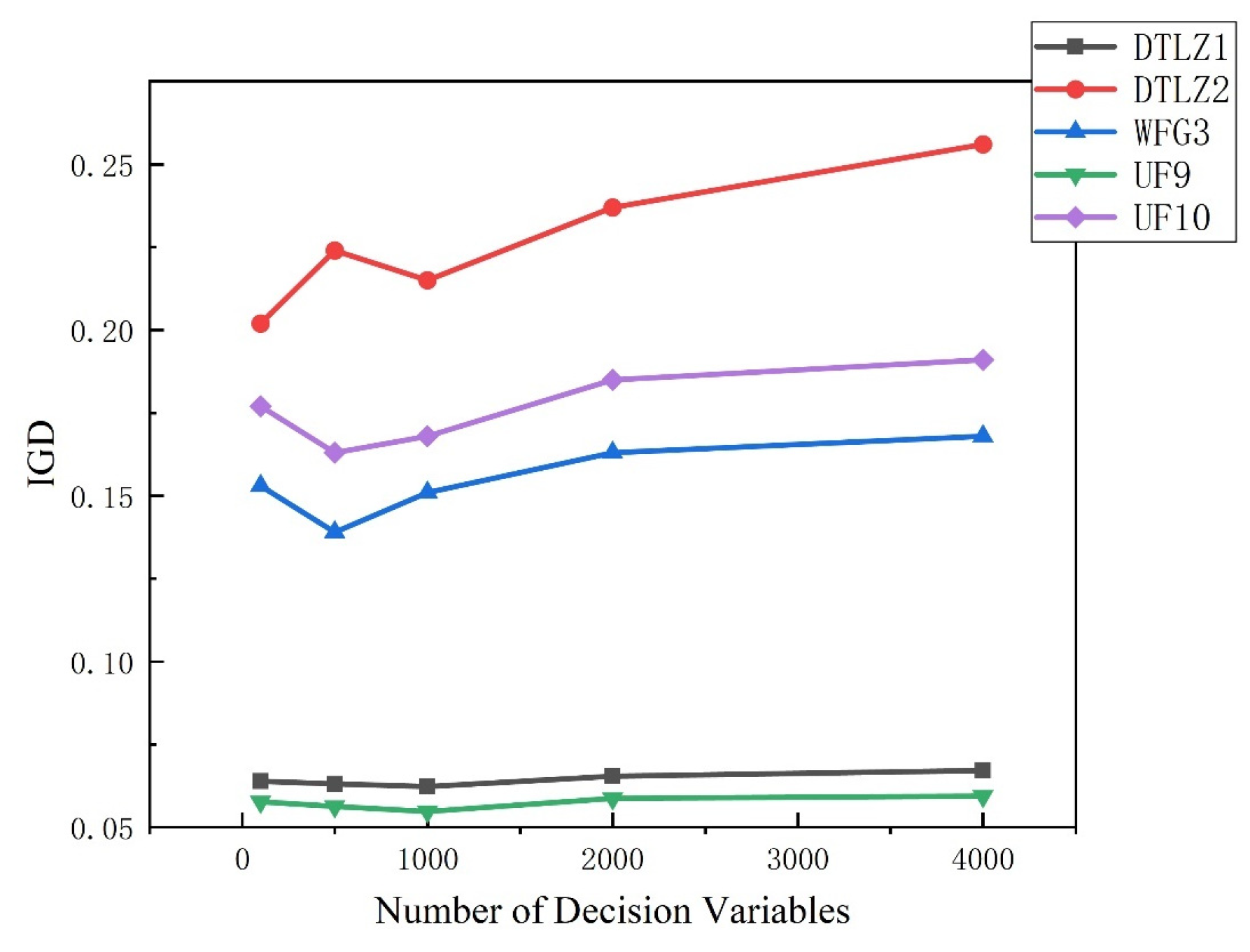
4.2.3. Performance of LMEA on Large-Scale MaOPs with 2000 and 4000 Decision Variables

In the previous part, we proved the excellent performance of the proposed algorithm LSMOEA-VT when the number of decision variables is from 100 to 1000. In this part, we further studied the performance of LSMOEA-VT when there are more decision variables.

Table 3. HV metric values of LMEA on DTLZ1–DTLZ7, WFG3, UF9, and UF10, with 2000 and 4000 decision variables.

Problem	Obj.	2000-Variable	4000-Variable
DTLZ1	5	9.3525 × 10−1 (7.37 × 10−3)	9.3571 × 10−1 (5.36 × 10−3)
DTLZ2	5	6.2454 × 10−1 (5.17 × 10−3)	6.2331 × 10−1 (4.65 × 10−3)
DTLZ3	5	6.2466 × 10−1 (4.94 × 10−3)	6.2370 × 10−1 (1.53 × 10−2)
DTLZ4	5	5.7154 × 10−1 (4.53 × 10−2)	5.8147 × 10−1 (2.34 × 10−2)
DTLZ5	5	3.3281 × 10−2 (2.87 × 10−4)	3.2918 × 10−2 (3.49 × 10−4)
DTLZ6	5	3.3110 × 10−2 (1.41 × 10−3)	3.4250 × 10−2 (1.37 × 10−4)
DTLZ7	5	1.2547 × 10−1 (4.85 × 10−3)	1.2963 × 10−1 (3.10 × 10−3)
WFG3	5	5.8532 × 10−1 (2.54 × 10−3)	5.8791 × 10−1 (3.76 × 10−3)
UF9	3	7.0363 × 10−1 (1.49 × 10−2)	7.1057 × 10−1 (1.22 × 10−2)
UF10	3	1.6887 × 10−1 (7.96 × 10−3)	1.6449 × 10−1 (1.60 × 10−2)

shows the performance of the proposed LSMOEA-VT algorithm on DTLZ1, DTLZ7, WFG3, UF9, and UF10 when the decision variables are 2000 and 4000, respectively. From the table, we can see that LSMOEA-VT has obtained similar HV indicators on each test problem.

For further observation, Figure 4 shows the IGD index values of LSMOEA-VT on DTLZ 1, DTLZ 2, WFG3, UF9, and UF10, and 20 independent operation comparisons are made when the number of decision variables is 100, 500, 1000, 2000, and 4000. From the figure, we can see that with the increase of the number of decision variables, the IGD index obtained by LSMOEA-VT on test problems has hardly decreased, which shows that the LSMOEA-VT algorithm proposed by us has good scalability.

4.2.4. Efficiency Comparison Between LSMOEA-VT and Other Algorithms

In order to further study the performance of LSMOEA-VT, we compare the running time of five algorithms on some test problems, in which the number of decision variables of DTLZ1, DTLZ2, WFG3, UF9, and UF10 is 100, and the number of LSMOEA-VT is 300. The results are shown in

Table 4. Average runtimes (s) of five algorithms on some test problems.

Problem	NSGA-III	MOEA/D	MOEA/DVA	LMEA	LSMOEA-VT
DTLZ1	5.4198 × 10+1	4.5699 × 10+2	2.8743 × 10+2	5.9040 × 10+1	5.3691 × 10+1
DTLZ2	6.6541 × 10+1	6.0568 × 10+2	3.5147 × 10+2	5.5374 × 10+1	5.1817 × 10+1
WFG3	6.6261 × 10+1	6.4752 × 10+2	3.5863 × 10+2	5.2783 × 10+1	5.0770 × 10+1
UF9	6.9655 × 10+1	6.3372 × 10+2	3.5215 × 10+2	5.5708 × 10+1	4.9766 × 10+1
UF10	6.7915 × 10+1	6.3627 × 10+2	3.6118 × 10+2	6.2106 × 10+1	5.2047 × 10+1
LSMOP1	7.9914 × 10+1	8.2347 × 10+2	2.5079 × 10+2	1.60002× 10+2	3.4328 × 10+2
LSMOP2	8.6011 × 10+1	8.1857 × 10+2	2.4873 × 10+2	1.4634 × 10+2	3.4029 × 10+2
LSMOP3	8.9809 × 10+1	8.3215 × 10+2	2.7383 × 10+2	1.3938 × 10+2	3.4699 × 10+2

. From the table, we can see that LSMOEA-VT spends the least time on DTLZ1, DTLZ 2, WFG3, UF9, and UF10 issues, and the time spent on the LMEA algorithm based on the grouping strategy is also much less than MOEA/DVA, because MOEA/DVA spends a lot of time on the analysis of decision variables, resulting in poor performance. At the same time, on the LSMOP test suite, because the program is relatively simple and ignores the impact of performance, NSGA-III takes the least time among all algorithms. The time required for LSMOEA-VT is longer than that for LMEA. This is because the computational cost for maintaining the population diversity in the LSMOEA-VT algorithm is higher than that of LMEA. Therefore, although the population diversity in the LSMOEA-VT algorithm is increased, it consumes more computational resources.

5. Conclusions and Future Work

In this paper, a two-stage large-scale optimization algorithm based on decision variable clustering (LSMOEA-VT) is proposed to solve large-scale optimization problems. The decision variables are classified in LSMOEA-VT, and the dimension reduction method is used to optimize the variables that affect the evolutionary convergence. Then, a non-dominated dynamic weight aggregation method is used to solve a set of single-objective optimization problems with reference lines through Pareto optimal subspace to enhance the diversity of the population. In the above experiments, we have carried out experimental comparisons on some low-dimensional benchmark functions, namely the UF test suite, and the experiments show that we can obtain satisfactory results with less computational cost. In addition, we also compared with other algorithms on DTLZ, WFG, and UF test suites when the decision variable is 100, 500, and 1000, and obtained satisfactory results in convergence and diversity, thus verifying the effectiveness and efficiency of our algorithm. Finally, we also try the problem of 4000 decision variables to verify the scalability of our algorithm.

Although our algorithm has excellent performance in solving large-scale optimization problems, there are still some problems to be solved. First, in the first stage of decision variables, we simply divide the decision variables into convergence correlation and diversity correlation; even the grouped decision variables may have different correlations with the objective function, and whether there is a more accurate classification method. It consumes a lot of computing resources in the decision variable grouping stage. Therefore, how to deal with these variables efficiently is a very valuable research problem. In addition, in real society, due to the complexity of decision variables, how to use our algorithm to solve these practical application problems may be an interesting direction.

References

1. Deb, K.; Pratap, A.; Agarwal, S.; Meyarivan, T. A fast and elitist multiobjective genetic algorithm: NSGA-II. IEEE Trans. Evol. Comput. 2002, 6, 182–197. [Google Scholar] [CrossRef]
2. Zhang, Q.; Li, H. MOEA/D: A multiobjective evolutionary algorithm based on decomposition. IEEE Trans. Evol. Comput. 2007, 11, 712–731. [Google Scholar] [CrossRef]
3. Deb, K.; Jain, H. An evolutionary many-objective optimization algorithm using reference-point-based nondominated sorting approach, part i: Solving problems with box constraints. IEEE Trans. Evol. Comput. 2014, 18, 577–601. [Google Scholar] [CrossRef]
4. Liu, C.; Liu, J.; Jiang, Z. A multiobjective evolutionary algorithm based on similarity for community detection from signed social networks. IEEE Trans. Cybern. 2014, 44, 2274–2287. [Google Scholar]
5. Zhu, H.; Shi, Y. Brain storm optimization algorithm for full area coverage of wireless sensor networks. In Proceedings of the 2016 Eighth International Conference on Advanced Computational Intelligence (ICACI), Chiang Mai, Thailand, 14–16 February 2016; pp. 14–20. [Google Scholar]
6. Guo, Y.; Liu, D.; Chen, M.; Liu, Y. An energy-efficient coverage optimization method for the wireless sensor networks based on multi-objective quantum-inspired cultural algorithm. In Proceedings of the Advances in Neural Networks ISNN 2013, Dalian, China, 4–6 July 2013; pp. 343–349. [Google Scholar]
7. Fleming, P.J.; Purshouse, R.C.; Lygoe, R.J. Many-objective optimization: An engineering design perspective. In Proceedings of the 3rd International Conference on Evolutionary Multi-Criterion Optimization, Guanajuato, Mexico, 9–11 March 2005; pp. 14–32. [Google Scholar]
8. Garcia, J.; Berlanga, A.; López, J.M.M. Effective evolutionary algorithms for many-specifications attainment: Application to air traffic control tracking filters. IEEE Trans. Evol. Comput. 2009, 13, 151–168. [Google Scholar]
9. Kollat, J.B.; Reed, P.M.; Maxwell, R.M. Many-objective groundwater monitoring network design using bias-aware ensemble Kalman filtering, evolutionary optimization, and visual analytics. Water Resour. Res. 2011, 47, 1–18. [Google Scholar] [CrossRef]
10. Potter, M.A.; Jong, K.A.D. A cooperative coevolutionary approach to function optimization. Third Parallel Prob. Solving Form Nat. 1994, 866, 249–257. [Google Scholar]
11. Li, X.; Mei, Y.; Yao, X.; Omidvar, M.N. Cooperative co-evolution with differential grouping for large scale optimization. IEEE Trans. Evol. Comput. 2014, 18, 378–393. [Google Scholar]
12. Chen, W.; Weise, T.; Yang, Z.; Tang, K. Large-scale global optimization using cooperative coevolution with variable interaction learning. In Proceedings of the International Conference on Parallel Problem Solving from Nature, Krakow, Poland, 11–15 September 2010; pp. 300–309. [Google Scholar]
13. Sun, Y.; Kirley, M.; Halgamuge, S.K. Extended differential grouping for large scale global optimization with direct and indirect variable interactions. In Proceedings of the 2015 Annual Conference on Genetic and Evolutionary Computation, Madrid, Spain, 11–15 July 2015; pp. 313–320. [Google Scholar]
14. Omidvar, M.N.; Li, X.; Yao, X. Cooperative co-evolution with delta grouping for large scale non-separable function optimization. In Proceedings of the IEEE Congress on Evolutionary Computation, New Orleans, LA, USA, 5–8 June 2011; pp. 1–8. [Google Scholar]
15. Yang, Z.; Tang, K.; Yao, X. Multilevel cooperative coevolution for large scale optimization. In Proceedings of the IEEE Congress on Evolutionary Computation, Hong Kong, China, 1–6 June 2008; pp. 1663–1670. [Google Scholar]
16. Zhang, X.; Tian, Y.; Cheng, R.; Jin, Y. A decision variable clustering-based evolutionary algorithm for large-scale many-objective optimization. IEEE Trans. Evol. Comput. 2016, 22, 97–112. [Google Scholar] [CrossRef]
17. Hajikolaei, K.H.; Pirmoradi, Z.; Cheng, G.H.; Wang, G.G. Decomposition for large-scale global optimization based on quantified variable correlations uncovered by metamodeling. Eng. Optim. 2015, 47, 429–452. [Google Scholar] [CrossRef]
18. Ghorpadeaher, J.; Metre, V.A. Clustering multidimensional data with PSO based algorithm. arXiv 2014, arXiv:1402.6428. [Google Scholar]
19. Chen, W.N.; Zhang, J.; Chung, H.S.H.; Zhong, W.L.; Wu, W.G.; Shi, Y.H. A novel set-based particle swarm optimization method for discrete optimization problems. IEEE Trans. Evol. Comput. 2010, 14, 278–300. [Google Scholar] [CrossRef]
20. Chen, W.N.; Zhang, J.; Lin, Y.; Chen, N.; Zhan, Z.H.; Chung, S.H.; Li, Y.; Shi, Y.H. Particle swarm optimization with an aging leader and challengers. IEEE Trans. Evol. Comput. 2013, 17, 241–258. [Google Scholar] [CrossRef]
21. Yu, W.J.; Shen, M.; Chen, W.N.; Zhan, Z.H.; Gong, Y.J.; Lin, Y.; Liu, O.; Zhang, J. Differential evolution with two-level parameter adaptation. IEEE Trans. Cybern. 2014, 44, 1080–1099. [Google Scholar] [CrossRef]
22. Ma, X.; Liu, F.; Qi, Y.; Wang, X.; Li, L.; Jiao, L. A multiobjective evolutionary algorithm based on decision variable analyses for multiobjective optimization problems with large-scale variables. IEEE Trans. Evol. Comput. 2015, 20, 275–298. [Google Scholar] [CrossRef]
23. Wolfe, D.A.; Hollander, M. Nonparametric statistical methods. In Biostatistics and Microbiology: A Survival Manual; Springer: New York, NY, USA, 2009. [Google Scholar]
24. Zille, H.; Ishibuchi, H.; Mostaghim, S.; Nojima, Y. A framework for large-scale multiobjective optimization based on problem transformation. IEEE Trans. Evol. Comput. 2018, 22, 260–275. [Google Scholar] [CrossRef]
25. He, C.; Li, L.; Tian, Y.; Zhang, X.; Cheng, R.; Jin, Y.; Yao, X. Accelerating Large-Scale Multiobjective Optimization via Problem Reformulation. IEEE Trans. Evol. Comput. 2019, 23, 949–961. [Google Scholar] [CrossRef]
26. Zhang, X.; Zheng, X.; Cheng, R.; Qiu, J.; Jin, Y. A competitive mechanism based multi-objective particle swarm optimizer with fast convergence. Inf. Sci. 2018, 427, 63–76. [Google Scholar] [CrossRef]
27. Cheng, R.; Jin, Y. A competitive swarm optimizer for large scale optimization. IEEE Trans. Cybern. 2015, 45, 191–204. [Google Scholar] [CrossRef]
28. Zhang, Y.; Wang, G.-G.; Li, K.; Yeh, W.-C.; Jian, M.; Dong, J. Enhancing MOEA/D with information feedback models for large-scale many-objective optimization. Inf. Sci. 2020, 522, 1–16. [Google Scholar] [CrossRef]
29. Cheng, R.; Jin, Y.; Narukawa, K.; Sendhoff, B. A multiobjective evolutionary algorithm using gaussian process-based inverse modeling. IEEE Trans. Evol. Comput. 2015, 19, 838–856. [Google Scholar] [CrossRef]
30. Deb, K.; Thiele, L.; Laumanns, M.; Zitzler, E. Scalable Test Problems for Evolutionary Multiobjective Optimization; Springer: London, UK, 2005. [Google Scholar]
31. Huband, S.; Hingston, P.; Barone, L.; While, L. A review of multiobjective test problems and a scalable test problem toolkit. IEEE Trans. Evol. Comput. 2006, 10, 477–506. [Google Scholar] [CrossRef]
32. Zhang, Q.; Zhou, A.; Zhao, S.; Suganthan, P.N.; Liu, W.; Tiwari, S. Multiobjective Optimization Test Instances for the CEC 2009 Special Session and Competition; Nanyang Technological University: Singapore, 2008; Volume 264, pp. 1–30. [Google Scholar]
33. Cheng, R.; Jin, Y.; Olhofer, M.; Sendhoff, B. Test problems for largescale multi- and many-objective optimization. IEEE Trans. Cybern. 2017, 47, 4108–4121. [Google Scholar] [CrossRef] [PubMed]
34. Zhou, A.; Jin, Y.; Zhang, Q.; Sendhoff, B.; Tsang, E. Combining model-based and genetics-based offspring generation for multi-objective optimization using a convergence criterion. In Proceedings of the IEEE International Conference on Evolutionary Computation, Vancouver, BC, Canada, 16–21 July 2006; pp. 892–899. [Google Scholar]
35. While, L.; Hingston, P.; Barone, L.; Huband, S. A faster algorithm for calculating hypervolume. IEEE Trans. Evol. Comput. 2006, 10, 29–38. [Google Scholar] [CrossRef]
Figure 1. Examples of the loss of population diversity in the LSMOEA solution. (a) Early evolution; (b) Metaphase of evolution; (c) End of evolution.
Algorithms 18 00164 g001
Figure 2. The PF obtained by five algorithms on UF2 function with 30 decision variables. (a) NSGA-III; (b) MOEA/D; (c) MOEA/DVA; (d) LMEA; (e) LSMOEA-VT.
Algorithms 18 00164 g002
Figure 3. The PF obtained by five algorithms on UF4 function with 30 decision variables. (a) NSGA-III; (b) MOEA/D; (c) MOEA/DVA; (d) LMEA; (e) LSMOEA-VT.
Algorithms 18 00164 g003
Figure 4. IGD metric values of LSMOEA-VT on DTLZ1, DTLZ2, WFG3, UF9, and UF10 with different numbers of decision variables.
Algorithms 18 00164 g004