Prediction of Diabetes Using Statistical and Machine Learning Modelling Techniques

Abstract

Statistical and machine learning modelling techniques have been effectively used in the healthcare domain and the prediction of epidemiological chronic diseases such as diabetes, which is classified as an epidemic due to its high rates of global prevalence. These techniques are useful for the processes of description, prediction, and evaluation of various diseases, including diabetes. This paper models diabetes disease in Saudi Arabia using the most relevant risk factors, namely smoking, obesity, and physical inactivity for adults aged ≥25 years. The aim of this study is based on developing statistical and machine learning models for the purpose of studying the trends in incidence rates of diabetes over 15 years (1999–2013) and to obtain predictions for future levels of the disease up to 2025, to support health policy planning and resource allocation for controlling diabetes. Different models were developed, namely Multiple Linear Regression (MLR), Support Vector Regression (SVR), Bayesian Linear Regression (BLM), Adaptive Neuro-Fuzzy Inference model (ANFIS), and Artificial Neural Network (ANN). The performance of the developed models is evaluated using four statistical metrices: Mean Squared Error (MSE), Root Mean Squared Error (RMSE), Mean Absolute Percentage Error (MAPE), and coefficient of determination R-squared. Based on the results, it can be observed that the overall performance for all proposed models was reasonably good; however, the best results were achieved by the ANFIS model with RMSE = 0.04 and R² = 0.99 for men’s training data, and RMSE = 0.02 and R² = 0.99 for women’s training data.

1. Introduction

Diabetes is a serious health problem that is growing significantly around the world because of several demographic and behavioural factors, including increasing population density, urbanisation, an aging population, the prevalence of obesity, and low physical activity. Diabetes Mellitus (DM) is a group of metabolic disorders characterised by chronic hyperglycaemia due to deficiencies in insulin production, resistance to insulin, or both. This condition leads to abnormalities in the metabolism of carbohydrates, fats, and proteins, and, over time, it can result in complications affecting various organs, including the eyes, kidneys, nerves, heart, and blood vessels [1,2]. There are three types of diabetes classified according to aetiology and clinical picture: type 1 diabetes, type 2 diabetes, and gestational diabetes. Patients with type 1 diabetes need insulin injections to survive, while type 2 diabetes, which represents most cases, is a defect in the secretion and function of insulin, meaning some diabetics of this type need insulin but most do not as they continue to produce insulin. Gestational diabetes is recognised or first starts during pregnancy, which is characterised by glucose intolerance of varying degrees of severity [3].

Chronic diseases such as diabetes that are associated with lifestyle factors have become the most prevalent and the most significant threat to health. The increasing rate of diabetes and its associated complications has been reaching an alarming level worldwide. The prevalence rate of diabetes is higher in developed countries than in developing countries; however, during the past two decades, diabetes has been reported at higher levels in developing countries [4]. Official statistics published by the International Diabetes Federation (IDF) indicate that there were more than 460 million people with diabetes in 2019; this figure is expected to increase to 578 million in 2030, and 700 million in 2045. The IDF also reported that in the Kingdom of Saudi Arabia (KSA), the case of our study, there are currently an estimated 4 million diabetic patients [5].

The increasing prevalence of diabetes has prompted researchers around the world to investigate methods for the prediction and early diagnosis of diabetes. A variety of published studies have predicted the incidence of diabetes and its global prevalence for different countries around the world, including the KSA, using diverse data and methods of analysis. Future estimates of the burden of diabetes are very important for health policy planning and resource allocation [6,7]. Recently, machine learning algorithms have been widely used in public health for predicting or diagnosing epidemiological chronic diseases, including DM. There are many published diabetes studies that used different machine learning techniques, including Support Vector Machines (SVMs), Artificial Neural Network (ANN), K-Nearest Neighbour (KNN), fuzzy logic (FL), and decision tree [8,9].

This study contributes to developing different statistical and machine learning methods, namely Multiple Linear Regression (MLR), Adaptive Neuro-Fuzzy Interference System (ANFIS), Artificial Neural Network (ANN), Support Vector Regression (SVR) and Bayesian Linear Regression (BLR), for the purpose of describing the prevalence pattern of diabetes and obtaining predictions of the future level of the disease. The rest of the paper is organised as follows: Section 2 reviews the literature. Section 3 presents the proposed methodologies. Section 4 introduces the experimental methodology. Section 5 presents the results. Section 6 provides a discussion of the findings. Finally, Section 7 concludes this paper and identifies areas for future research.

2. Literature Review

In the last few decades, several studies have predicted the incidence of diabetes and its global prevalence for different countries around the world, using diverse data and methods of analysis. King et al. [10] estimated diabetes prevalence by the number of diabetics aged 20 years and over for every country in the world in three time points: 1995, 2000, and 2025. Other variables were calculated, such as the gender proportion, urban–rural proportion, and age groups of the population who suffer diabetes. The data used in this study were obtained from the World Health Organisation’s (WHO) global database, which was collected from 75 societies representing 32 countries. To estimate the number of diabetes cases in every country in the world, data gathered from the WHO were linked to demographic estimates and projections released by the United Nations. The study assumed that, besides ethnicity, other factors contribute to diabetes trends, such as population size, sex, age structure, and urbanisation level. All data sources were analysed using logistic regression modelling. The global prevalence of diabetes in 1995 was estimated to be 4.0%, predicted to increase to 5.4% by the year 2025. This was higher in developed than developing countries. Wild et al. [11] developed an updated report in 2004, adding new data and various techniques to estimate age-specific diabetes prevalence. This study estimated the prevalence of diabetes, and the number of diabetics in all age groups, for the years 2000 and 2030. For this study, diabetes prevalence data according to age and sex were collected from a restricted range of countries and extrapolated to all 191 states represented by the WHO. For people aged 20 and over, the data were obtained using population-based studies, using WHO criteria for diagnosing diabetes. In order to generate smooth, age-specific estimates, DisMod II version 1.01 software was used, which is a mathematical model for analysing estimations of disease with regard to occurrences, prevalence, and mortality rates. It was estimated that the global prevalence of diabetes for all age groups was 2.8% in 2000, projected to rise to 4.4% in 2030; a total of 171 million diabetic people in 2000 was predicted to increase to 366 million by 2030. A study by Shaw et al. [12] aimed to predict the number of diabetes cases globally for 2010 and 2030. Studies were collected from the 91 countries in which they were published between January 1989 and March 2009. A total of 133 studies that used a population-based method to evaluate the prevalence of diabetes were selected, applying the diagnostic measures of the WHO or the American Diabetes Association (ADA). Age- and sex-specific diabetes prevalence in people aged 20–79 was calculated using logistic regression modelling. These calculations were applied to the estimates of national populations to estimate the number of diabetic people for all 216 countries for 2010 and 2030. It was estimated that the global prevalence of diabetes within the 20–79 age group was 285 million adults in 2010, projected to rise to 439 million by 2030.

The recent literature has produced a significant amount of research on diabetes using several techniques. These techniques have been used for various purposes, such as diagnosing or detecting diabetes at an early stage, and for modelling the disease’s progression and complications. A study by Mukasheva et al. [13] used three different types of regression analysis methods, linear, polynomials, and exponential, to develop models for predicting the number of diabetic patients in Kazakhstan in 2019. Their study aimed to develop a model that can predict the increase in the number of diabetics using regression analysis methods, and to identify the most effective experimental method for predicting diabetes. The data of diabetic patients were obtained from a public foundation, the Kazakh Society for the Study of Diabetes. Data on patients with diabetes from 2004 to 2018 were used to build predictive models by finding patterns over the last 15 years, and then these models could accurately predict the prevalence of diabetes in Kazakhstan. The proposed models were implemented in scikit-learn library for the Python programming language and Microsoft Excel software. The results showed that the number of diabetes patients will increase, and that there was a strong correlation of population growth with the increase in the number of diabetic patients. Their findings indicated that all the three types of regression had high coefficients of determination R² which was always above 0.90; however, the polynomial regression model achieved the highest R² value, which means it was the best suited for predicting the number of diabetes patients. Another study performed by Islam et al. [14] developed the random forest (RF) and extreme gradient boosting (XGB) regression models and an ensemble model based on linear combination of the RF and XGB models for HbA1c prediction. These models were used to predict the average amount of glucose accumulated in the blood over the last 2–3 months using past continuous glucose monitoring (CGM) data. Predicting the levels of HbA1c in advance helps to determine direct relationships with diabetes and to avoid the future risk of complications. In this study, the dataset was collected from the Diabetes Research in Children Network (DirecNet) trials on a total of 170 patients having T1DM. Furthermore, various methods for feature extraction and selection were used to prepare the dataset. The findings obtained by this study show that the best performance was achieved by the constructed model which involved two ensemble methods, RF and extreme gradient boosting (XGB), with a low mean absolute error (MAE) of 3.39 mmol/mol and a high score of coefficients of determination R² of 0.81.

Patil et al. [15] aimed to evaluate the performance of classification algorithms on the prediction of diabetes. In this study, the PIMA Indian data repository was used, which included a total of 768 samples. These data were divided into training and testing sets, with 70% for training (538 samples) and 30% for testing (230 samples). This study examined the implementation of eight machine learning models, namely logistic regression (LR), (KNN), (SVM), Gradient Boost, decision tree, Multilayer Perceptron (MLP), random forest, and Gaussian Naïve Bayes. The results showed that the highest accuracy was achieved by the logistic regression model, with 79.54% and RMSE of 0.4652; the lowest accuracy was given by the Multilayer Perceptron (MLP), with 64.07% and RMSE of 0.5994. The authors suggested improving the obtained results by using outlier detection before classification. A comparative study conducted by Faruque et al. [16] used different machine learning models, including SVM, C4.5 decision tree, Naïve Bayes, and KNN, and used the evaluation metrics of accuracy, recall, and precision to compare the performance of the classification models on predicting diabetes. In their study, they collected diabetes data from the diagnostics of Medical Centre Chittagong (MCC), Bangladesh. The dataset includes 200 patients with various attributes such as age, sex, weight, blood pressure, and other risk factors. The results obtained from this study indicated that the best performance was achieved by the C4.5 decision tree model with an accuracy of 73%. In another study, Oleiwi et al. [17] proposed a classification model aimed at the early detection of diabetes using machine learning algorithms. This study was designed to use significant features and deliver results which are close to the clinical outcomes. The data used in this study were collected from patients using direct questionnaires from the Diabetes Hospital of Sylhet, Bangladesh. This dataset includes reports of diabetes-related symptoms of 520 instances with 16 attributes. The authors used two class variables to find whether the patient had a risk of diabetes (positive) or not (negative). Three classification models were trained, namely Multilayer Perceptron (MLP), radial basis function network (RBF), and random forest (RF), mainly to obtain the best classifier model for predicting diabetes. Their findings showed that the RBF model outperformed other models, with an accuracy of 98.80%. Abdulhadi et al. [18] developed a variety of machine learning models for the purpose of predicting the presence of diabetes in females using the PIDD dataset. They addressed the problem of missing values using the mean substitution technique, and all attributes were rescaled using a standardisation method. The constructed models are linear discriminant analysis (LDA), LR, SVM (linear and polynomial), and random forest (RF). Based on the results of their study, the highest accuracy score was achieved by the RF model, with 82%.

Further to the studies that predicted or diagnosed diabetes, some existing studies have addressed the use of machine learning techniques to construct predictive models for diabetes complications. Dagliati et al. [19] developed different classification models including LR, NB, SVMs, and random forest to predict the onset of retinopathy, neuropathy, and nephropathy in T2DM patients. The authors used different time scenarios for making predictions, namely 3, 5, and 7 years from the first visit to the hospital for diabetes treatment. The dataset used to train the proposed models was collected by Istituto Clinico Scientifico Maugeri (ICSM), Hospital of Pavia, Italy, for longer than 10 years. These data involve a total number of 943 records including the features of gender, age, BMI, time from diagnosis, hypertension, glycated haemoglobin (HbA1c), and smoking habit. The problem of unbalanced and missing data was managed by applying the miss forest approach, while the problem of unbalanced class was overcome by oversampling the minority class. The obtained results of this study show that the highest accuracy score was achieved by LR with 77.7%.

Another example is the model developed by Kantawong et al. [20] to predict some complications related to diabetes, particularly hyperlipidaemia, coronary heart disease, kidney disease, and eye disease. A dataset of 455 records was used in this study. Selection and cleaning process were carried out on the dataset which reduced the number of records used to build the model. The number of features and the final number of records which were used to train the model were not mentioned by the authors. An iterative decision tree (ID3) algorithm was chosen to construct the model. For evaluating the performance of the proposed model, a 10-fold cross validation method was used, giving an accuracy of 92.35%. It should be noted that the high accuracy score obtained by this study is not sufficient to evaluate the performance of the model, especially when training unbalanced data. The main reason for this is that when the model trains the data, a minority class can be ignored, and all the predictions are classified as the majority class and the good accuracy scores are still achieved.

Although machine learning methods have been utilised in other aspects of diabetes research, most of them are based on diagnosing or detecting the disease, and little research attention has explored the adoption of machine learning methods to study the trends in the prevalence of diabetes and forecast its future in specific populations such as in the KSA. Thus, this paper attempts to apply various machine learning methods for studying diabetes prevalence rates and the predicted trends of the disease according to the related behavioural risk factors in the KSA.

3. Methodologies

3.1. Models Overview

This section provides a brief overview of the models used for diabetes prediction, including Multiple Linear Regression (MLR), Bayesian Linear Regression (BLR), Support Vector Regression (SVR), Artificial Neural Network (ANN), and the Adaptive Neuro-Fuzzy Inference System (ANFIS). It highlights the mathematical foundations of these models and their unique operational characteristics.

These models were selected based on their ability to handle regression tasks with varying levels of complexity. MLR and BLR serve as interpretable benchmarks, offering a foundation for comparison. SVR was chosen for its ability to mitigate overfitting through margin optimisation, while ANN effectively captures complex nonlinear relationships. ANFIS was selected for its hybrid nature, combining rule-based inference with neural adaptability. This diverse selection ensures a balanced evaluation of accuracy, interpretability, and computational efficiency, facilitating a comprehensive comparison between traditional regression techniques and advanced machine learning approaches to identify the most effective model.

• Multiple Linear Regression

Multiple Linear Regression is one of the most common types of linear regression analysis. It is an extended form of simple linear regression, with a relationship between more than two variables [21]. In predictive analysis, this technique describes the relationship between one dependent (response) variable and two or more independent (predictor) variables. The general model of Multiple Linear Regression is

$$Y={\beta }_0+{\beta }_1{X}_1+{\beta }_2{X}_2+\dots +{\beta }_n{X}_n$$

(1)

where $Y$ is the dependent variable; ${\beta }_0,{\beta }_1,{\beta }_2,{\dots ,\beta }_n$ are the coefficients; and $X_1,X_2,\dots ,X_n$ are the independent variables.

2.

Bayesian Linear Regression

Bayesian Linear Regression is based on a generative method, which is different from a discriminant one which depends on Bayesian inference to build linear regression models [22]. Once the model is specified, the posterior distribution of parameters and forecasts of the model are computed by the method. This statistical analysis enables the method to define the complexity of the model through training, which produces a model with few possibilities to overfit. In contrast to the simple linear regression model, the responses in Bayesian Linear Regression are assumed as samples from the probability distribution, for example the normal (Gaussian) distribution, which is

$$Y~N\left({\beta }^{T}X,{\sigma }^2\right)$$

(2)

The product of the parameters β and the inputs X is the mean of the Gaussian, where the normal deviation is σ. As well as the responses, in Bayesian models the parameters are also supposed to be sampled from a distribution. The aim is to define the posterior probability distribution for the parameters of the model with given X inputs and Y outputs, as in Equation (3):

$$P\left(\beta |Y,X\right)={\displaystyle \frac{P\left(Y | \beta ,X\right)P\left(\beta |X\right)}{P\left(Y|X\right)}}$$

(3)

The result obtained from modelling by Bayesian Linear Regression is not a single estimate, but rather a distribution range which can be used to produce inferences regarding new observations. This distribution enables the determination of uncertainty in the model, which is considered one of the advantages of Bayesian modelling methods. When the volume of data increases, the uncertainty of the result declines, presenting a better level of certainty in the approximation [23].

3.

Support Vector Regression

Support Vector Machine (SVM) is a popular method developed by Vapnik. The generalised concepts of SVM have been applied to regression problems such as modelling and prediction and accordingly called Support Vector Regression (SVR). SVR has been effectively utilised to deal with forecasting issues in many areas as diverse as pharmacology, economics, and power systems analysis. SVR is less popular than SVM, but it has been verified that it is a valuable technique in estimating the real value of a function [24]. One of the most useful features of SVM is that the complexity of its computation does not rely on the dimensional parameters of the input space. Moreover, SVR shows better generalisation ability, with high performance and accurate prediction. Fundamentally, SVR is a linear approach with one output, dealing with a high-dimensional feature space established by nonlinear mapping of the N-dimensional input vector into a K-dimensional feature space (K > N) utilising the function $\phi$(x). The learning process is moved to the minimisation of the error function, which is defined by the so called ε-insensitive loss function $L_{\epsilon }\left(d,y\left(x\right)\right)$:

$$L_{\epsilon }\left(d,y\left(x\right)\right)=\left\{\begin{array}{c}\left|d-y\left(x\right)\right|-\epsilon , for \left|d-y\left(x\right)\right|\ge \epsilon \\ 0, for \left|d-y\left(x\right)\right|<\epsilon \end{array}\right.$$

(4)

where ε is the assumed accuracy; d is the destination; x is the input vector; and y(x) is the actual output under the effect of x. The actual output of the SVR is defined by

$$y\left(x\right)={\sum }_{j=1}^K{\omega }_j{\phi }_j\left(x\right)+b=w^T\phi \left(x\right)+b$$

(5)

where $w=[{\omega }_0,{\omega }_1,\dots ,{\omega }_K{]}^T$ is the weight vector; and $\phi \left(x\right)=\left[{\phi }_0\right(x),{\phi }_1(x),\dots ,{\phi }_K{\left(x\right)]}^T$ is the basis function vector.

4.

Adaptive Neuro-Fuzzy Inference Model

The ANFIS model is a combined model of fuzzy systems and ANN [25]. The main parts of the FIS are fundamental rules, which contain the choices of fuzzy logic rules “If-Then”, a set of membership functions, and the fuzzy logic inference procedures from the fundamental rules to obtain the output. In order to map the inputs with the outputs, two common fuzzy inference systems (FIS) can be employed in different applications: Mamdani and Sugeno inference systems.

The fuzzy rules in the two inference models give different results, therefore their actions of defuzzification and combination are also different. However, the Sugeno system is believed to be computationally more efficient than the Mamdani; in the former, the resultant parameter is a linear equation or constant coefficient. Supposing that we have a system including two inputs, x and y, and the output is f, and the based rule has two fuzzy if-then rules, then the description of rules for the linear equation Sugeno FIS can be presented as rule 1 (R1) and rule 2 (R2):

$$\mathrm{R}\mathrm{1:} \mathrm{if} x \mathrm{i}\mathrm{s} A_1\mathrm{and} y \mathrm{i}\mathrm{s} B_1\mathrm{then} f_1=p_{1}x+q_{1}y+r_1$$

(6)

$$\mathrm{R}\mathrm{2:} \mathrm{if} x \mathrm{i}\mathrm{s} A_2\mathrm{and} y \mathrm{i}\mathrm{s} B_2\mathrm{then} f_2=p_{2}x+q_{2}y+r_2$$

(7)

where $A_i$ and $B_i$ are the membership functions of each input $x$ and $y$; and $p_i{,q}_i$ and $r_i$ are the linear parameters in the resulting part of the Sugeno fuzzy inference system.

The ANFIS model can be considered successful due to the strength of its results. Moreover, as with other machine learning techniques and as a neural network, ANFIS has a high ability to generalise. On the other hand, there are some limitations of the ANFIS model regarding the type, number, and position of membership functions [26].

5.

Artificial Neural Networks Model

Neural Network and ANN are mathematical models based on the concept of Artificial Intelligence, which simulates the biological neuronal activity of the human brain. This modelling approach is a valuable tool that simulates the functionality of the human brain when dealing with complex relations between the inputs and outputs in any system [27]. There are many types of ANN architectures, the most common of which is Multilayer Perceptron (MLP), which is commonly used for prediction. It comprises three layers: an input layer, hidden layers, and an output layer. Supposing that the input vector is $\overrightarrow{x}$ and the weight vector is $\overrightarrow{w}$, and the activation function is a sigmoid function (which is the most commonly used function type), the output is given by

$$Y=sigmoid\left({\overrightarrow{w}}^T.\overrightarrow{x}\right)$$

(8)

where the sigmoid(x) is

$$sigmoid\left(x\right)={\displaystyle \frac{1}{1+e^{-x}}}$$

(9)

One of the characteristic advantages of the Neural Network technique is its ability to deal with noisy, incomplete, or missing data, requiring no previous assumptions. In addition, it has capabilities to deal with complex relations between input and output variables, and consequently to predict the output of new data input. However, overfitting and overtraining are considered as limitations of Neural Networks. Additionally, regarding the selection of parameters, in Neural Network there is no formal way to select the suitable parameters for the model, which may influence the accuracy of its prediction.

3.2. Performance Evaluation Measures

• Mean Squared Error

MSE is the most popular and simple interpreted metric for many types of regression models. It measures how close a regression line is to a set of data points. This can be calculated by taking the distances (errors) from the points to the regression line and then calculating their square values [28]. It is substantially used to square them to eliminate any negative indications, and it also helps to allow more weight for considerable differences. It is known as the Mean Squared Error where this stands for the way of calculating the average of a set of errors. The lower the value of MSE, the closer the fit of the regression line to the data, resulting in better forecasting. MSE is expressed by the following equation:

$$MSE={{\displaystyle \frac{{\sum }_{i=1}^n\left(Y_i-{\widehat{Y}}_i\right)}{n}}}^2$$

(10)

where n is the number of data points; $Y_i$ is the actual values; and ${\widehat{Y}}_i$ is the predicted values.

2.

Root Mean Squared Error

RMSE is another popular and excellent error metric for numerical predictions. It measures the accuracy of models by taking the square root of MSE between the actual and predicted output [29]. It is sensitive to outliers as it is scale-dependent, and it is also affected by larger errors. Lower RMSE values indicate better model performance. RMSE is presented in the following equation:

$$RMSE=\sqrt{{{\displaystyle \frac{{\sum }_{i=1}^n\left(Y_i-{\widehat{Y}}_i\right)}{n}}}^2}$$

(11)

where n is the number of data points, $Y_i$ is the actual values, and ${\widehat{Y}}_i$ is the predicted values.

3.

Mean Absolute Percentage Error

MAPE is another common evaluation metric because it is simple to calculate and easy to understand. It can be defined as the mean or average of the absolute percentage errors of predictions [30]. It can be calculated by taking the summed average of the absolute percentage errors (the actual values minus the predicted values divided by the actual) and then divided by the number of samples. This measure can be a very good indication of the quality of the evaluation method, and it is easy to understand for a wide range of users because it calculates the error in terms of percentages [31]. In addition, because it uses absolute value, any problem with positive and negative errors will be prevented. The MAPE calculation is given by the following equation:

$$MAPE={\displaystyle \frac{{\sum }_{i=1}^n\frac{\left|Y_i-{\widehat{Y}}_i\right|}{Y_i}\times 100}{n}}$$

(12)

where n is the number of data points; $Y_i$ is the actual values; and ${\widehat{Y}}_i$ is the predicted values.

4.

Coefficient of Determination

The coefficient of determination (R²) is a statistical metric that measures how well the data fits the regression model by indicating the deviation of the predicted values from the regression line. The R² value is normally between 0 and 1. A value close to 1 indicates that the model perfectly fits the data, while a low value or close to 0 implies a poor fit of the model. It is scale-independent, and it is sensitive towards the variance in observations [32]. The coefficient of determination (R²) is provided by the following equation:

$$R^2=1-{\displaystyle \frac{{\sum }_{i=1}^n{\left(y_i-\widehat{y}\right)}^2}{{\sum }_{i=1}^n{\left(y_i-\overline{y}\right)}^2}}$$

(13)

where n is the number of data points; $y_i$ is the actual values; $\widehat{y }$ is the predicted values; and $\overline{y}$ is the mean (average) of the actual values.

4. Experimental Methodology

• Dataset Description

This study requires the use of historical data on diabetes, smoking, obesity, and inactivity prevalence data for the starting year of modelling (1999), and for as many time points as possible thereafter, to achieve the study aim and develop the models. The main sources of data were the published national surveys in the KSA. Data for the prevalence of diabetes, smoking, obesity, and inactivity in the KSA were obtained from the Saudi Health Interview Survey [33], which was provided by the Saudi Ministry of Health, along with other published national surveys [34,35,36,37].

All these population-based studies were implemented at the national level, including all regions in the KSA, and used good sampling techniques of multistage stratified random sampling to recruit the study subjects of both sexes with response rates ranging from 90 to 97%. Thus, they were more likely to represent the population of the KSA. These population-based national studies include adults (men and women) aged 15 years and over. In addition, the diagnostic criteria used as a diabetes detection method were either World Health Organisation (WHO) or American Diabetes Association (ADA) criteria. In this study, obesity as a risk factor was defined according to the definition of body mass index (BMI ≥ 30 kg/m²); for smoking, only data for current smokers were taken; and for inactivity, inactive people were classified as those who did not meet the criteria for the “active” category (30 min or more of at least moderate to intensity activity for three or more times per week).

2.

Dataset Preparation

After collecting the required data, it was necessary to process them to prepare for the training stage using the proposed models. Data collection was conducted using published national surveys that utilise credible, standardised, and validated measuring tools. However, the results of these studies were presented in different formats. For example, the age variable of the participants varied in terms of the overall age range and the specific age group bands used. Due to deficiencies and differences in data from the KSA, it was necessary to make reasonable assumptions and apply a method to impute missing data to ensure the dataset was ready for the modelling process. To address differences between the age groups used in the developed model and those used in the studies, certain assumptions were required. For instance, in some studies [35], it was assumed that the prevalence rate for the 25–34 age group was the average of the prevalence rates for the study’s 14–29 and 30–44 age groups. Similar assumptions were applied to data extracted from other studies [36,37].

Another essential step was addressing missing values, which is a crucial aspect of data modelling. Since there is no fixed standard method for handling missing values, researchers often use different approaches, such as ignoring missing values, eliminating attributes with missing data, or removing entire records that contain missing values [38,39]. However, when the percentage of missing data is high, a careful imputation approach should be applied [40]. Data imputation involves estimating missing values and replacing them with calculated estimates to generate a complete dataset [41]. Various statistical and machine learning-based methods have been used to address this issue.

In this study, an ANFIS structure with two inputs and one output was constructed to estimate missing data. For instance, collected data on diabetes or smoking, along with their available years, were used as inputs, while missing values that needed to be predicted for specific years were taken as outputs. To train the ANFIS model, two Gaussian membership functions were used for the input variable, while a linear membership function was used for the output variable. Additionally, a hybrid training method was applied, with the error tolerance set to 0 and the number of epochs set to 100. After imputing missing values in the training set, the full dataset was retrained using the same imputation method to predict missing values in the testing set. This step was applied only to smoking, obesity, and inactivity data, while the expected percentage of diabetes was treated as the target variable when applying the proposed models. Finally, the complete dataset for smoking, obesity, and inactivity was divided into two parts: training data (from 1999 to 2013) and testing data (from 2014 to 2025), which were used for building and evaluating the models, respectively.

The dataset consists of 1272 entries, representing men and women aged 25 and above with five attributes: age, gender, smoking, obesity, and inactivity. Of these, 840 entries (66%) were used for training and 432 entries (34%) for testing. The behavioural predictor variables (smoking, obesity, and inactivity) were collected based on demographic attributes (age and gender) and categorised into six ten-year age groups (25–34, 35–44, …, 75+ years) for both men and women. Diabetes morbidity data were used as the response variable.

A preliminary correlation analysis (

Table 1. Relationship between diabetes prevalence and the related risk factors with p-value.

Variables	p-Value
Gender	0.02
Age	0.01
Smoking	0.000
Obesity	0.001
Inactivity	0.001

) revealed that both demographic and behavioural risk factors significantly contributed to the increased prevalence of diabetes (p < 0.05). Among the behavioural factors, smoking, obesity, and physical inactivity were identified as the most significant predictors of diabetes risk.

All analyses and computations in this paper were performed using MATLAB (version R2018a). This software was selected because it is a proprietary, high-level programming language and one of the most widely used tools for scientific and numerical computing.

3.

Implementation

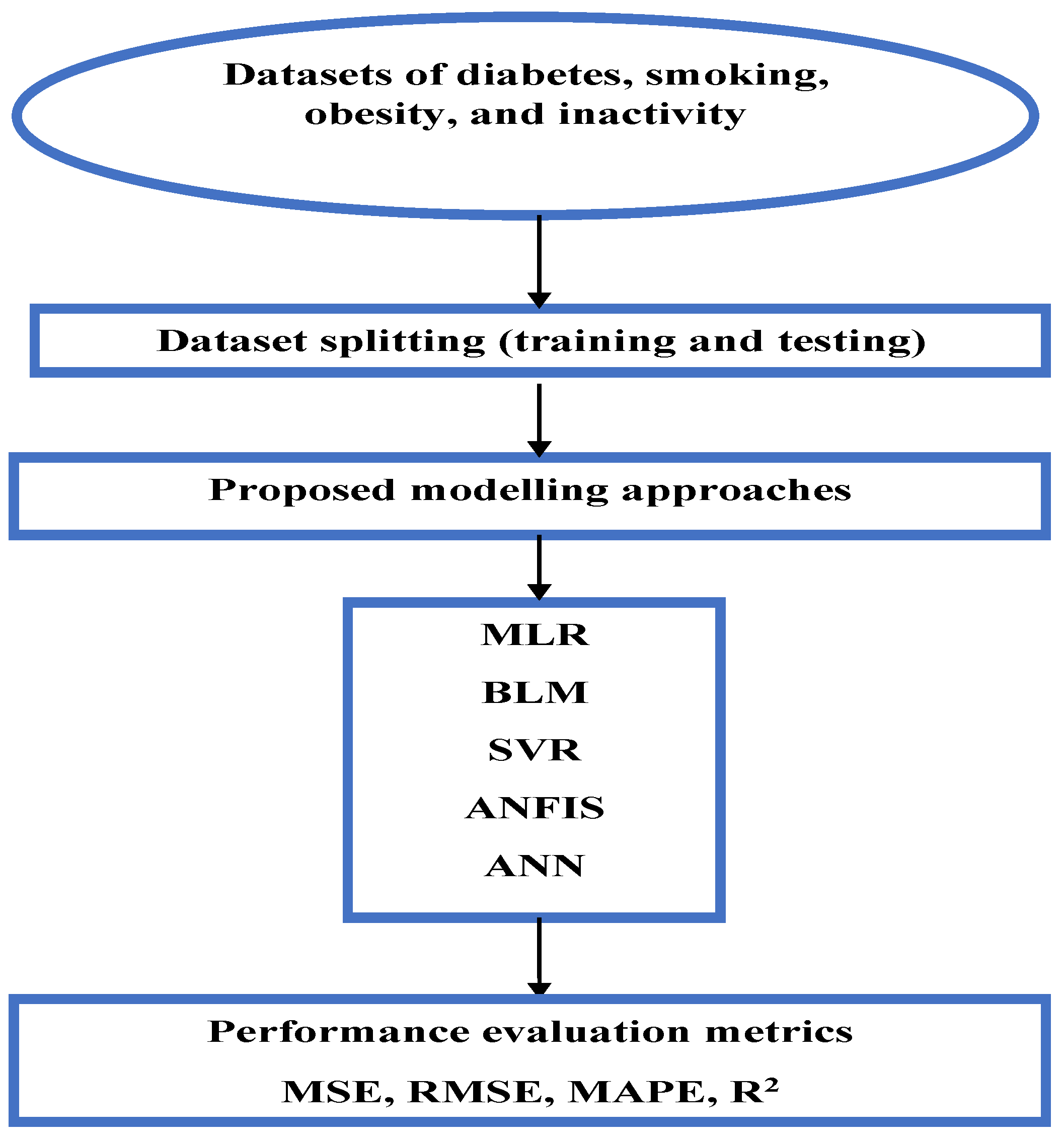
This section details the implementation of five regression-based machine learning models used to predict diabetes prevalence. Each model was trained on the training dataset and validated using the testing dataset. Model performance was evaluated using standard statistical metrics, including Mean Squared Error (MSE), Root Mean Squared Error (RMSE), Mean Absolute Percentage Error (MAPE), and the coefficient of determination (R²). Figure 1 illustrates the proposed workflow of this study.

Before training the models, we expected MLR and BLR to perform well if the data exhibited linear trends, while SVR with a linear kernel was anticipated to yield similar results. In contrast, ANN and ANFIS were expected to achieve higher accuracy in capturing nonlinear relationships. Among these, ANFIS was presumed to outperform the other models due to its integration of fuzzy logic, enabling it to handle complex patterns and uncertainties more effectively.

Multiple Linear Regression model: To establish this model in MATLAB, a constrained linear least-squares solver “lsqlin” with bounds or linear constraints was used to determine the regression positive coefficients for the MLR model using the training dataset. The optimisation toolbox lsqlin function was used as follows: coefficients = lsqlin (X, Y, [ ], [ ], [ ], [ ], lb, ub), where X is the independent (predictor) variables (gender, smoking, obesity, inactivity); Y is the dependent (response) variable (the prevalence of diabetes morbidity); and lb and ub are the constraints (equal to zeros and ones, respectively). The empty brackets ([ ]) in the lsqlin function mean that no linear inequality constraints (A, b) or linear equality constraints (Aeq, beq) are applied in the optimisation, so here we rely only on the bounds (lb, ub) to constrain the coefficients, without requiring any relationships (inequalities or equalities) between the variables. After calculating the model coefficients, the Multiple Linear Regression model is represented by the following equation:

$$Y=1+2.7\times {10}^{-10}{X}_1+0.2215X_2+0.1738X_3+0.0148X_4$$

(14)

where Y is the dependent variable (diabetes prevalence); $X_1$, $X_2$, $X_3$, and $X_4$ are the independent variables gender (men = 1, women = 0), smoking, obesity, and inactivity, respectively.

Bayesian Linear Regression model: To create this model the function (bayeslm) was used from the Econometrics Toolbox/Bayesian Linear Regression models in MATLAB (https://uk.mathworks.com/help/econ/bayeslm.html, accessed on 1 September 2024). Firstly, bayeslm was used to create a prior model object appropriate for predictor selection: p = 3; PriorMdl = bayeslm (NumPredictors p) This creates a diffuse prior model for the linear regression parameters, which is the default model type and identifies the number of predictors p. Then, the estimate function was applied to the prior model object, the predictors X, and the response Y (the training data) as follows: posteriorMdl = estimate (priorMdl, X, Y); By default, estimate returns a model object that represents the posterior distribution. Finally, to predict responses of Bayesian Linear Regression model, the forecast function was applied to the model object representing the posterior distribution as follows: forecast (posteriorMdl, x); where x represents the testing dataset.

SVR regression model: This model was applied using the fitrsvm tool in the Statistics and Machine Learning Toolbox [MATLAB, R2018a] (https://mathworks.com/help/stats/fitrsvm.html, accessed on 2 September 2024). As with the above trained models, the SVR model was trained using the training data, with the input values (independent variables) in the matrix and the target values (dependent variable) in the vector. SVR aims to find an optimal hyperplane by transforming the original feature space into a high-dimensional one utilising kernel functions. Some of the most popular kernel functions include linear kernel, polynomial function, Gaussian radial basis function (RBF), and hyperbolic tangent. In this study, the SVR model was trained with a default linear kernel, automatic hyperparameter tuning, and Sequential Minimal Optimisation. The default settings contain the Kernel Scale auto unit, which assigns a proper scale factor using a heuristic procedure based on subsampling with “Standardize” unit, which standardises each variable using mean and standard deviations, then the obtained SVR model can be used to predict diabetes prevalence using the test dataset.

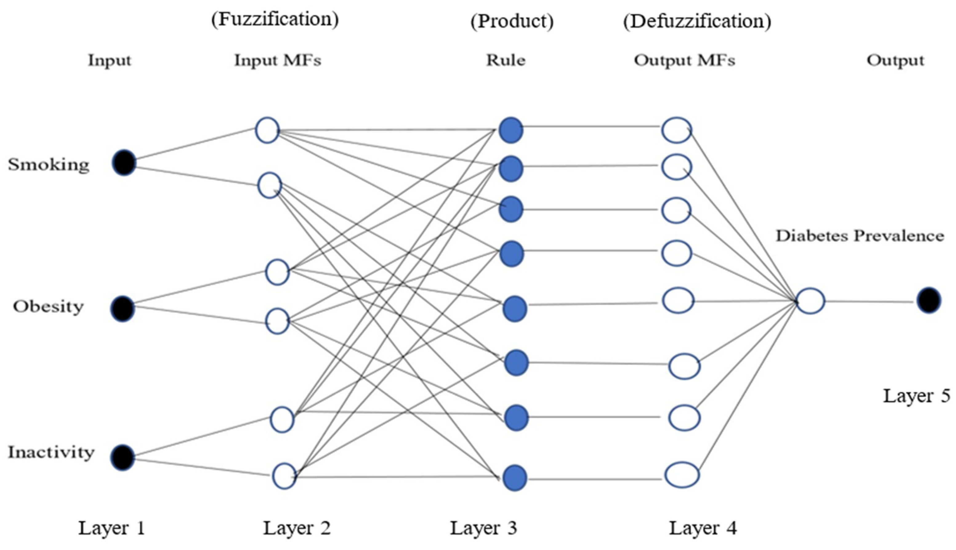
Adaptive Neuro-Fuzzy Inference System Model (ANFIS): This was modelled using the MATLAB Neuro-Fuzzy Designer app, determining the number and type of membership functions, and the optimisation method. To predict the prevalence of diabetes, the same training dataset that was used in the previous model was used to create an ANFIS structure with three inputs (smoking, obesity, and inactivity) and one output (diabetes prevalence) for both men and women. In order to train the ANFIS model, the number of membership functions was selected as 2 for each input; the Gaussian membership function was chosen for the type of function; and for the output variable, the type of membership function was linear. In addition, a hybrid method was implemented as the optimisation algorithm of the training, the error tolerance was set to 0, and the maximum number of epochs considered for training was set as 300. Figure 2 represents a typical ANFIS structure with three inputs, one output, and eight rules.

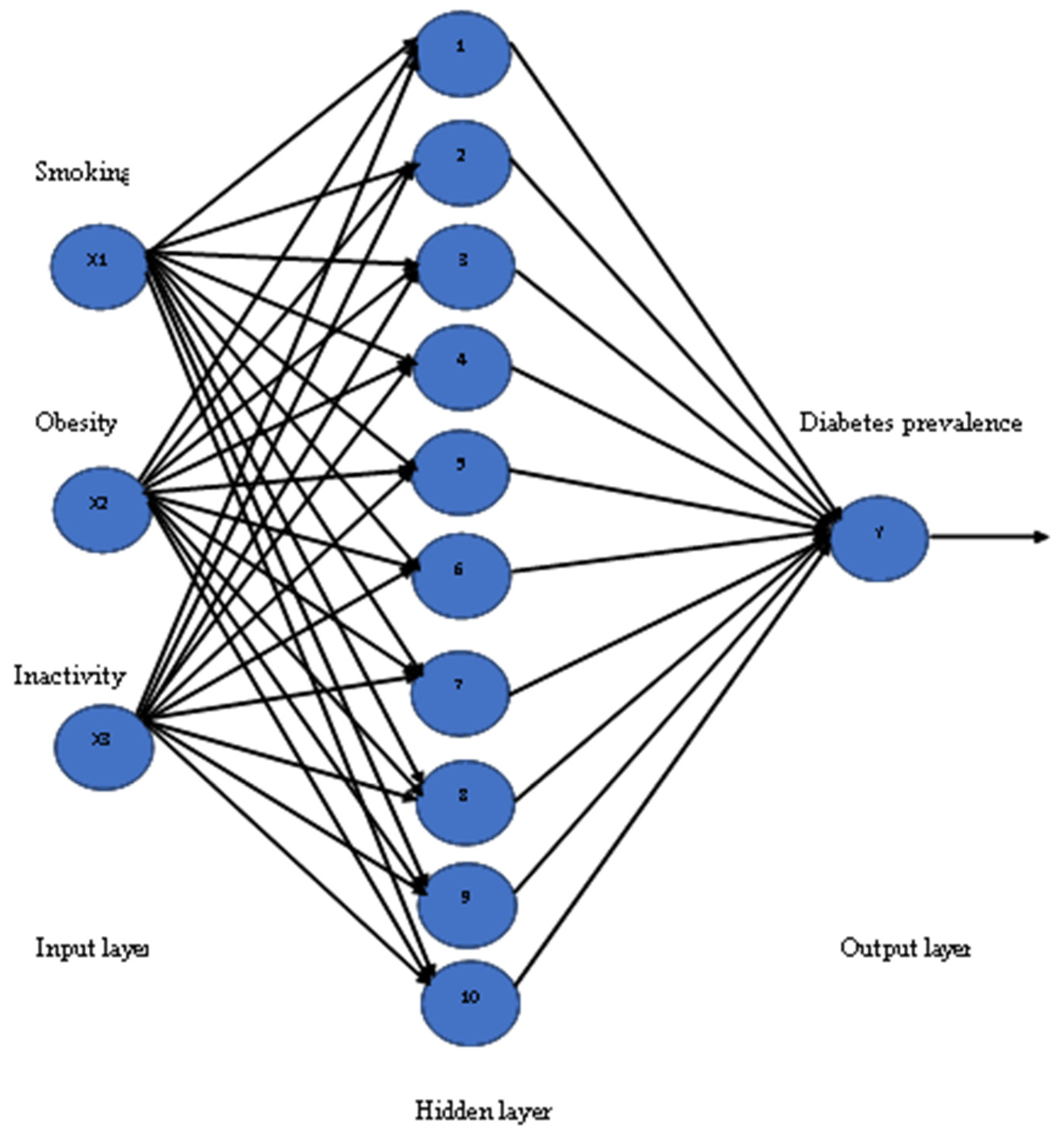
Artificial Neural Network (ANN): To apply this model a neural fitting tool (nftool) is used from the Neural Network toolbox in MATLAB, which is a two-layer feed-forward network with sigmoid hidden neurons and linear output neurons (fitnet). In this model, inputs are defined as X and targets as Y, with samples set in rows. The training dataset was used to create an ANN structure with three inputs (smoking, obesity, and inactivity) and one output (diabetes prevalence) for both men and women, and the number of neurons in the fitting network’s hidden layer was set to be 10. The training functions are varied and can be selected according to the type and size of a problem. To train the ANN model, the Levenberg–Marquardt algorithm was chosen, which is suitable for training small- and medium-sized networks, and it is an effective and fast training function. The structure of the ANN model has three input variables, with 10 neurons for the hidden layer, and one output variable, as seen in Figure 3. The training process of the Neural Network was allowed to be started by itself sufficiently until it was automatically stopped after a number of epochs, when it achieved the best validation performance.

5. Results

This section presents the findings from the regression models used to predict diabetes prevalence based on demographic and behavioural risk factors. The models were assessed using four key statistical evaluation metrics: Mean Squared Error (MSE), Root Mean Squared Error (RMSE), Mean Absolute Percentage Error (MAPE), and the coefficient of determination (R²). These metrics allowed for an objective comparison of the models’ performance and prediction accuracy.

Table 2. Total diabetes prevalence results for men and women (training data), 1999–2013.

	Men					Women
Year	MLR	ANFIS	ANN	SVR	BLM	MLR	ANFIS	ANN	SVR	BLM
1999	9.3	9.70	9.70	9.88	9.70	6.8	7.00	7.00	6.70	6.92
2000	9.6	9.80	9.70	10.03	9.81	7.0	7.12	7.26	7.08	7.23
2001	10.0	10.00	9.70	10.20	9.98	7.3	7.28	7.40	7.32	7.08
2002	10.4	10.20	9.70	10.43	10.21	7.5	7.50	7.50	7.55	7.49
2003	10.8	10.50	9.71	10.70	10.51	7.9	7.79	7.70	7.81	7.90
2004	11.2	10.90	9.80	11.04	10.88	8.3	8.14	8.14	8.18	8.23
2005	11.6	11.30	10.65	11.37	11.33	8.7	8.55	8.78	8.86	8.90
2006	12.0	11.80	11.90	11.78	11.81	9.1	8.99	8.99	9.20	9.25
2007	12.3	12.30	12.36	12.18	12.27	9.4	9.43	9.25	9.71	9.47
2008	12.7	12.70	12.69	12.56	12.71	9.8	9.84	9.69	10.13	9.77
2009	13.0	13.10	13.09	12.89	13.10	10.1	10.19	10.19	10.40	10.14
2010	13.2	13.40	13.35	13.17	13.38	10.3	10.48	10.53	10.45	10.13
2011	13.5	13.60	13.70	13.40	13.61	10.5	10.71	10.78	10.50	10.64
2012	13.7	13.80	14.09	13.58	13.80	10.6	10.88	10.88	10.52	10.63
2013	13.8	13.90	14.01	13.73	13.91	11.2	11.00	11.85	10.50	11.21

presents the regression modelling results for diabetes prevalence among men and women aged ≥25 years during the training period (1999–2013). The results show a steady increase in diabetes prevalence over time, with a higher prevalence among men than women. In men, diabetes prevalence increased from 9.7% in 1999 to 13.9% in 2013, reflecting an absolute increase of 4.2 percentage points (pp) and an annual increase of 0.3 pp. Similarly, the prevalence in women rose from 7% in 1999 to 11% in 2013, at the same annual increase of 0.3 pp. The performance evaluation metrics for the training data, shown in

Table 3. Statistical evaluation metrics results for all regression models for both men and women.

	Men				Women
	MSE	RMSE	MAPE	R2	MSE	RMSE	MAPE	R2
MLR	0.0420	0.2049	0.0150	0.9814	0.0247	0.1571	0.0139	0.9878
ANFIS	0.0013	0.0365	0	0.9994	0.0005	0.0239	0.0021	0.9997
ANN	0.0081	0.0899	0.0252	0.9964	0.0594	0.2437	0.0137	0.9705
SVR	0.0328	0.1810	0.0147	0.9855	0.0231	0.1520	0.0132	0.9885
BLM	0.0032	0.0564	0.0011	0.9986	0.0392	0.1980	0.0177	0.9806

, revealed that ANFIS achieved the best results, with RMSE = 0.04 and R² = 0.99 for men and RMSE = 0.02 and R² = 0.99 for women, indicating that ANFIS was highly accurate in modelling the observed trends, outperforming other regression techniques.

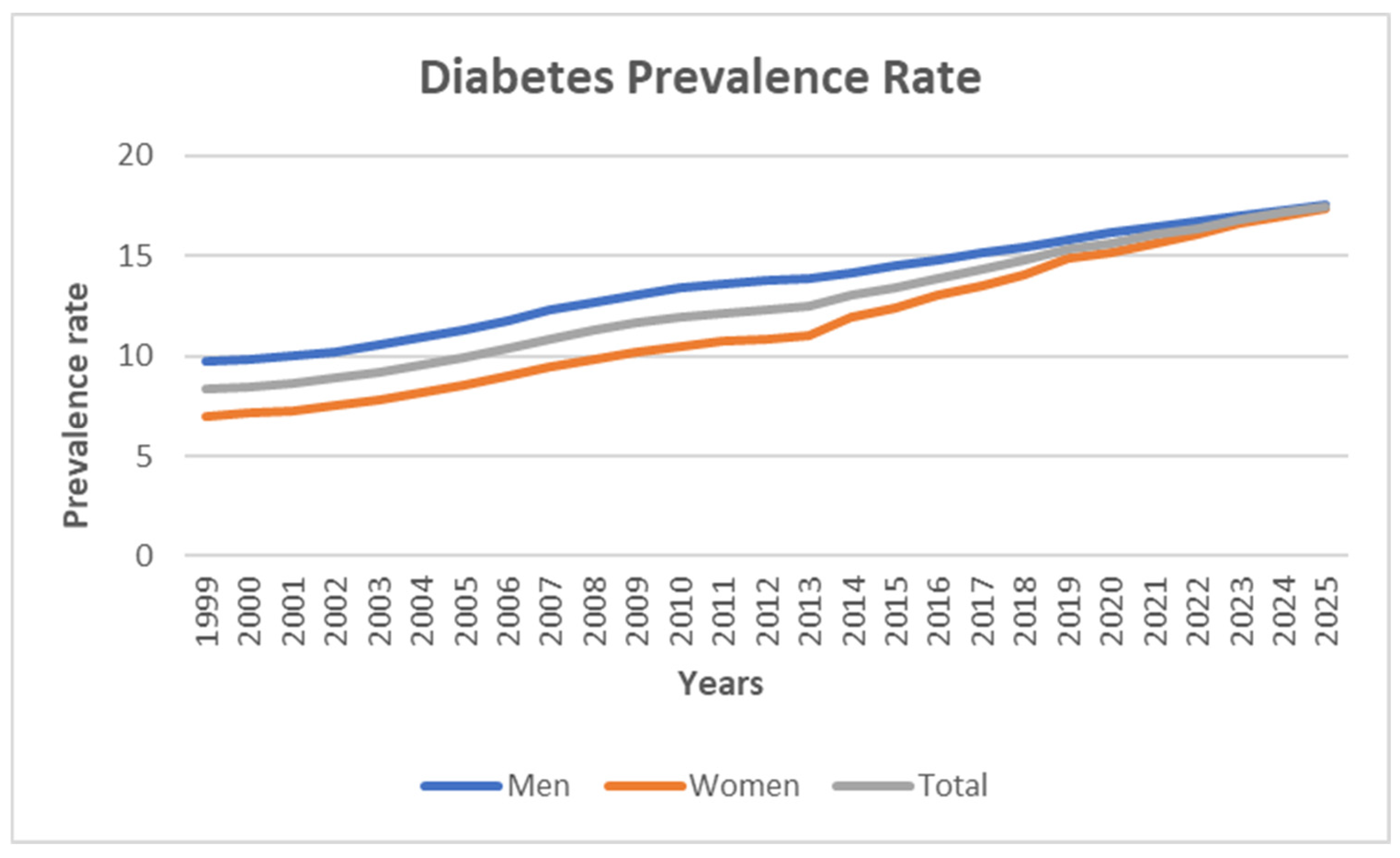
Using the test dataset (2014–2025), projections were made assuming the observed 1999–2013 trends continue.

Table 4. Total diabetes prevalence results for men and women (test data), 2014–2025.

	Men					Women
Year	MLR	ANFIS	ANN	SVR	BLM	MLR	ANFIS	ANN	SVR	BLM
2014	14.1	14.2	14.5	13.8	14.4	12.9	12.2	11.5	12.1	12.6
2015	14.2	14.4	15.1	13.9	14.7	13.4	12.8	11.7	12.4	13.1
2016	14.4	14.8	15.8	14.0	15.1	14.6	13.1	12.3	13.2	14.2
2017	14.6	15.2	16.6	14.1	15.5	15.1	13.8	13.1	13.5	14.6
2018	14.7	15.5	17.0	14.1	15.9	15.7	14.4	14.1	13.8	15.1
2019	14.9	16.0	17.7	14.2	16.3	16.8	14.8	15.5	14.2	16.1
2020	15.1	16.6	18.2	14.2	16.7	16.8	15.7	15.9	14.5	16.0
2021	15.2	17.1	18.6	14.3	17.1	17.3	16.4	16.4	14.8	16.5
2022	15.4	17.7	18.8	14.3	17.5	17.9	17.0	16.8	15.2	16.9
2023	15.5	18.3	18.9	14.4	17.9	19.0	17.4	17.0	15.9	18.0
2024	15.7	19.0	19.1	14.4	18.3	19.5	18.1	17.1	16.3	18.4
2025	15.9	19.6	19.2	14.5	18.8	20.1	18.7	17.2	16.6	18.9

presents these estimates, where the projected diabetes prevalence for men is expected to rise from 14.2% in 2014 to 17.6% in 2025, and for women it is projected to increase from 12.4% in 2014 to 17.3% in 2025. The low MSE and RMSE values across models further confirm the reliability of these projections, indicating that the models are able to make accurate predictions. Figure 4 illustrates the total estimated diabetes prevalence from 1999 to 2025 for both men and women, showing an upward trajectory in all cases.

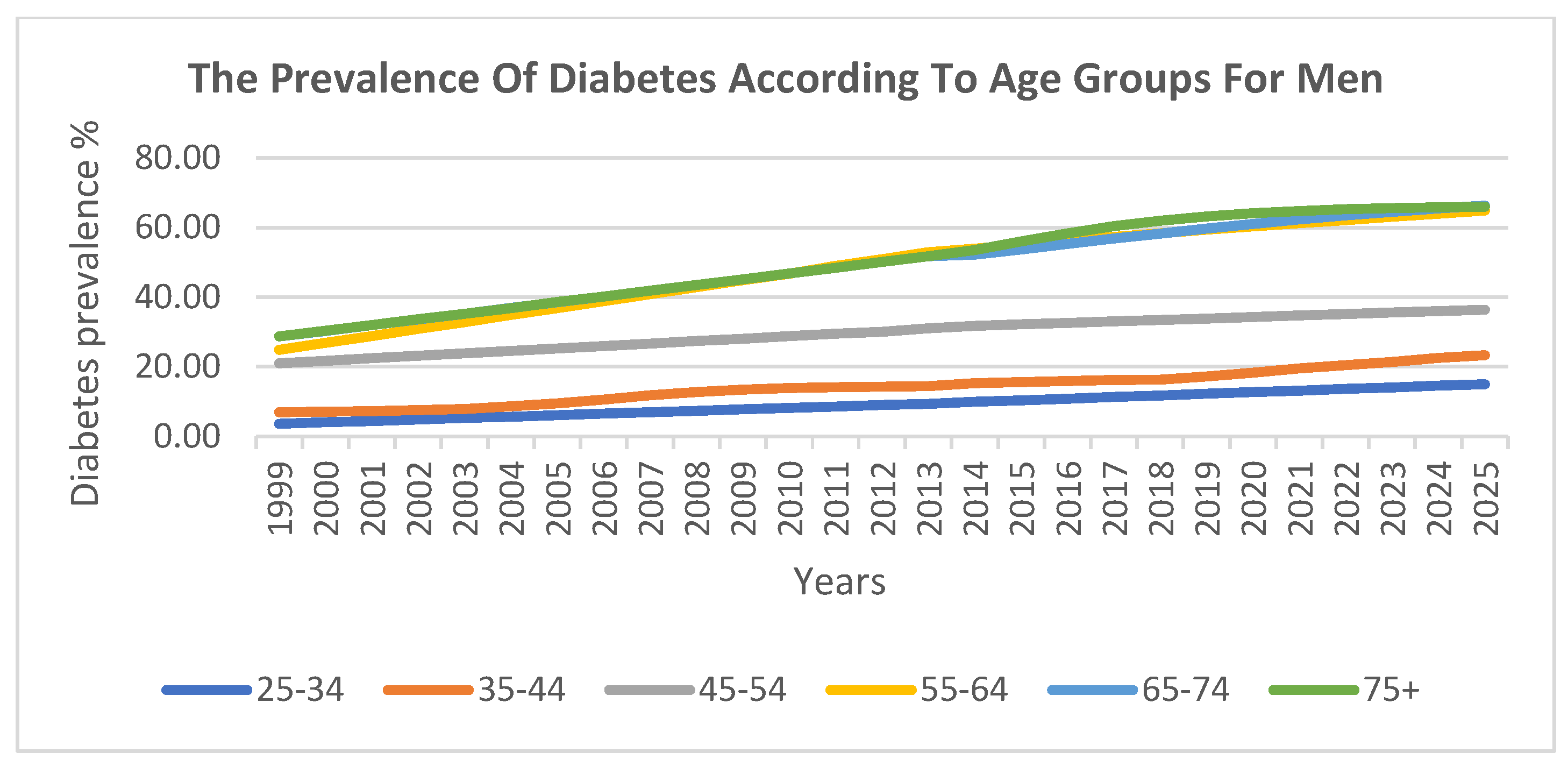
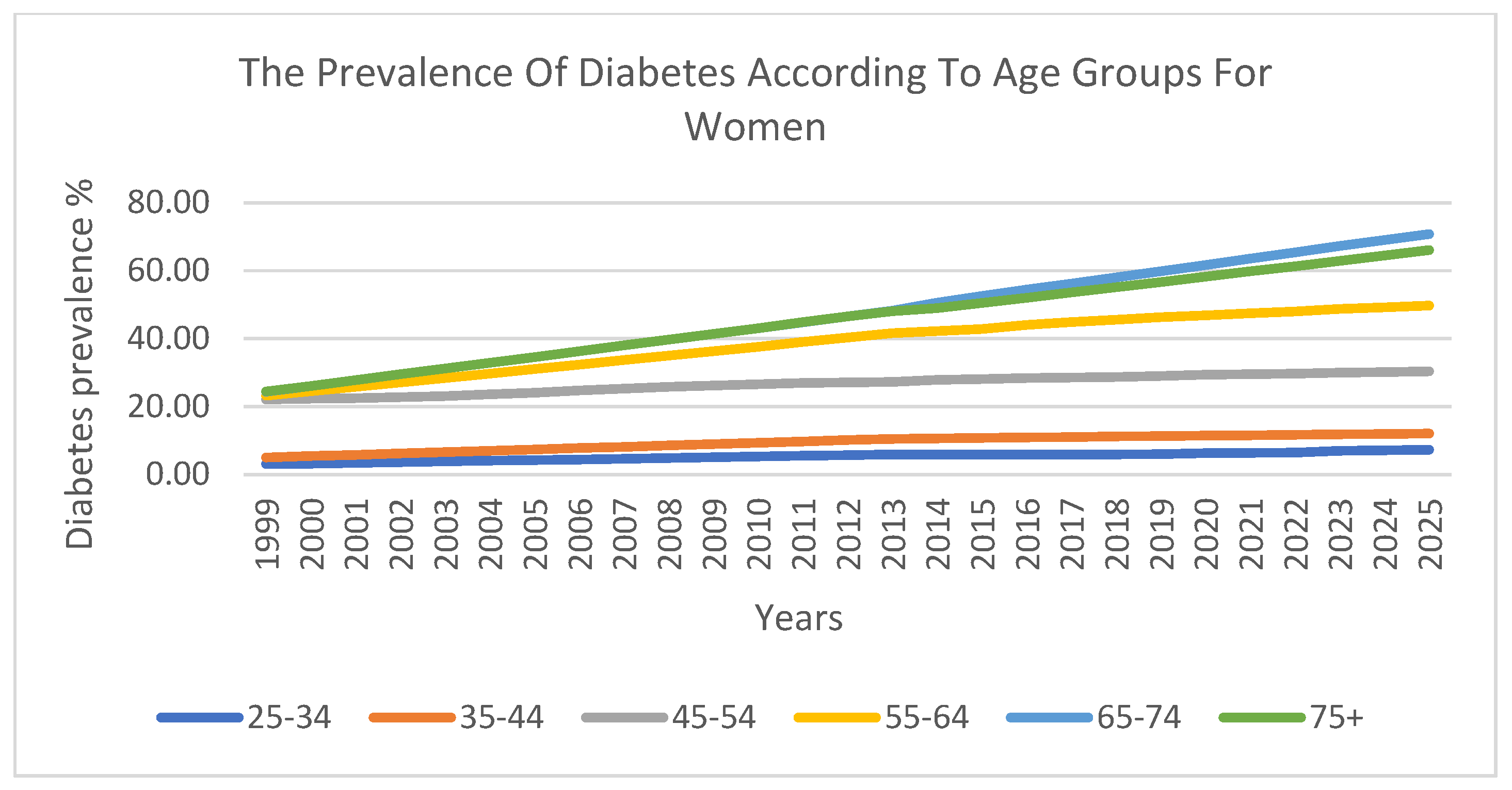
The prevalence of diabetes was also analysed across six ten-year age groups. The findings indicate that there was a lower prevalence in younger age groups, which steadily increased with age. The highest prevalence was observed among individuals aged 55–74 years. Figure 5 and Figure 6 visualise these trends across age groups for men and women, respectively, further confirming the strong correlation between age and diabetes prevalence.

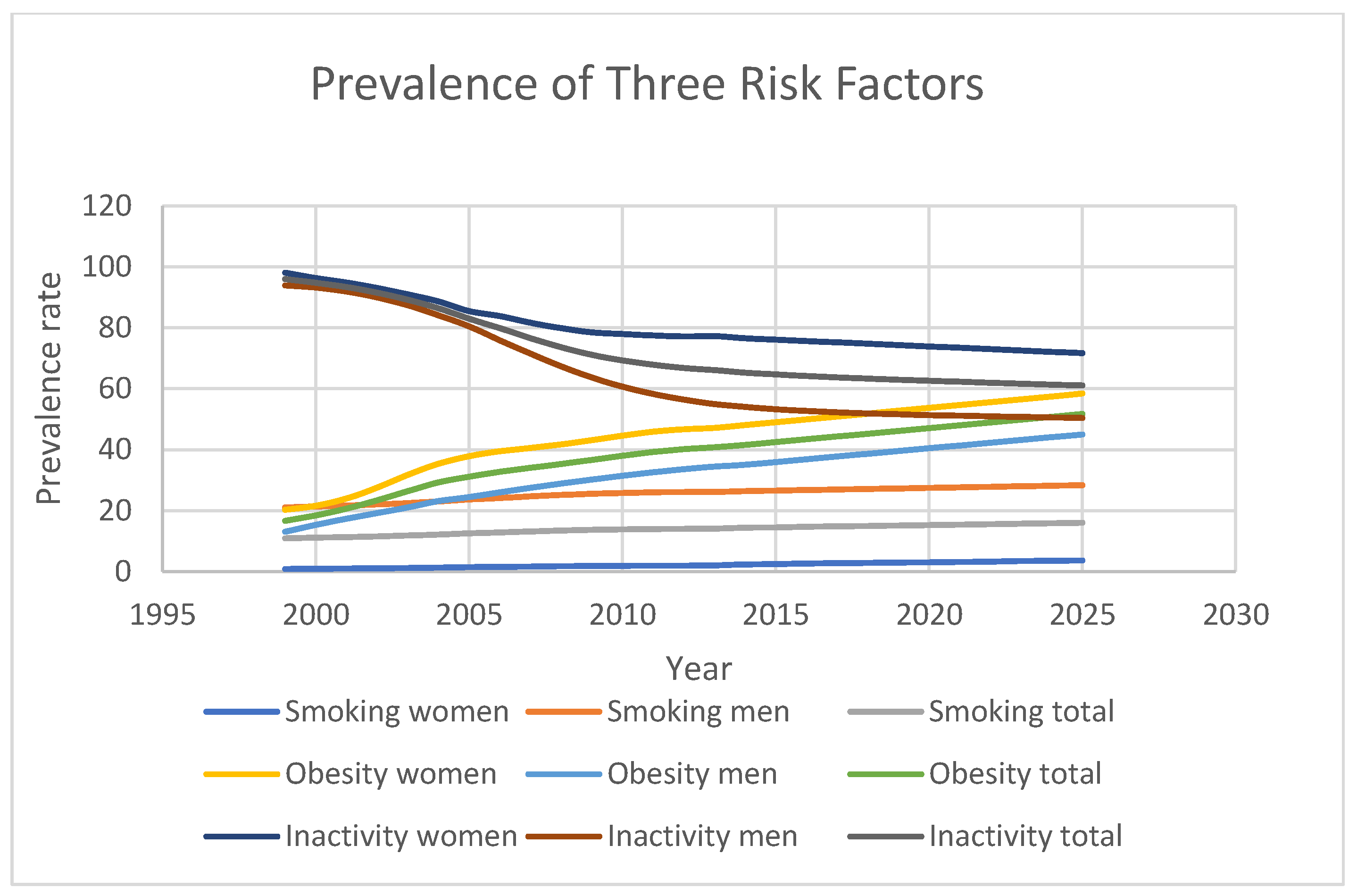
Figure 7 highlights the projected trends for behavioural risk factors associated with diabetes. Smoking prevalence is expected to increase from 11% in 1999 to 16.05% in 2025, while obesity rates will rise sharply from 16.7% to 51.7% over the same period. In contrast, physical inactivity is predicted to drop significantly from 96% in 1999 to 61.1% in 2025, although this percentage remains dangerously high. Furthermore, gender-based disparities in risk factor prevalence were observed. For instance, men had consistently higher smoking rates than women (21.1% vs. 0.9% in 1999; 28.4% vs. 3.7% in 2025), while women exhibited higher obesity prevalence (20.3% vs. 13.1% in 1999; 58.4% vs. 45% in 2025). Additionally, physical inactivity was more prevalent among women than men (98.1% vs. 93.9% in 1999; 71.7% vs. 50.5% in 2025).

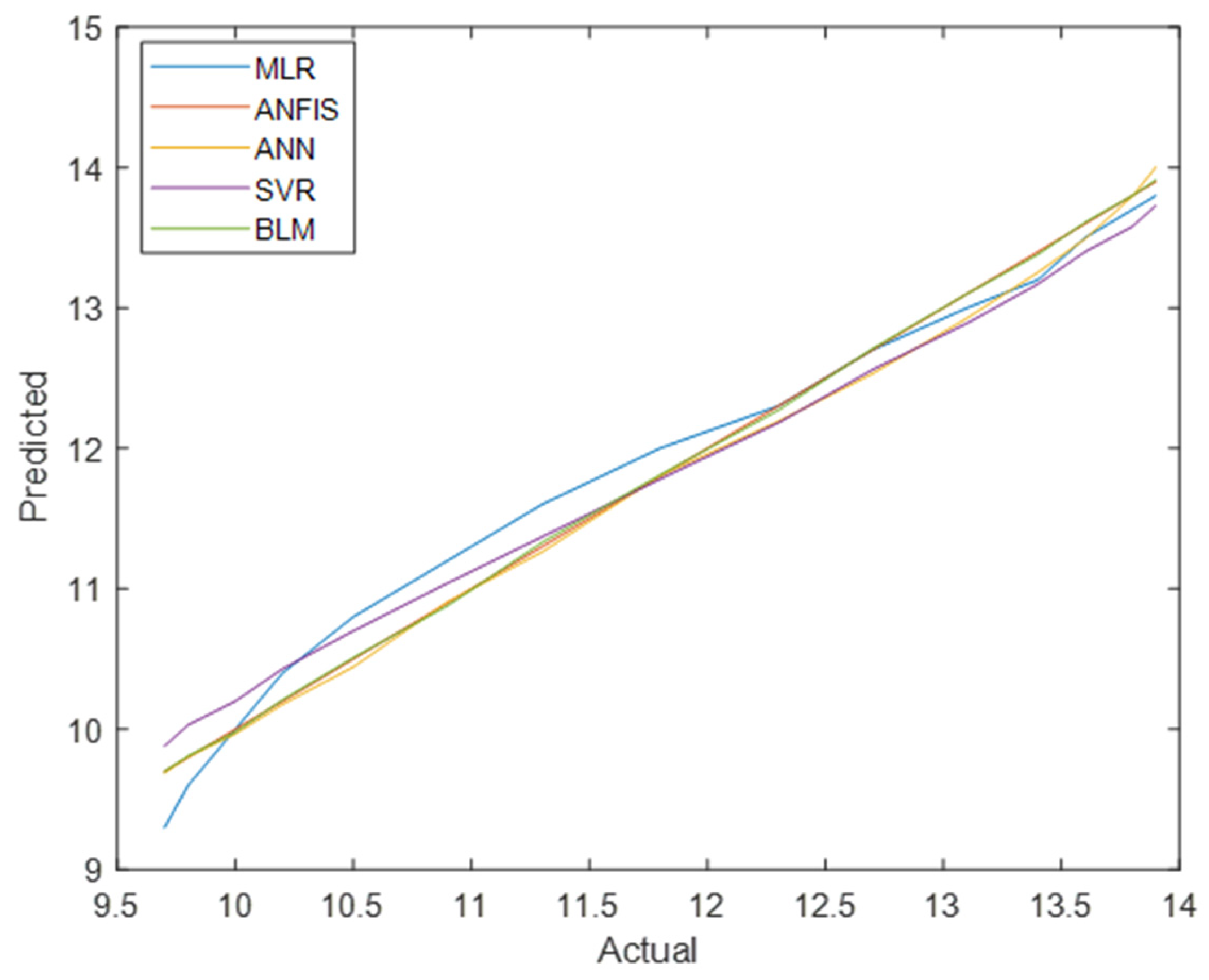
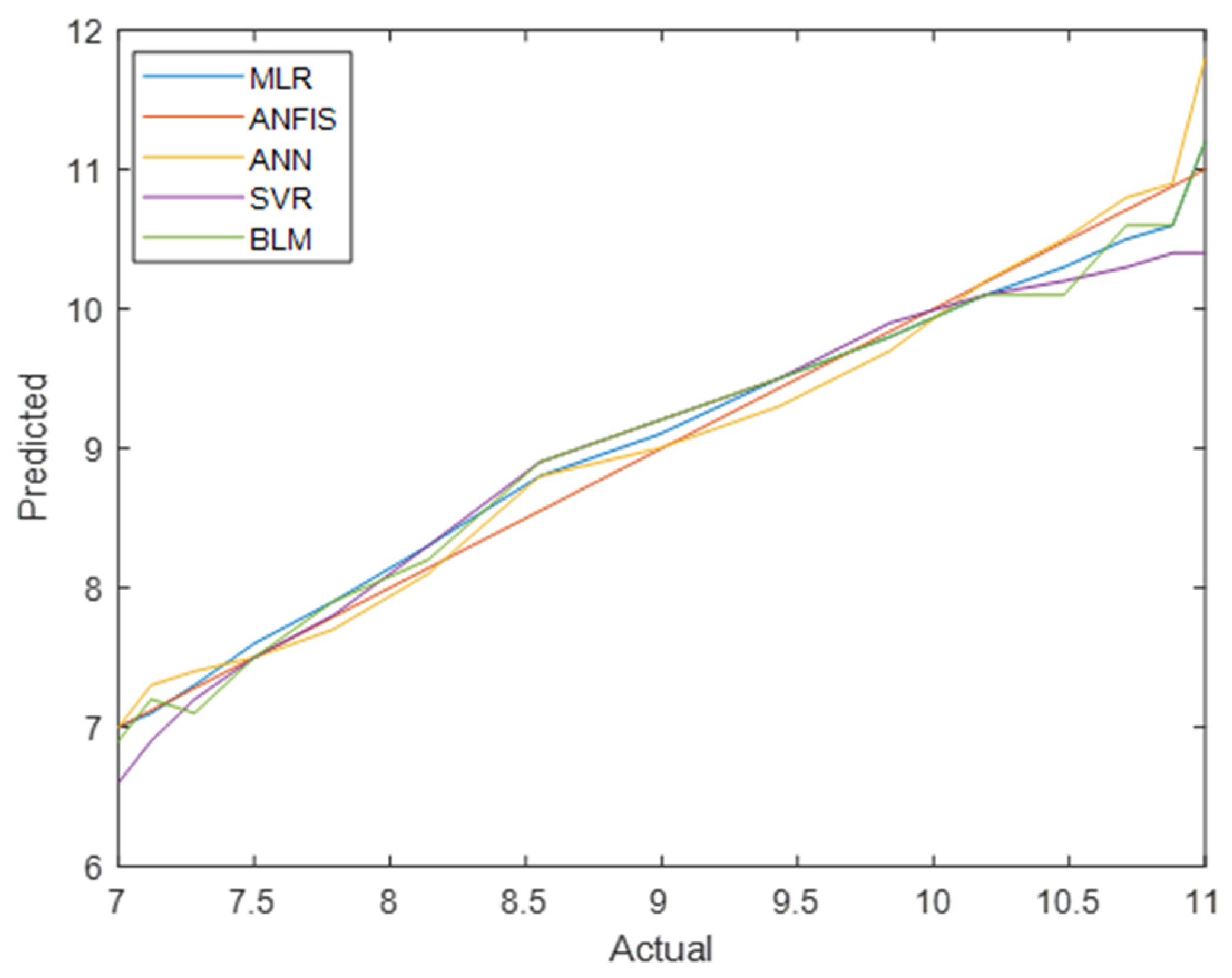
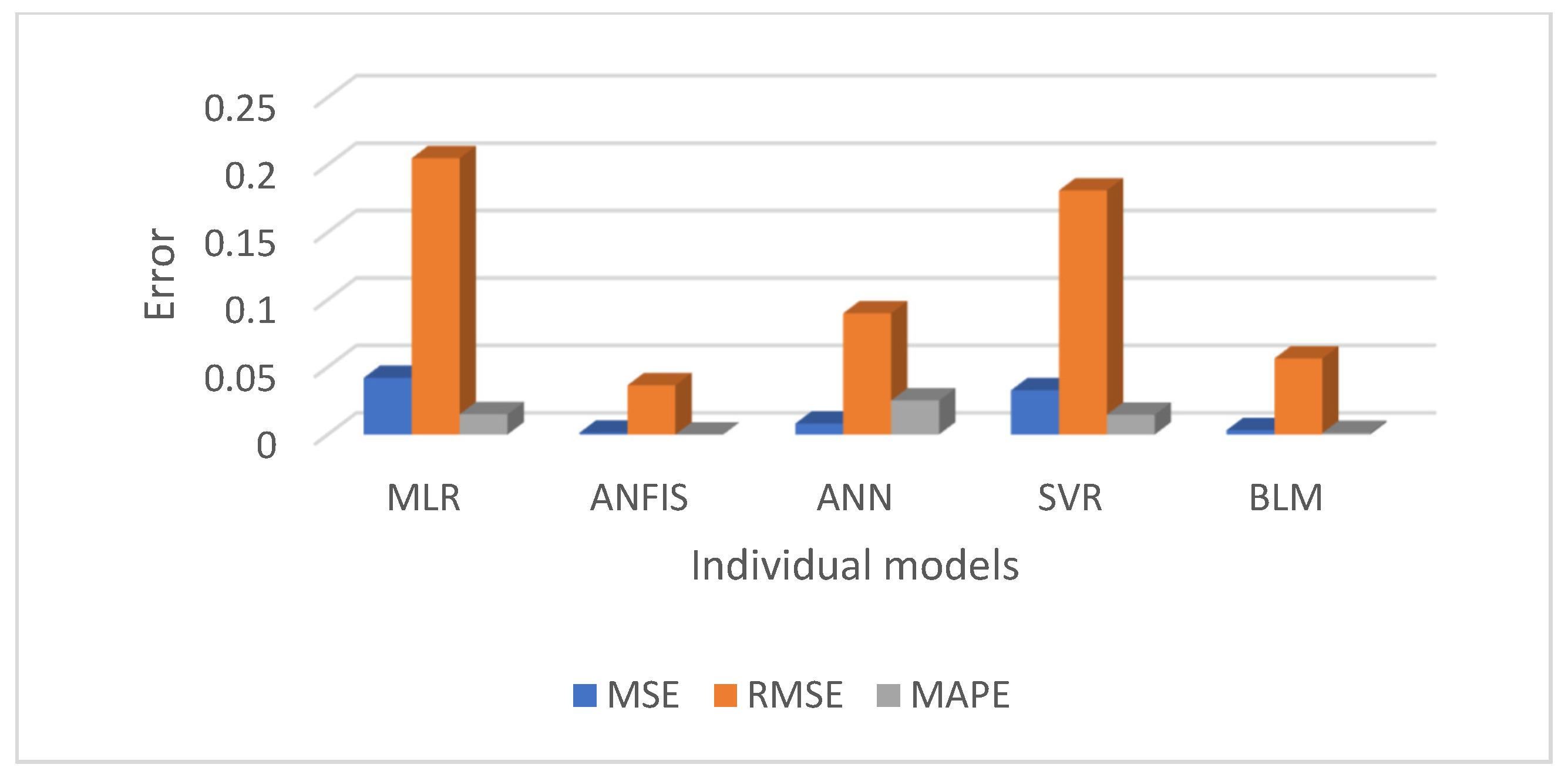
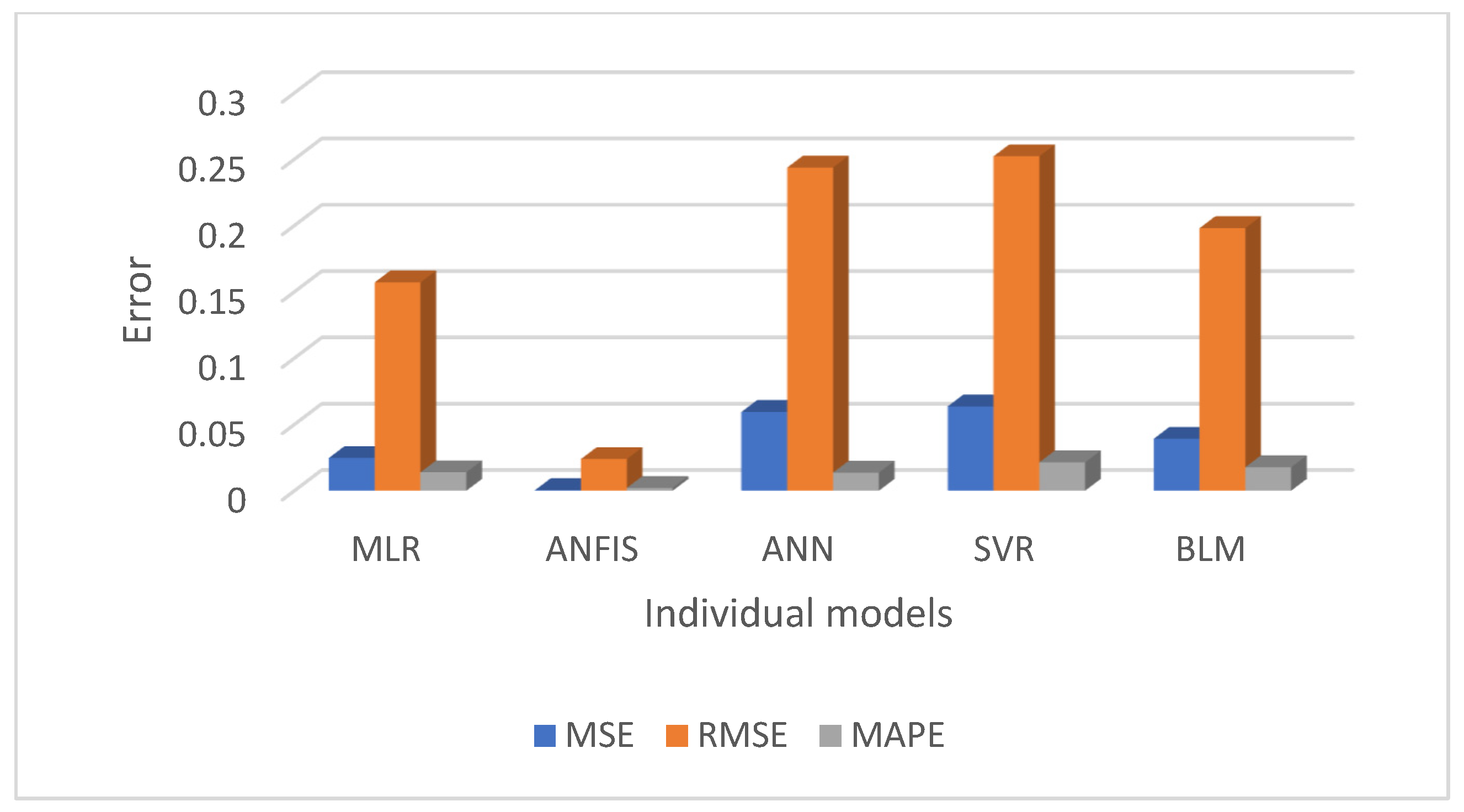
Finally, Figure 8 and Figure 9 compare the actual vs. predicted values for total diabetes prevalence in men and women across all models. ANFIS consistently produced the most accurate predictions, as shown by its superior performance metrics. Figure 10 and Figure 11 present a comparative analysis of all regression models, emphasising that ANFIS significantly reduces prediction errors for both the men’s and women’s datasets.

6. Discussion

This study evaluated and compared multiple regression-based machine learning models for predicting diabetes prevalence based on demographic and behavioural risk factors. The results highlight the strengths of various models and provide valuable insights into the future trajectory of diabetes prevalence. The performance of each regression model was summarised in Table 3, using evaluation metrics such as MSE, RMSE, MAPE, and R². Overall, the ANFIS model demonstrated superior predictive accuracy, achieving the lowest RMSE and the highest R² values for both the men’s and women’s training datasets. Specifically, ANFIS achieved RMSE = 0.04 for men and 0.02 for women, and R² = 0.99 for both groups, showcasing its remarkable ability to model diabetes trends with precision. As anticipated, SVR, with a linear kernel, yielded results similar to those of MLR, while BLR and ANN also displayed reasonably good performance. However, the ANFIS model consistently outperformed all other models, confirming our hypothesis that a hybrid approach would offer better predictive accuracy.

These findings indicate that ANFIS is the most effective model for predicting diabetes prevalence. Its ability to capture complex, nonlinear relationships within the dataset makes it particularly valuable for healthcare decision making, especially in predicting long-term trends. While the models provided good performance, certain models were better suited for specific datasets, underlining the importance of selecting the most appropriate models for different demographic groups.

The increasing prevalence of diabetes across all age groups is a concerning trend. As highlighted in the results, the highest rates of diabetes were found among individuals aged 55–74 years, with both men and women showing steady increases in prevalence over time. The findings also highlight gender-based disparities in the prevalence of diabetes, with men generally exhibiting higher rates of the disease but women often experiencing more severe health consequences. This underscores the importance of addressing gender-specific health strategies in diabetes prevention and management.

In addition to diabetes prevalence, this study also investigated the trends in behavioural risk factors, including smoking, obesity, and physical inactivity. The results show that while smoking and obesity are expected to increase over time, there is a promising decrease in physical inactivity. However, despite this improvement, the overall prevalence of inactivity remains uncomfortably high, indicating that public health initiatives must focus on increasing physical activity among the population. The gender differences in behavioural risk factors are also significant, with men exhibiting higher smoking rates and women showing higher obesity rates. These findings suggest the need for targeted interventions based on gender-specific patterns.

This study demonstrates significant strengths, such as the use of advanced predictive models and a well-structured dataset. However, there are certain limitations, including the reliance on self-reported data for behavioural variables, which may introduce bias. Future research could address these limitations by incorporating a more diverse dataset and additional predictors.

7. Conclusions and Future Work

This paper investigated the trends in diabetes prevalence in the Saudi adult population using historical diabetes data, along with smoking, obesity, and inactivity data as predictor variables, employing five different regression modelling techniques. Various evaluation criteria, including MSE, RMSE, MAPE, and R², were used to assess the performance of each model. The results showed that there was little difference in the performance of the models when using datasets for men and women. However, the ANFIS model consistently performed well in predicting the overall prevalence of diabetes for both men and women, as well as for each age group. For practical applications, we recommend the ANFIS model as a reliable and effective tool for diabetes prediction. However, this recommendation is based on data from the Saudi population, and further studies are needed to validate its performance in other populations. The findings also indicated that demographic factors (such as age and gender), as well as behavioural risk factors, significantly contribute to the increased prevalence of diabetes. Among these, smoking, obesity, and physical inactivity were identified as the most significant contributors.

For future research, it would be beneficial to explore the impact of integrating additional risk factors for diabetes in Saudi Arabia, such as diet and blood pressure. Additionally, considering non-modifiable risk factors, including family history and gestational diabetes, could further improve predictions. Expanding the range of risk factors could enhance the accuracy of diabetes prevalence predictions. Furthermore, investigating the application of machine learning techniques to predict the risk of diabetes-related complications, such as nephropathy, retinopathy, and cardiovascular diseases, could provide valuable insights. These efforts could not only help individuals with diabetes live healthier lives but also reduce the rising costs of healthcare.