Means and Issues for Adjusting Principal Component Analysis Results

Abstract

Background: Principal component analysis (PCA) is a method that identifies common directions within multivariate data and presents the data in as few dimensions as possible. One of the advantages of PCA is its objectivity, as the same results can be obtained regardless of who performs the analysis. However, PCA is not a robust method and is sensitive to noise. Consequently, the directions identified by PCA may deviate slightly. If we can teach PCA to account for this deviation and correct it, the results should become more comprehensible. Methods: The top two PCA results were rotated using a rotation unitary matrix. Results: These contributions were determined and compared with the original. At smaller rotations, the change in contribution was also small and the effect on independence was not severe. The rotation made the data considerably more comprehensible. Conclusions: The methods for achieving this and an issue with this are presented. However, care should be taken not to detract from the superior objectivity of PCA.

1. Introduction

Much of the data we handle consist of numerous measurement items, requiring multivariate analysis. Among the various methods available, principal component analysis (PCA) is particularly well-suited for scientific studies due to its limited methodological flexibility and high reproducibility [1,2,3,4,5,6,7,8,9]. The simplicity of PCA ensures that its results are consistent, regardless of the individual performing the analysis. This property is highly valuable in scientific research as it guarantees objectivity.

In PCA, we use singular value decomposition (SVD) to separate the matrix into unitary matrices (U and V) and a diagonal matrix D,

M = UDV*,

where V* denotes the conjugate transpose of V, and M represents the data to be analyzed, often centred or even scaled. The diagonal elements of D are sorted in descending order. Using this decomposition, the principal components (PCs) can be derived as follows:

Y = MV = UD and Z = M*U = VD

where the column vector of Y is PC for the samples and that of Z represents the PCs for the measurement items (e.g., PC1, PC2, etc.) [8]. Since U and V are unitary matrices, they satisfy the properties U*U = I and UU* = I. This ensures that the row and column vectors are orthogonal and have a Euclidean norm of 1. Specifically, the inner product of a vector with itself equals 1, while the inner product with other vectors equals 0, confirming orthogonality. As a result, the column vectors of Y and Z are also independent. These vectors can be interpreted as rotations of the original matrix M, with the unitary matrices defining the axes and the diagonal elements of D determining their lengths.

Since the diagonal elements of D are sorted, PC1, PC2, and subsequent components account for the decreasing proportions of the total data variance. PCA thus identifies common directions within M and summarizes them in order of their significance. This ability to effectively reduce the dimensionality of multivariate data is a key advantage of PCA.

The advantage of PCA as a scientific method lies in its objectivity. Due to the limited degree of choice involved in its application, the results remain consistent regardless of who conducts the analysis. Given that science is inherently a collaborative endeavour, it is essential that participants are interchangeable at all times and that the implications of the data are clear and accessible to all. While there are other methods of multivariate analysis, such as cluster analysis and multiple regression analysis, none appear to be as well suited to scientific research as PCA in terms of objectivity. For instance, cluster analysis is inherently less suitable for scientific purposes due to the abundance of options available, which can lead to varying results depending on the choices made. This is because cluster analysis typically presents only one possible interpretation of the data. Additionally, PCA can be viewed as an upwardly compatible method, as it is capable of revealing multiple regression analysis outcomes. Furthermore, PCA has the ability to condense a vast amount of information into a well-defined and interpretable form. To illustrate this, consider a study examining changes in the mammary glands of rodents during pregnancy and childbirth. This study involved dozens of sample measurements and a microarray analysis of tens of thousands of genes [8]. Despite the sheer volume of data, PCA facilitated a clear and concise summary, elucidating the directional trends associated with pregnancy and childbirth, as well as the relationships between individual genes.

However, one of the drawbacks of PCA is its lack of robustness. Even a single outlier can cause errors in SVD. Naturally, noise affects the results. It is common for the identified directions to be slightly off. For instance, group positions or individual Y values may deviate slightly from the axes due to rotation. Since experimental data inherently contain noise, it is expected that noise-sensitive PCA will exhibit such errors. In such situations, there may be a temptation to adjust PCA results or train PCA to correct rotations.

Accordingly, PCA now offers various options for data manipulation. One approach, for instance, involves reducing the dataset to be subjected to SVD by selecting it in a specific way [10]. Another involves altering the direction of rotation derived from SVD [11,12]. Both orthogonal and oblique rotations are available, each offering several methods. Naturally, these variations result in different solutions, thereby compromising the objectivity of PCA. This subjectivity arises because the outcomes depend on the analyst’s choices, which poses a significant challenge when analyzing scientific data. Oblique rotations, in particular, introduce a high degree of freedom, potentially leading to arbitrary results.

This study introduces a straightforward method to rotate data in relation to the two principal components while maintaining their orthogonality. The impact of such rotations on the original PCA results is evaluated in terms of the contributions of the principal components. The findings reveal that mild rotations do not significantly alter the results.

2. Materials and Methods

The test data used in this study were obtained from the practical training of students on a soil study. All calculations were performed using R (4.4.0) [13], and both the data and R code are provided as Supplementary Materials. Due to significant variability in the calcium data, the data were z-normalized for each item before applying SVD. Consequently, the centring point corresponded to the mean value of the data; these centring and scaling steps are among the few options available in PCA. The calculation method used for PCA is described in the Introduction. Additionally, since the number of measured items and the sample size differed considerably, I scaled the PCs by the square root of the sample size to facilitate biplots on a common axis [8], specifically $Y_{\mathrm{s}}=Y/\sqrt{n_{\mathrm{i}}}$, where n_i is number of items, and so on.

The angle of rotation, however, needed to be determined on a basis that was intuitive and easily understandable for all. In this case, an angle of 14 degrees was selected because it aligned the potassium (K) component of PC1 horizontally while simultaneously positioning the calcium (Ca) component of PC2 closer to the vertical axis. Alternatively, an averaging method could be employed to achieve an overall alignment of the components.

3. Results

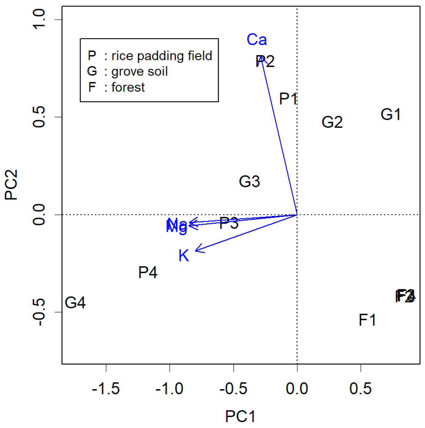
An example of a slight deviation of Z from the axes can be seen in Figure 1 (blue), which represents the PCA of data obtained from measuring substances in soil. Samples P1 to P4 were collected from points found downward, at 50 cm intervals from the surface of the padding field. Overall, soluble Na, K, and Mg appeared to have infiltrated the soil (P3, P4, G3, and G4), while less-soluble Ca remained near the surface (P1, P2, G1, and G2). In unfertilized forest areas, these materials were notably less (F1–F4). The measured items effectively differentiated these samples, demonstrating the impact of human activity on the land—increased calcium levels may alter surface soil, and cations that have penetrated underground could contribute to salinity. However, upon closer examination, the figure appears to be rotated counterclockwise by 14 degrees.

For example, when creating a two-dimensional plot using PC1 and PC2 for a matrix of four columns, these two column vectors can be rotated by taking the inner product of them with a rotation matrix, as follows:

$$R\left(\theta \right)=\left(\begin{array}{c}\begin{array}{cc} \cos \left(\theta \right)& \sin \left(\theta \right) \\ -\sin \left(\theta \right)& \cos \left(\theta \right)\end{array} \begin{array}{cc}0& 0\\ 0& 0\end{array}\\ \begin{array}{cc} 0 & 0 \\ 0 & 0 \end{array}\begin{array}{cc} 1& 0\\ 0& 1\end{array}\end{array}\right).$$

(1)

This is almost the identity matrix, but an alteration has been made in the upper left. This rotation matrix is unitary, so $R\left(\theta \right){R\left(\theta \right)}^{*}=I$, where I is the identity matrix. Consequently, if we rotate two columns of U, the adjusted U is $U_{\mathrm{a}}=UR\left(\theta \right)$. The resulting rotated matrix U_a is also unitary, as $UR\left(\theta \right) {\left\{UR\left(\theta \right)\right\}}^{*}=UR\left(\theta \right) {R\left(\theta \right)}^{*}{U}^{*}=U{IU}^{*}=I$. Since U and V are related as mirror images, if we rotate one column vector, we need to rotate the corresponding column vector by the same amount. From M = UDV*, we have

$$M=UR\left(\theta \right){R\left(\theta \right)}^{*}D(V{R\left(\theta \right){R\left(\theta \right)}^{*})}^{*}=U_a{R\left(\theta \right)}^{*}D{R\left(\theta \right)V}_a^{*}.$$

(2)

The matrix that is sandwiched by the two unitary matrixes,

$${R\left(\theta \right)}^{*}DR\left(\theta \right)=D_a,$$

(3)

is not necessarily a diagonal matrix, according to the twice rotations of D. Using D_a, Y_a = YR(θ) = MV_a = U_aD_a and Z_a = ZR(θ) = M*U_a = V_aD_a. Hence, the resulting column vectors of Y_a and Z_a are not necessarily independent. The degree of dependence depends on the rotation angle.

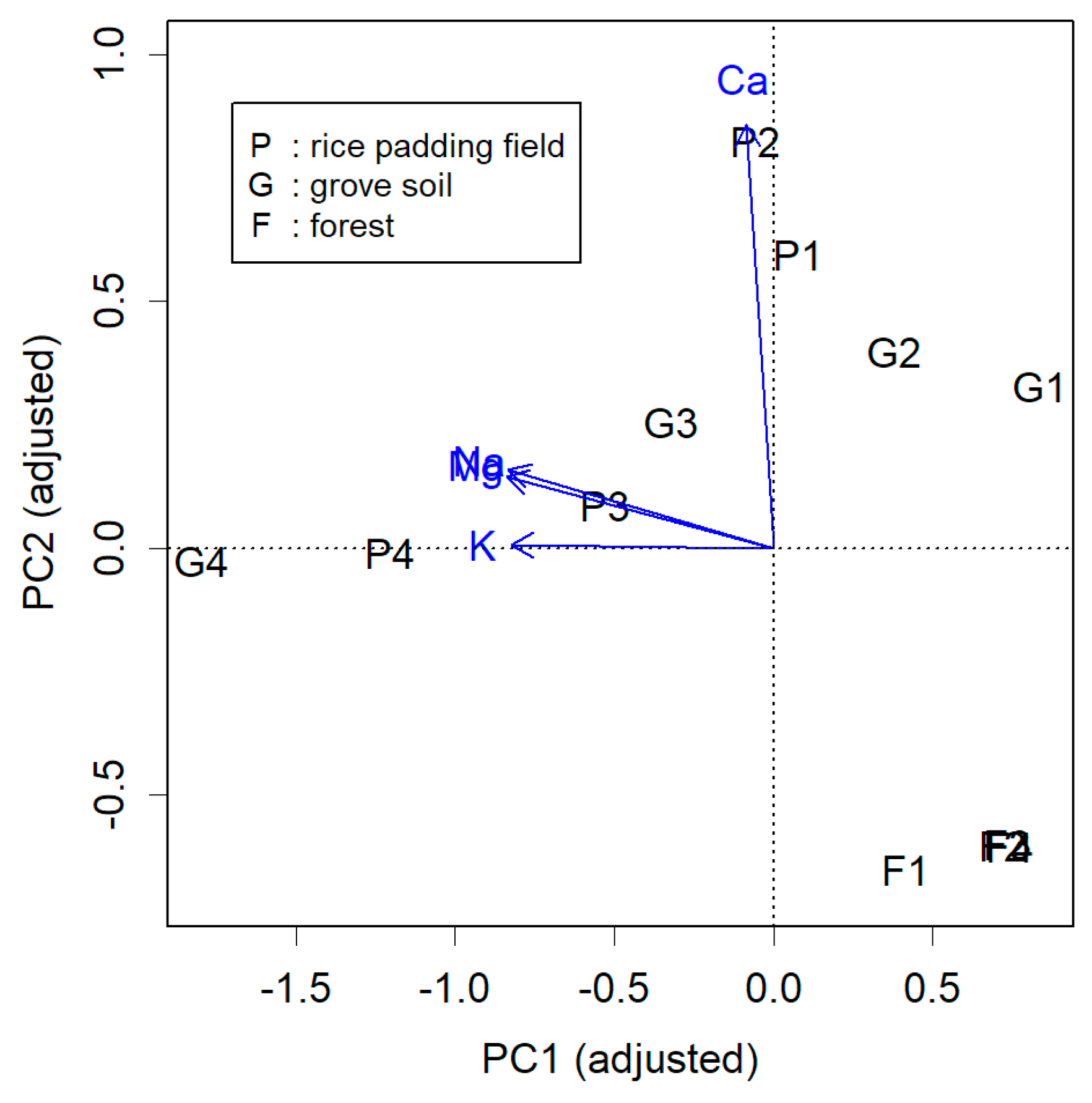
The actual result after rotating by 14 degrees is shown in Figure 2. Each item is now displayed closer to the axes (blue). Notably, the high calcium content in P1 and P2, as well as the abundance of soluble cations in G4 and P4, is more clearly visible. The question now is how much independence has been compromised. This becomes evident when examining the contribution of PC1.

Contributions are often derived from the diagonal elements of D. As D is a diagonal matrix, the contributions can be obtained from the component diag(D)/Σ(D). However, since D_a is not diagonal, we need to calculate the Euclidean distance using the squared sum of each column vector. The contribution is then given by the distance/total distance.

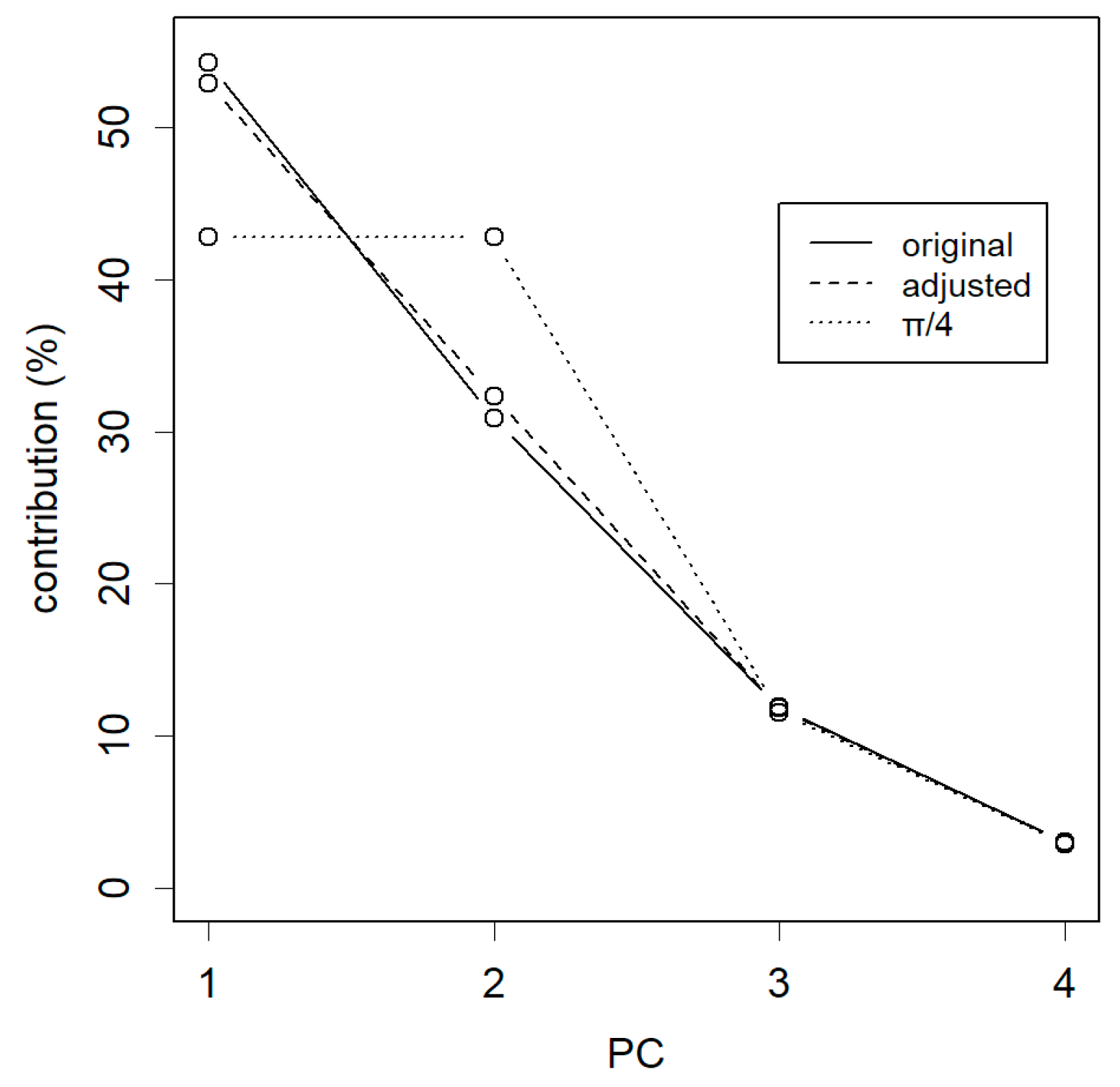
From the perspective of PCA, the goal is to collect contributions primarily from the top PCs. In the case of rotating by 14 degrees, the loss appeared to be relatively small (Figure 3, dashed line). In this context, the most significant change occurred when rotating by 45 degrees, π/4 (dotted line). At this point, PC1 completely lost its advantage over PC2, and both had equal contributions. In addition, of course, if rotated by 90 degrees, PC1 and PC2 would have effectively swapped places, and their contributions would have naturally switched as well. As the data’s dispersion remained preserved, the sum of all total distances was maintained regardless of the degree of rotations.

4. Discussion

In this analysis, PCA revealed two principal directions: PC1, which represented water-soluble ions that permeated the ground in a specific direction, and PC2, which represented a water-insoluble ion that remained on the surface. The samples were differentiated based on their respective depths within the soil, while forested areas that had not been treated were distinctly separated from the treated regions. The application of artificial rotation enhanced the clarity of this representation.

The results of the rotated PCA, albeit by a small angle, were more understandable. This somewhat compromises the priority of higher levels of PCs, but if the angle is not too large, the damage will not be too great. Understanding PCA plots can often be challenging, as PCA merely provides a summary, without revealing the specifics. Interpretation of the plot is left to the analyst. In this regard, enhanced readability could be highly appreciated. Notably, PCA is sensitive to noise. If this effect could be easily mitigated, this technique would be worth considering. To address this, it would be advisable to employ outlier detection methods provided by exploratory data analysis (EDA) [14,15]. This approach could potentially eliminate the need for artificial rotation, which would be a preferable outcome. In any case, introducing rotation complicates the process and reduces its objectivity. Unless there is a clear and compelling justification for its use, it would be more prudent to avoid it altogether.

It should be noted that this constitutes an active intervention by the analyst, potentially compromising PCA’s objectivity. The beauty of PCA lies in its impartiality. Diluting this aspect would be regrettable and might even lead to data manipulation. If such adjustments were made, it would be essential to keep the original, unadjusted plot available. This original information is also necessary for others to check whether a rotation was necessary. Alternatively, the rotated plot could serve as supplementary material for explaining the results. Although this analysis focuses primarily on the two main principal components (PCs), there may be instances where it is necessary to rotate subordinate PCs as well. However, this would further diminish the objectivity of the results. In such cases, it is recommended to present visual representations, such as those illustrated in Figure 3, to provide a clear and transparent depiction of the data.