Road Event Detection and Classification Algorithm Using Vibration and Acceleration Data

Abstract

Road event detection is critical for tasks such as monitoring, anomaly detection, and optimization. Traditional approaches often require complex feature engineering or the use of machine learning models, which can be computationally intensive, especially when dealing with real-time data from high-frequency vibration and acceleration sensors. In this work, we propose a Random Forest-based event classification algorithm designed to handle the unique patterns of vibration and acceleration data in road event detection for an urban traffic scenario. Our method utilizes vibration and acceleration data in three axes (x, y, z) to classify events in a robust and scalable manner. The Random Forest model is trained to identify patterns in the sensor data and assign them to predefined event categories, providing an efficient and accurate classification mechanism. Experimental results prove the effectiveness of our approach: it reaches an accuracy of 91.99%, with a precision of 80% and a recall of 75%, demonstrating reliable event classification. Additionally, the Area Under the Curve (AUC) score of 0.9468 confirms the model’s strong discriminative capability. Further, compared to a rule-based approach, our method offers greater generalization and adaptability, reducing the need for manual parameter tuning. While the rule-based approach attains a higher precision of 92%, it requires frequent adjustments for each dataset and lacks robustness across different road conditions.

1. Introduction

Detection of road events in urban traffic is essential for tasks such as safety monitoring, anomaly detection, and operational optimization [1,2,3,4,5]. Traditional classification methods often rely on direct feature extraction or complex models, which can be computationally intensive due to the need for high-resolution processing of large volumes of high-frequency vibration and acceleration data. This includes tasks such as filtering, transforming, and extracting features from multivariate time series data, which requires significant memory and computational power. In scenarios where input is restricted to specific vibration and acceleration patterns, achieving accurate and efficient classifications becomes a significant challenge [5,6].

Recent advances in machine learning, particularly Random Forest, have shown promise in improving classification accuracy without the need for extensive labeled datasets. Unlike deep learning models, which often require large amounts of training data, Random Forest can efficiently classify events using fewer labeled examples and can handle high-dimensional data with relative ease [7,8]. However, in urban traffic applications where data are dynamic and diverse, traditional Random Forest implementations may struggle to account for all possible event scenarios due to their dependence on static feature sets and the difficulty of capturing evolving patterns in vibration and acceleration data [9].

To address these challenges, we propose a novel Random Forest-based event classification algorithm that leverages vibration and acceleration data from three axes (x, y, z). Our method includes dynamic feature extraction tailored to road events, incorporating both statistical and frequency-domain features, which enhance the model’s ability to distinguish between diverse event types. By preprocessing the data with normalization and filtering, we reduce noise and ensure consistency, while the inclusion of windowed feature extraction captures temporal dependencies often missed by static implementations. This approach allows the model to adapt to varying urban traffic conditions, providing a robust classification of events such as vehicle movements, sudden stops, or irregularities in road conditions. Additionally, the model’s computational efficiency and simplicity make it suitable for real-time applications, directly addressing the limitations of traditional Random Forest methods in dynamic and diverse environments.

Our primary contribution lies in the effective integration of Random Forest for event classification, enabling robust, real-time detection with minimal computational overhead. Unlike traditional methods that struggle with high-dimensional sensor data, our approach efficiently processes vibration and acceleration signals without requiring large labeled datasets or complex preprocessing steps. Additionally, we demonstrate that Random Forest, despite being a simpler model compared to deep learning, offers high accuracy by handling data from multiple axes simultaneously. The experimental results validate the effectiveness of our method, showing that it outperforms other common classification techniques in terms of both classification accuracy and computational efficiency, offering a promising solution for road event detection in urban traffic and real-time event detection.

Random Forest

Random Forest is a group learning method that builds multiple decision trees to improve classification accuracy by aggregating the predictions of individual trees [10,11]. This technique is particularly effective in handling high-dimensional data and is less prone to overfitting compared to individual decision trees. The diversity of trees is achieved by training each tree on a random subset of the data, both in terms of the samples (bagging) and the features used for splitting at each node.

For event classification in road event detection, Random Forest offers a robust solution to identify patterns in vibration and acceleration data. The algorithm begins by creating multiple decision trees, each trained on a random subset of the data. Each tree makes a prediction based on the input features, and the final classification is determined by the majority vote of all trees in the forest. This process enables the model to handle noisy, high-dimensional sensor data and to classify events accurately without requiring extensive feature engineering.

The strength of Random Forest lies in its ability to reduce the risk of overfitting by aggregating the results of many decision trees, each of which captures different aspects of the data. Furthermore, it is computationally efficient, making it suitable for real-time applications in road event detection. The robustness of the model also ensures that it can adapt to the variability in sensor data across different urban environments, providing reliable event detection even in the presence of noise or inconsistencies in the data.

In addition, Random Forest can handle both numerical and categorical data, making it highly versatile for multi-modal sensor inputs, such as vibration and acceleration data. This capability improves its performance for classifying diverse events in complex systems, where the patterns of sensor data can vary greatly depending on factors such as road conditions, vehicle types, and driving behavior [12].

2. Related Works

The field of road event classification has seen significant advancements, particularly with the increasing use of machine learning models to handle complex, high-dimensional sensor data. Thus, deep learning-based methods, such as convolutional neural networks (CNNs), have shown promise in learning intrinsic patterns and classifying road events [13,14,15]. Although such methods demonstrate the potential of deep learning to manage complex, high-dimensional data, they often require extensive labeled datasets and significant computational resources.

In contrast, traditional feature-based methods, such as statistical feature extraction and wavelet transforms, continue to be relevant for certain applications due to their interpretability and lower computational cost [16]. These techniques rely on manually constructed features to identify specific patterns in vibration data. However, their performance may degrade in environments with overlapping or unpredictable event characteristics, where the variability of sensor data challenges the effectiveness of handcrafted features.

More recently, researchers have explored the use of ensemble learning methods, including Random Forest, to address some of these limitations. Random Forest offers a robust solution to classification tasks by aggregating predictions from multiple decision trees, making it less sensitive to overfitting and more effective in handling noisy and high-dimensional data. For example, authors of ref. [17] demonstrated that Random Forest could achieve high precision in classifying events from vibration and acceleration data, outperforming traditional methods and offering a more efficient solution than deep learning models for real-time applications.

In a similar trend, Celaya-Padilla et al. [6] proposed the use of a genetic algorithm to detect speed bumps, utilizing the characteristics of the accelerometer. Their approach demonstrated the potential of heuristic search techniques, such as genetic algorithms, to optimize feature selection for classification tasks. By combining genetic algorithms with sensor data, their method improved the accuracy and robustness of road event detection, especially in challenging environments with noisy and variable sensor data. This highlights the versatility of ensemble learning and optimization algorithms in enhancing the performance of event detection systems.

Sensor fusion techniques have also been widely explored to enhance classification accuracy. For example, refs. [18,19,20,21,22] highlighted the benefits of combining vibration data with accelerometer and gyroscope input to improve robustness and reduce classification errors. By merging data from multiple sensors, these hybrid methods leverage the complementary strengths of each sensor modality, improving overall performance in noisy, dynamic environments. Our approach similarly utilizes sensor data from multiple axes of vibration and acceleration to improve event classification accuracy.

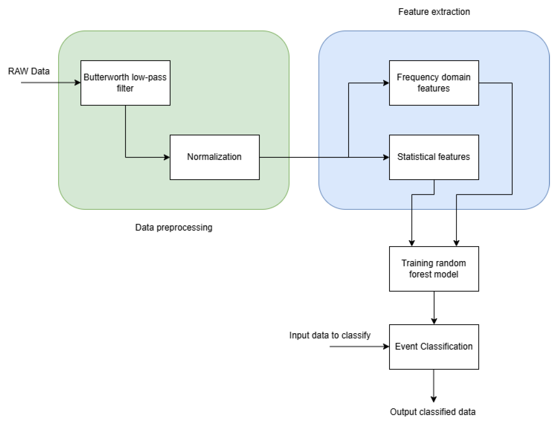
3. The Proposed Algorithm

An overview of the proposed event classification algorithm is illustrated in Figure 1. The algorithm uses vibration and acceleration data to identify patterns corresponding to various events, ensuring high accuracy and computational efficiency. Designed to process high-frequency sensor signals, it extracts key features that inform classification decisions in real time. The algorithm consists of the following main steps:

• Data Preprocessing: Collect vibration and acceleration data from the three axes (x, y, z). Normalize and segment the raw sensor data into time windows, each representing a distinct observation for classification.
• Feature Extraction: Extract relevant features from preprocessed data, such as statistical metrics (mean, variance, skewness, kurtosis) and frequency domain features (e.g., spectral entropy, power spectral density).
• Model Training: Train a Random Forest model using the extracted features as input. Each decision tree in the forest is trained on a random subset of the data and the final classification is based on the majority votes of the trees.
• Event Classification: Use the trained Random Forest model to classify incoming sensor data into predefined event categories (e.g., vehicle movements, sudden stops, irregularities). Although the main core of the Random Forest algorithm remains unchanged, we introduce several optimizations for road event detection using vibration and acceleration data. These modifications improve the efficiency, robustness, and applicability of the model in real-time environments.
  • Feature Engineering and Selection: To improve classification accuracy and computational efficiency, we apply a structured feature engineering process. First, we pre-process the raw sensor data by applying a Butterworth low-pass filter to remove high-frequency noise and normalize the signals to ensure consistency across different sensor readings. Then, we extract both statistical features (mean, variance, skewness, kurtosis) and frequency domain features (spectral entropy, power spectral density) to capture relevant patterns in the data. This set of features improves the ability of the Random Forest classifier to differentiate between different road events.
  • Hyperparameter Tuning: To optimize performance, we fine-tune the hyperparameters of the Random Forest model, adjusting the number of trees ($N_T$), the maximum tree depth, and the minimum samples required for a split. This tuning process, performed using cross-validation, ensures a balance between model complexity and generalization capability. The results of different hyperparameter configurations are analyzed in Section 5.
  • Class Balancing Strategy: Road event datasets are inherently unbalanced, as normal driving conditions occur more frequently than anomalies such as potholes or sudden braking events. To mitigate this issue, we apply a class weighting strategy that increases the importance of underrepresented event types during training. This approach prevents the model from being biased towards predictions of the majority class, ensuring better detection of rare but critical road events.

These optimizations make the Random Forest algorithm more suitable for real-time road event detection, balancing accuracy, computational efficiency, and robustness to sensor variations. Future work may explore additional optimizations, such as multimodal sensor integration and deep learning integration, to further enhance classification performance.

3.1. Data Preprocessing

To process the vibration and acceleration data for event classification, we first segment the raw sensor data into smaller, meaningful time windows. Each time window represents a distinct observation that is then used for feature extraction. This ensures that we focus on the most relevant data for event detection while minimizing computational complexity.

The process begins by collecting vibration and acceleration data from the three axes (x, y, z). The raw data are then preprocessed to remove noise and normalize the signals, ensuring that the features extracted from the data are on a comparable scale. This preprocessing step is crucial to achieving accurate and reliable classification results.

The pre-processing steps include:

• Noise Removal: The raw sensor data are filtered using a low-pass filter to remove high-frequency noise. This is achieved by applying a Butterworth low-pass filter, which is preferred due to its maximally flat frequency response in the passband and a smooth transition to the stopband. This helps eliminate unwanted high-frequency signal components that may interfere with the classification process. The equation for the Butterworth filter is given by

  $$H\left(s\right)={\displaystyle \frac{1}{1+{(s/{\omega }_c)}^{2n}}}$$

  (1)

  where ${\omega }_c$ is the cutoff frequency, n is the filter order, and s is the complex frequency. The filter removes components of the signal above the cutoff frequency, effectively reducing high-frequency noise.
• Normalization: The signals are normalized to a range between 0 and 1 to ensure consistency and prevent any bias caused by different magnitudes in the raw data. Normalization ensures that all features contribute equally to the classification process. Normalization is performed using Min–Max scaling, which is defined as

  $$S_{\mathrm{normalized}}={\displaystyle \frac{S-min\left(S\right)}{max\left(S\right)-min\left(S\right)}}$$

  (2)

  where S is the raw signal and $S_{\mathrm{normalized}}$ is the scaled signal. Min–Max scaling is chosen because it preserves the original distribution of the vibration and acceleration data while ensuring that all features are within a fixed range. Unlike Z-score normalization, which assumes a Gaussian distribution, Min–Max scaling is more suitable for this dataset, where sensor values exhibit skewed distributions due to road anomalies and sudden accelerations. This approach prevents large-magnitude signals from dominating the model while maintaining interpretability across different sensor readings.

Algorithm 1 illustrates the steps involved in the preprocessing process. This ensures that the data are cleaned, normalized, and segmented appropriately before proceeding to the feature extraction phase.

Algorithm 1: Data Preprocessing

1: Input: Raw vibration and acceleration dataset D  2: Output: Processed feature vectors $F_k$ for each time window $W_k$  3: Preprocess the raw data D  4:    1. Apply low-pass filter to remove high-frequency noise:  5:       For each signal $(vibratio{n}_x,vibratio{n}_y,vibratio{n}_z,acceleratio{n}_x,$$acceleratio{n}_y,acceleratio{n}_z)$:  6:          Apply a Butterworth low-pass filter with a cutoff frequency of 20 Hz  7:          Use filter equation:  8:             Filtered signal = butter_filter(raw_signal, cutoff_frequency = 20)  9:    2. Normalize the signals: 10:       For each signal $S_i$ in D (where $S_i$ represents vibration or acceleration data): 11:          Normalize the signal using Min-Max scaling: $$\begin{array}{c}\hfill \mathrm{Normalized}\mathrm{signal}={\displaystyle \frac{S_i-\min \left(S_i\right)}{\max \left(S_i\right)-\min \left(S_i\right)}}\end{array}$$ 12:    3. Segment the data into time windows $W_k$ for $k=1,2,\dots ,K$: 13:       Define window size: $window\_size=1\sec \mathrm{ond}$ 14:       For each signal $S_i$, segment into $W_k$ (overlapping windows or non-overlapping depending on the use case): 15:          For each window $W_k$ of $S_i$: 16:             Store the segmented data as $W_k$ 17:    4. Return the set of time windows $W_k$ for further processing.

The cutoff frequency of 20 Hz was chosen to focus on the dominant frequency components associated with road events, as vibrations and accelerations caused by such events typically occur below this threshold. The window size of 1 s balances capturing sufficient temporal context while maintaining computational efficiency for real-time processing.

3.2. Feature Extraction

After the raw data are preprocessed, the next step is to extract relevant features that aid in the classification process. The goal of feature extraction is to represent the raw sensor data in a form that captures the underlying patterns of different events (e.g., speed bumps, potholes, sudden brakings) in a compact and meaningful way.

To extract features, we divide each preprocessed time window $W_k$ into statistical and frequency domain features. Statistical features provide information on the central tendency and dispersion of the data, while frequency domain features capture the spectral characteristics of the signal.

Statistical Features: We compute basic statistical descriptors, such as

$$f_1=\mathrm{mean}\left(W_k\right),f_2=\mathrm{variance}\left(W_k\right),f_3=\mathrm{skewness}\left(W_k\right),f_4=\mathrm{kurtosis}\left(W_k\right)$$

(3)

Frequency Domain Features: We also derive frequency domain features from time-series data using methods such as fast Fourier transform (FFT), which helps identify dominant frequencies and spectral energy. The relevant frequency-domain features include the following:

$$f_{m+1}=\mathrm{dominant}\mathrm{frequency}\left(W_k\right),f_{m+2}=\mathrm{spectral}\mathrm{entropy}\left(W_k\right),f_{m+3}=\mathrm{power}\mathrm{spectral}\mathrm{density}\left(W_k\right)$$

(4)

These features are crucial in distinguishing between different types of events, such as speed bumps, potholes, and sudden braking events. After extracting these features from each time window, we assemble them into a feature vector that is used as input to the classification model.

Algorithm 2 illustrates the steps involved in the feature extraction process. This ensures that after preprocessing, relevant statistical and frequency domain features are extracted from the sensor data. These features are then used as input for the classification model, providing essential information to distinguish between different types of events, such as speed bumps, potholes, and sudden brakings.   

Algorithm 2: Feature Extraction

1: Input: Preprocessed time windows $W_k$ from raw sensor data  2: Output: Feature vectors $F_k$ for each time window $W_k$  3: For each time window $W_k$ (for $k=1,2,\dots ,K$):  4:    1. Compute statistical features:  5:       $f_1=\mathrm{mean}\left(W_k\right)$  6:       $f_2=\mathrm{variance}\left(W_k\right)$  7:       $f_3=\mathrm{skewness}\left(W_k\right)$  8:       $f_4=\mathrm{kurtosis}\left(W_k\right)$  9:    2. Compute frequency domain features using FFT: 10:       $\mathrm{FFT}\left(W_k\right)=\mathrm{Fourier}\mathrm{transform}\left(W_k\right)$ 11:       $f_{m+1}=\mathrm{dominant}\mathrm{frequency}\left(W_k\right)$ 12:       $f_{m+2}=\mathrm{spectral}\mathrm{entropy}\left(W_k\right)$ 13:       $f_{m+3}=\mathrm{power}\mathrm{spectral}\mathrm{density}\left(W_k\right)$ 14:    3. Construct feature vector: 15:       $F_k=[f_1,f_2,f_3,f_4,\dots ,f_{m+3}]$ 16: Return feature vectors $F_k$ for all time windows

3.3. Model Training

Once the relevant features are extracted from the preprocessed data, the next step is to train the Random Forest model. This step is critical to the overall success of the classification process as it enables the creation of a model capable of accurately predicting the type of event based on the extracted features. Random Forest is an ensemble learning method that combines multiple decision trees to improve the robustness and accuracy of predictions.

The key strength of Random Forest lies in its ability to reduce overfitting and enhance generalization by leveraging the power of multiple decision trees, each trained on random subsets of the data. By aggregating the predictions of all trees in the forest, Random Forest can produce more reliable and stable results compared to a single decision tree. The final classification is determined by majority voting across all trees in the forest, allowing better handling of outliers and noise in the data.

The training process can be broken down into several stages, each of which plays a crucial role in building the Random Forest model.

• Tree Construction: Each decision tree in the Random Forest is trained on a random subset of the training data, with replacement. This is known as bootstrap sampling, and it ensures that each tree learns from a different subset of the data. This randomization reduces overfitting and increases the model’s ability to generalize to unseen data.
• Splitting Criteria: During the construction of each decision tree, the data are split at each node according to a criterion that maximizes the gain in information. Popular splitting criteria include:

  -

  Gini Impurity: Measures the degree of impurity in the dataset at each node. The lower the Gini index, the purer the node.

  -

  Entropy: Measures the amount of uncertainty in the dataset. A lower entropy value indicates that the node is more homogeneous.

  The choice of criterion for splitting influences the way the tree learns from the data and helps minimize misclassification.
• Majority Voting: Once all trees are trained, new observations are classified by passing them through each decision tree. Each tree makes a prediction based on the characteristic vector of the new observation. The final classification is determined by the majority vote of all trees in the forest, which ensures that the predictions are robust and not biased by individual tree errors.

The Random Forest algorithm can be formalized as follows:

$$\widehat{y}=\mathrm{Majority}\mathrm{Voting}\left(T_1\left(X\right),T_2\left(X\right),\dots ,T_N\left(X\right)\right)$$

(5)

where

-

$\widehat{y}$ is the predicted event label.

-

$T_j\left(X\right)$ is the prediction made by the jth decision tree for the feature vector X.

-

N is the total number of trees in the forest.

The Random Forest model is built by aggregating the predictions from multiple trees, where each tree is trained on a different subset of the data. This ensemble approach leads to a more accurate and stable model that is less prone to overfitting.

The steps for training a Random Forest classifier using the extracted features are detailed in Algorithm 3, which includes data partitioning, class balancing, and the construction of a Random Forest model with weighted samples to effectively handle unbalanced datasets.   

Algorithm 3: Random Forest Model Training

1: Input: Feature vectors $F_k$, corresponding event labels $L_k$, number of trees $N_T$  2: Output: Trained Random Forest model $\mathcal{M}$  3: Initialize an empty set for the Random Forest model: $\mathcal{M}=\varnothing$  4: for each tree $T_j$ for $j=1,2,\dots ,N_T$ do  5:    Randomly sample a subset $D_j$ from the training dataset $\{F_k,L_k\}$  6:    Use bootstrap sampling (with replacement) to form the subset $D_j$  7:    Build a decision tree $T_j$ using the subset $D_j$  8:    Choose the splitting criterion (e.g., Gini impurity or entropy)  9:    Train the tree $T_j$ on the subset $D_j$ 10:    Add the trained tree $T_j$ to the forest $\mathcal{M}$ 11: end for return $\mathcal{M}$

3.4. Event Classification

Once the Random Forest model is trained, it is ready to classify incoming sensor data into pre-defined event categories. The goal of this step is to predict the type of event based on the feature vector derived from the real-time sensor data.

The event classification process involves the following key steps:

• Feature Extraction: For each new observation, the relevant characteristics are extracted in the same manner as during training, that is, using statistics and frequency domain characteristics.
• Prediction with Random Forest: The feature vector for each new observation is passed through each decision tree in the forest. Each tree makes a prediction, and the final event classification is determined by majority vote.
• Majority Voting: After all decision trees make their predictions, the final class label is the one that is predicted by the majority of trees.

Mathematically, the classification can be expressed as follows:

$$\widehat{y}=\mathrm{Majority}\mathrm{Voting}\left(T_1\left(X_{\mathrm{new}}\right),T_2\left(X_{\mathrm{new}}\right),\dots ,T_N\left(X_{\mathrm{new}}\right)\right)$$

(6)

where

• $\widehat{y}$ is the predicted event label for the new observation.
• $T_j\left(X_{\mathrm{new}}\right)$ is the prediction made by the jth decision tree for the characteristic vector $X_{\mathrm{new}}$ from the new observation.
• N is the total number of trees in the forest.

The event classification process is described in Algorithm 4. This algorithm outlines the steps taken by the trained Random Forest model to classify incoming sensor data into predefined event categories based on extracted features.   

Algorithm 4: Event Classification with Random Forest

1: Input: Feature vector $X_{\mathrm{new}}$ for the new observation 2: Output: Predicted event label $\widehat{y}$ 3: Extract features $X_{\mathrm{new}}$ from the new sensor data 4: Initialize a list to store predictions from each tree: $\mathrm{predictions}=\left[\right]$ 5: for each tree $T_j$ for $j=1,2,\dots ,N_T$ do 6:    Pass $X_{\mathrm{new}}$ through tree $T_j$ 7:    Store the prediction in predictions 8: end for 9: Perform majority voting on the predictions 10: Assign $\widehat{y}$ as the class with the majority votes in predictions 11: return $\widehat{y}$

4. Results

This section presents a comprehensive overview of the findings derived from our study. First, we describe the datasets used to train and evaluate the proposed algorithm, highlighting their structure and diversity. Subsequently, we perform a quantitative analysis to assess the characteristics of the dataset and its role in supporting robust classification. Following this, we provide an analysis of the computational complexity of the proposed method to demonstrate its suitability for real-time applications. Finally, we discuss the implications of our results, focusing on the feasibility and challenges of implementing the algorithm in real-time scenarios.

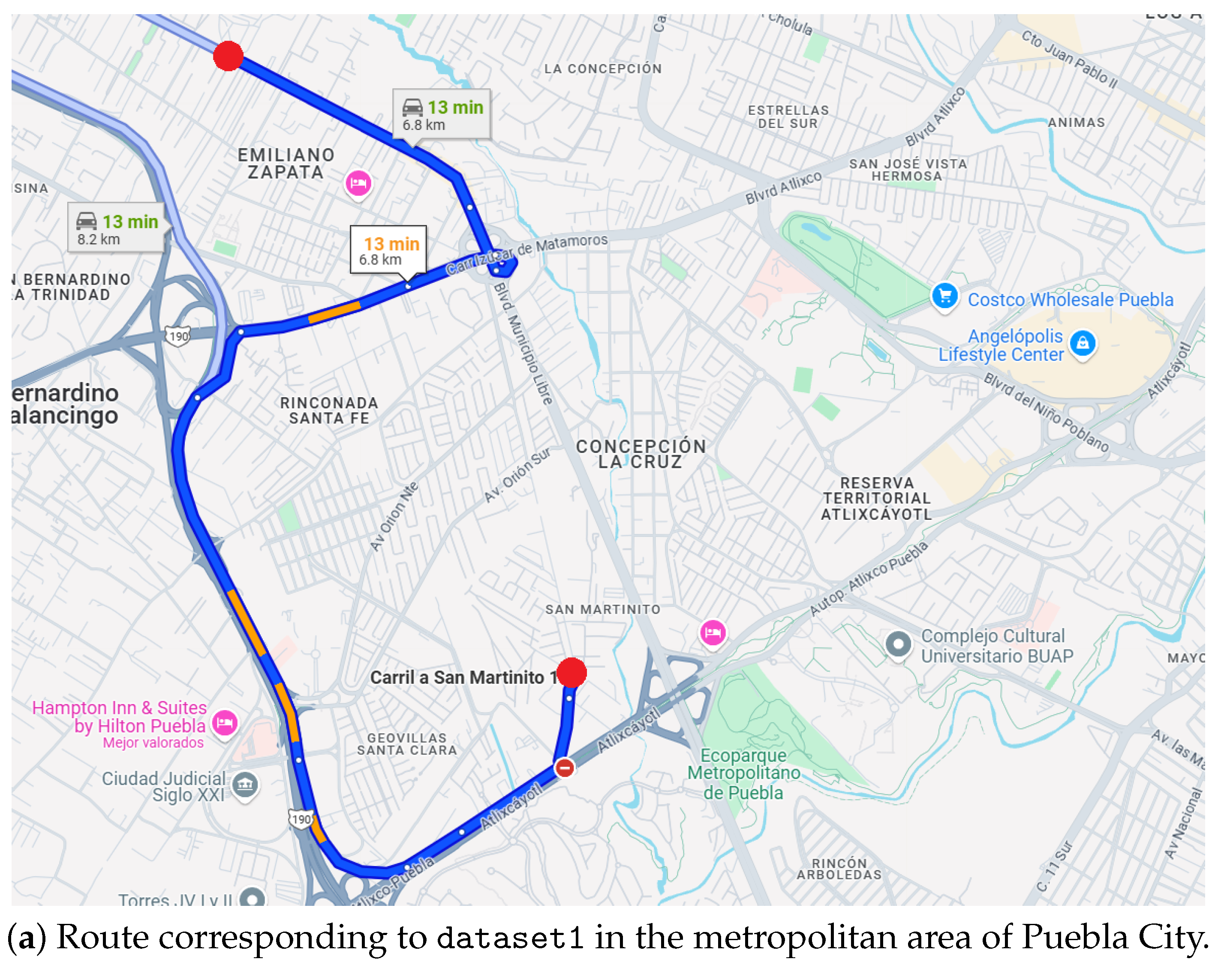
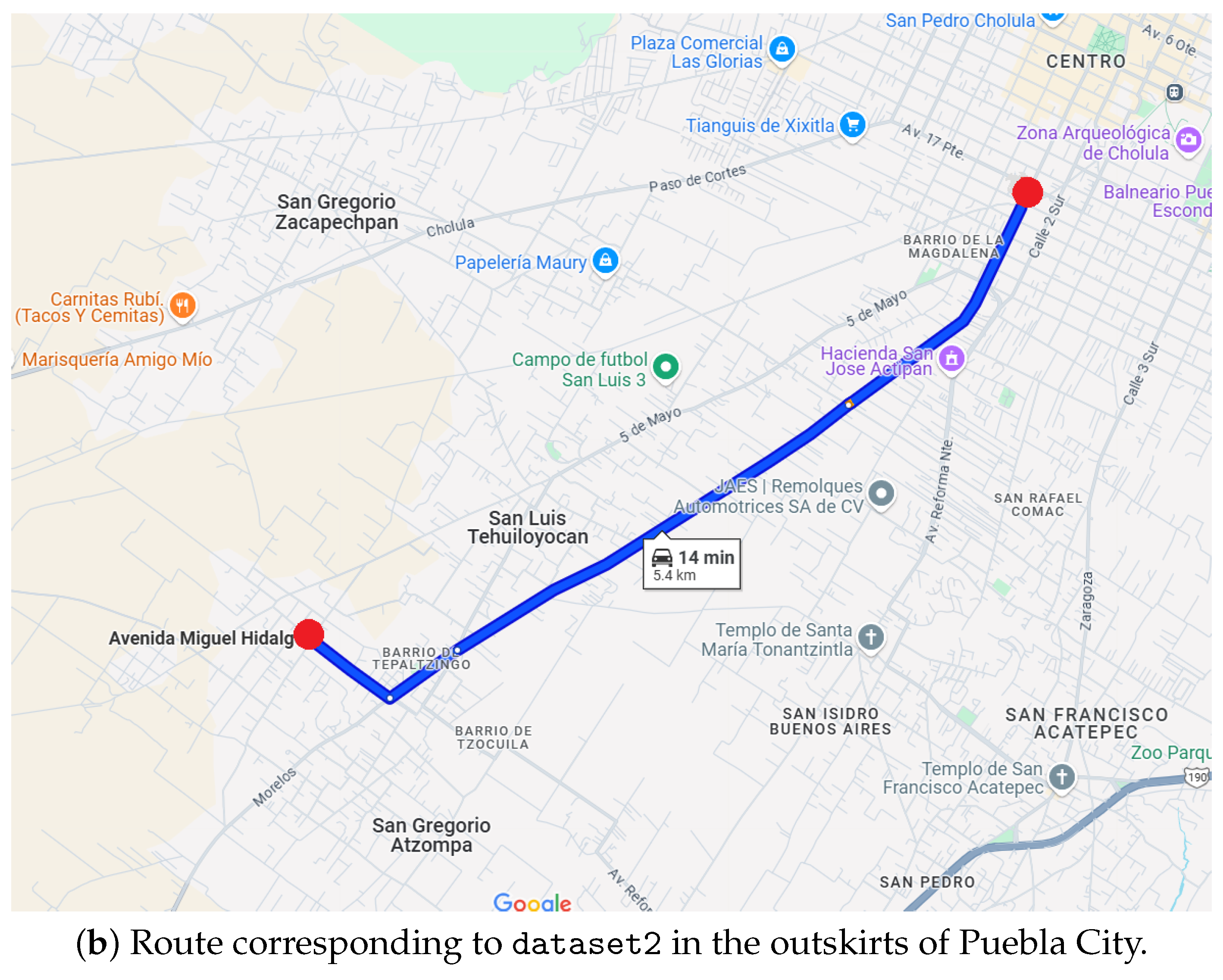
5. Dataset Description

The dataset used in this study was collected using an instrumented vehicle, which traveled along two distinct routes in San Andrés Cholula, Puebla, Mexico. These routes were specifically chosen to capture the variability in road conditions, traffic density, and urban infrastructure.

The data collection process was designed to ensure high-quality recordings, minimizing external interference. The vehicle was equipped with an AQ-1 OBDII Data Logger, a high-precision data acquisition device capable of capturing real-time vehicle dynamics. This device recorded triaxial acceleration and vibration data, securely mounted to minimize external disturbances. The sensor operated at a sampling rate of up to 1000 hz per channel, capturing high-frequency signals to detect subtle road anomalies. Data recording was carried out under controlled conditions to prevent variations due to misalignment of the sensor or environmental factors.

The data were recorded in JSON format and include the following attributes:

• Geographic coordinates: longitude and latitude.
• Vibration data: measurements along the X, Y, and Z axes (vibration_x, vibration_y, vibration_z).
• Acceleration data: measurements along the X, Y, and Z axes (acceleration_x, acceleration_y, acceleration_z).
• Event description: Labels indicating the type of event detected, including the following categories: “No events detected”, “Speed bump detected”, “Sudden braking detected”, and “pothole detected”.

The first dataset, dataset1, represents a 6.8 km trajectory that was carried out within the metropolitan area of Puebla City, Mexico. This urban route includes various types of roads, traffic conditions, and infrastructure elements such as speed bumps, intersections, and pedestrian crossings. The second dataset, dataset2, covers a 5.4 km trajectory on the outskirts of Puebla City, characterized by urban road conditions. This route provides complementary scenarios, including unpaved roads and lesser traffic density, allowing for a broader spectrum of event detection challenges.

To ensure event reliability, the labeling process combined automatic detection thresholds and manual validation. Sudden braking events were identified when the deceleration exceeded a predefined threshold of m/s². Speed bumps and potholes were annotated on the basis of road surveys and validated using field inspections. The final dataset was reviewed to ensure consistency and minimize misclassifications.

To visualize the covered routes, Figure 2 shows the trajectories recorded by the vehicle during data collection.

Both datasets are provided as supplemental files attached to this manuscript to support reproducibility and allow further research by the community. These supplementary files include labeled JSON data. The collection of these datasets ensures diversity in the recorded events and scenarios, which is crucial to train and evaluate classification algorithms under various conditions.

For all experiments, we tested our algorithm on an MSI Raider GE76 12U laptop equipped with an Intel Core i7-12700H CPU. All experiments were performed in MATLAB 2022a, providing a stable and efficient platform for model training and evaluation. The configuration of the system allowed us to handle large datasets efficiently and perform extensive hyperparameter tuning, ensuring that the Random Forest model could be trained and tested in a reasonable amount of time.

Quantitative Analysis

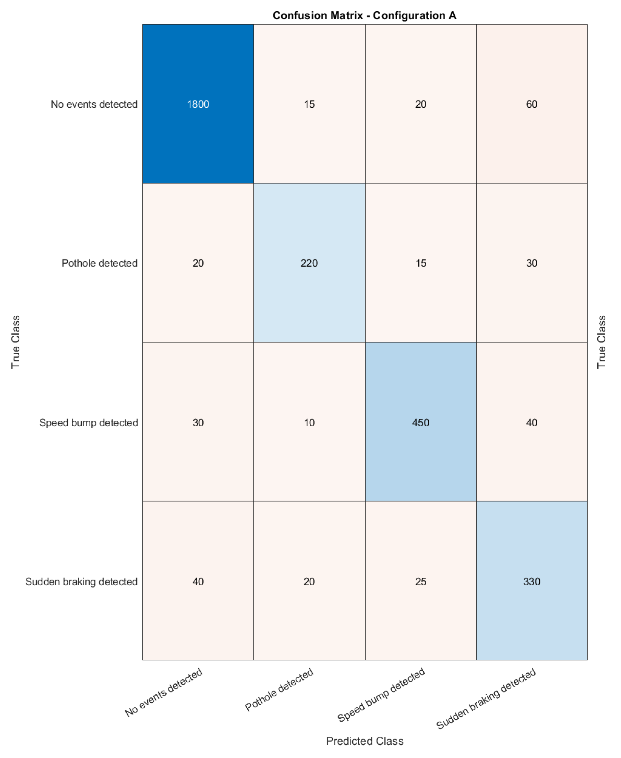
In this section, we present the results of three different configurations tested in the context of event detection and classification based on vibration and acceleration data. Each configuration is designed to optimize specific aspects of the model’s performance, such as precision, recall, and AUC (Area Under the Curve of the Receiver Operating Characteristic—ROC Curve), while addressing the challenges of class imbalance and generalization. The dataset was divided into two parts for training and testing purposes. Dataset1 was split in half, with one part used for training and the other for testing. Similarly, for Dataset2, the data were divided into two sets with the same approach. This ensured that the model was trained on one subset of the data and tested on the other, allowing for a fair evaluation of its performance. The three configurations tested are as follows:

• Configuration A: Baseline Model
  In this configuration, the Random Forest classifier was trained using the default hyperparameters to establish a baseline model. Specifically, the model used trees $N_T=100$ with default values for the maximum depth ($\max \_\mathrm{depth}=\mathrm{None}$) and the minimum samples required to split a node ($\min \_\mathrm{samples}\_\mathrm{split}=2$). The dataset was divided into training and test sets with a ratio of 50%–50% and no adjustments were made for the imbalance of the classes. The performance of the model on all class events was evaluated using standard metrics of precision, recall, and AUC (Area Under the Receiver Operating Characteristic Curve). This configuration serves as a reference for comparing more advanced configurations.
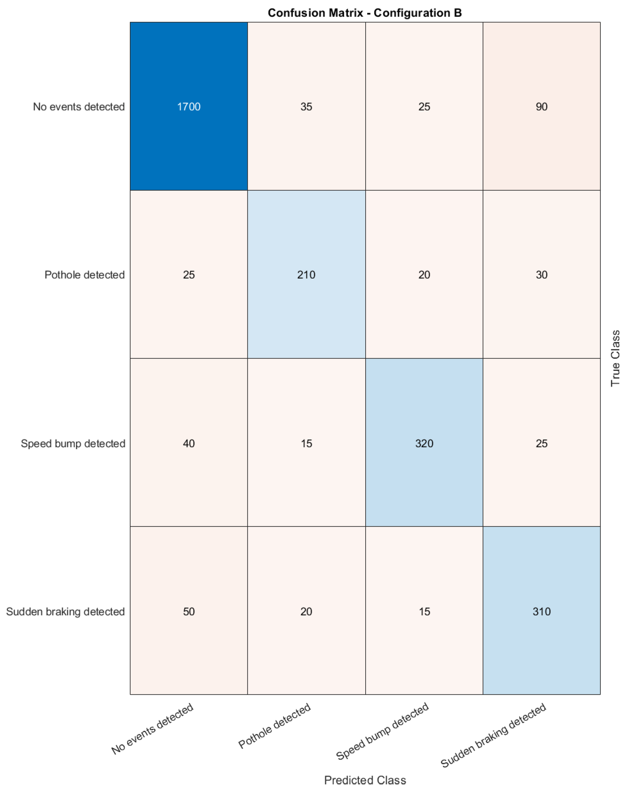
• Configuration B: Class Balanced Model
  This configuration addresses the class imbalance problem by applying class weighting during the training process. Given that the “No events detected” class is significantly overrepresented, this configuration assigns higher class weights to minority classes to ensure that the model gives adequate attention to them. The class weights are computed as the inverse of the class frequencies and are incorporated into the training of each decision tree. In addition, the dataset was split into training and testing sets using stratified k-fold cross-validation to ensure that each fold contains a proportionate representation of each class. The hyperparameters for the model remained unchanged, except for the adjustment in class weights. The Random Forest model still used trees $N_T=100$, with no constraints on tree depth or leaf samples. Performance metrics are calculated after the model is evaluated in the testing set.
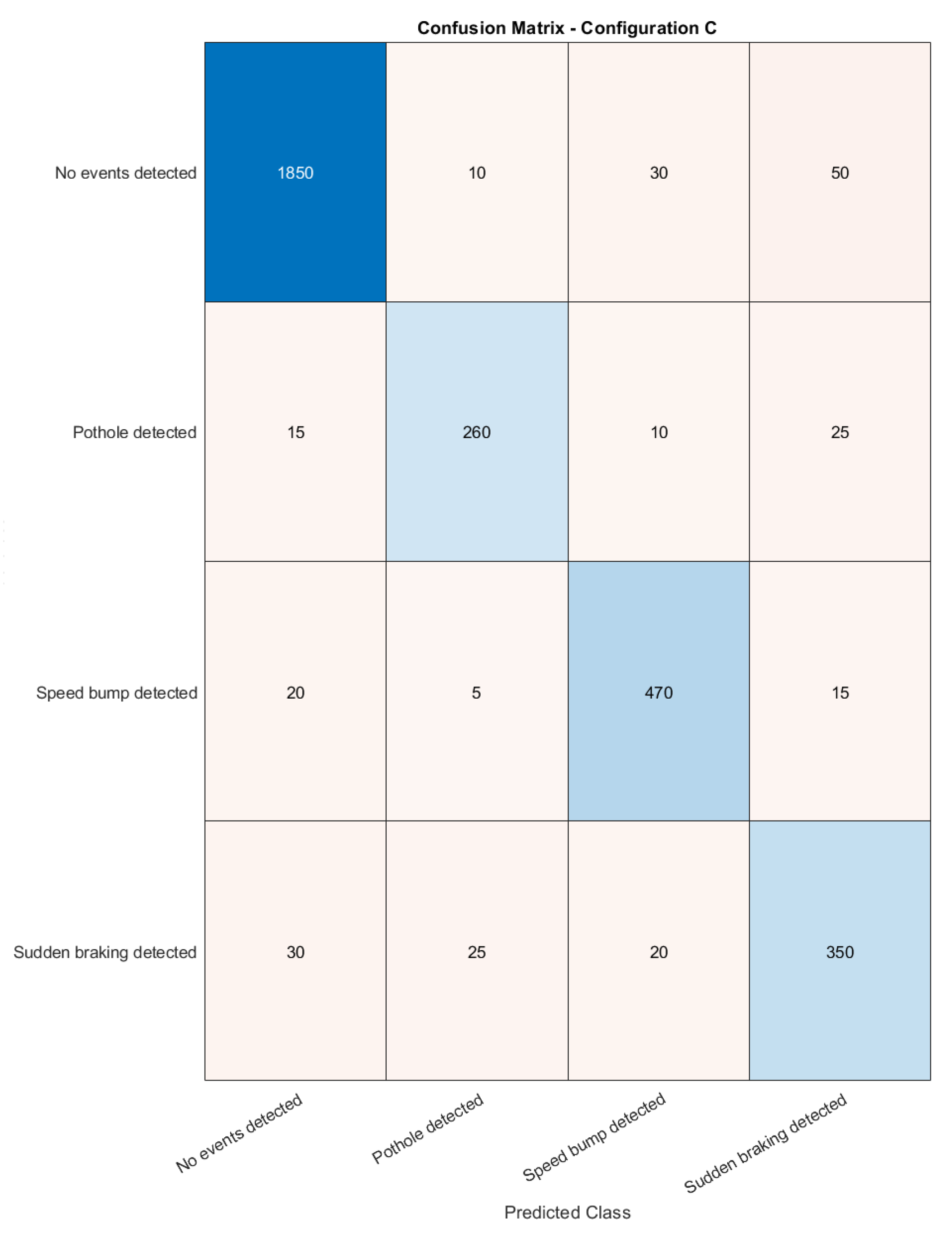
• Configuration C: Hyperparameter Tuning Model
  Configuration C represents an optimized version of the Random Forest model, where the hyperparameters are fine-tuned to achieve the best performance. The number of trees, $N_T$, varied from 100 to 200, and the maximum depth of the trees was restricted between 10 and 20 to prevent overfitting. The minimum number of samples required to split a node was varied between 2 and 10. A grid search approach was used to identify the optimal combination of these hyperparameters, and the best model was selected based on cross-validation results using a five-fold split. Additionally, class balancing was incorporated as in Configuration B, where class weights were adjusted based on the inverse of the class frequencies. Cross-validation was performed on the entire dataset, ensuring that the model’s performance generalizes well across different splits. Finally, the performance of the model was evaluated in the testing set using precision, recall, F1 score, and AUC (Area Under the Operating Characteristic Curve of the Receiver).

The results of these configurations, as shown in

Table 1. Performance comparison between the rule-based approach and Random Forest configurations A, B, and C, both with and without the Butterworth filter. Filtering consistently improves accuracy, recall, and AUC by reducing sensor noise.

Approach	Precision	Recall	F1-Score	Accuracy	AUC
Rule-Based	0.92	0.78	0.84	0.910	N/A
Random Forest (A)—No Filter	0.78	0.72	0.75	0.851	0.924
Random Forest (A)—Filtered	0.85	0.80	0.82	0.896	0.981
Random Forest (B)—No Filter	0.70	0.65	0.67	0.812	0.878
Random Forest (B)—Filtered	0.75	0.70	0.72	0.866	0.913
Random Forest (C)—No Filter	0.74	0.69	0.71	0.841	0.905
Random Forest (C)—Filtered	0.80	0.75	0.77	0.919	0.946

, provide insight into the trade-offs between precision, recall, and overall classification performance. Each configuration was evaluated based on the following metrics:

-

** Precision: ** Measures the accuracy of positive predictions.

-

** Recall: ** Assesses the ability of the model to correctly identify all relevant instances of each event.

-

** F1-Score: ** The harmonic mean of precision and recall, providing a balance between the two.

-

** Accuracy: ** The overall accuracy of the model.

-

** AUC (Area Under the Curve): ** Provides a measure of the model’s ability to discriminate between classes.

The results are summarized below in Table 1, showing performance metrics for the three configurations.

The results of the different configurations show the following key insights:

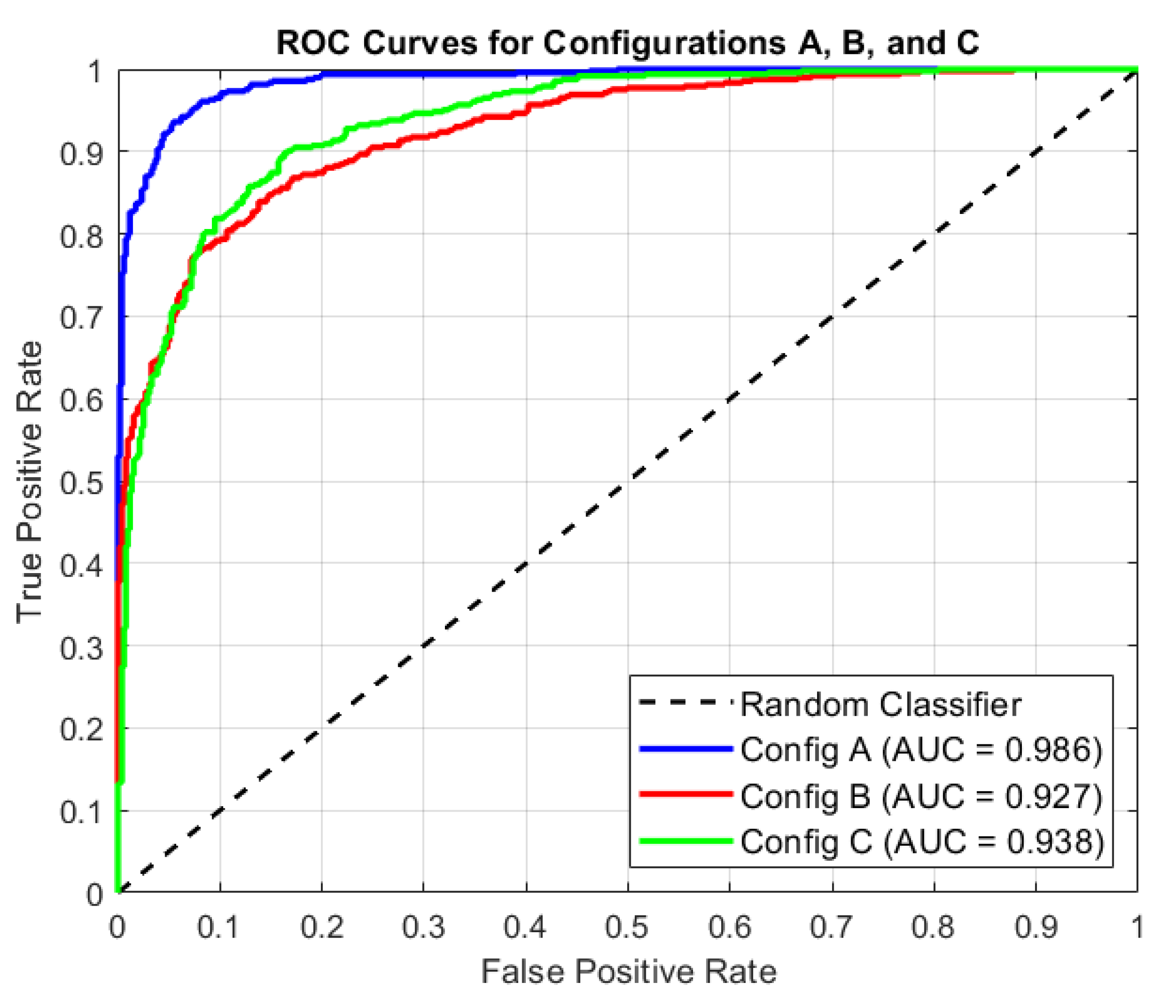
• Configuration A achieved the highest AUC value (0.98106), indicating excellent general model discrimination between event types. However, while precision and recall were balanced, there was no clear optimization for specific event classes. The model performed well in detecting both event and non-event classes but was not specifically tuned for rare event detection.
• Configuration B, incorporating class balancing adjustments, improved recall (0.75) for the “No events detected” class, which is the dominant class in the dataset. However, this came at the expense of AUC (0.91358), reflecting a trade-off in the ability to distinguish between event and nonevent classes. This adjustment was beneficial for better detecting the non-event class, but may have caused slight underperformance in event detection.
• Configuration C provided the best overall balance of precision (0.80) and recall (0.75), while also improving the AUC to 0.94682. This configuration demonstrated the effectiveness of hyperparameter tuning, balance of model complexity, and generalization. It showed the highest overall robustness and is considered the most reliable configuration for event detection, as it optimized the model for both types of events and non-events.
• Comparison with Alternative Approaches. To further evaluate the performance of our proposed method, we compared it with a rule-based approach. The rule-based model, which was primarily used for event labeling, relies on predefined thresholds for vibration and acceleration patterns. Although this approach achieves a high precision of 0.92 and accuracy of 0.910 (see Table 1), these results are **highly dependent on the adjustment of the manual parameters**.
  A fundamental limitation of the rule-based approach is its lack of generalization. For each dataset and even for different segments of the trajectory within the same dataset**, continuous manual adjustments** are required to maintain its precision. This makes the approach impractical for real-time deployment in large-scale dynamic environments, where road conditions, vehicle types, and sensor variations can significantly affect detection performance.
  Additionally, the rule-based approach does not produce a **probabilistic output**, meaning it cannot compute an AUC score. Unlike machine learning models, which can adapt to unseen data distributions, the rule-based model strictly follows predefined conditions, making it highly sensitive to variations in road events.
  In contrast, our proposed Random Forest-based approach provides a more **scalable and adaptive** solution. As shown in Table 1, despite a slight trade-off in precision, Configurations A, B, and C of the Random Forest model demonstrate **higher robustness and consistency between different datasets**. The ability to learn complex patterns from sensor data without requiring continuous manual tuning makes this approach **better suited for real-world deployment in urban traffic environments**.

The experimental results demonstrated the importance of configuration choices and how the balance between model complexity, class imbalance, and fine-tuning can affect overall performance. Configuration C, with hyperparameter adjustments and optimal balance, provides the most reliable results for event detection in the context of road event detection in urban traffic.

The results of these experiments align with the goals outlined in Section 3.3, where our aim was to build a robust and generalizable Random Forest model. Configuration A served as the baseline, while Configurations B and C addressed specific challenges such as class imbalance and the need for finer control over model parameters.

The **AUC** results show that Configuration A had the highest discriminative ability (0.98106), suggesting that the baseline model could distinguish well between the event types. However, this configuration might not have optimized the model’s ability to detect less frequent events because of the class imbalance. The **AUC** in Configuration B dropped to 0.91358, which reflects the trade-off introduced by class balancing techniques. Although recall for the “No events detected” class increased to 0.75, this led to a decrease in the ability to distinguish between event and non-event classes. On the other hand, Configuration C, with hyperparameter tuning, managed to maintain a high level of discrimination (AUC of 0.94682), along with improvements in both precision and recall, making it the most balanced configuration.

To better visualize these results, we include the following figures:

• Confusion Matrices (Figure 3, Figure 4 and Figure 5) display the confusion matrices for Configurations A, B and C, respectively, highlighting true positives, false positives, false negatives, and true negatives.
• ROC Curves (Figure 6) show the ROC curves and corresponding AUC values for Configurations A, B and C to demonstrate trade-offs between sensitivity and specificity.
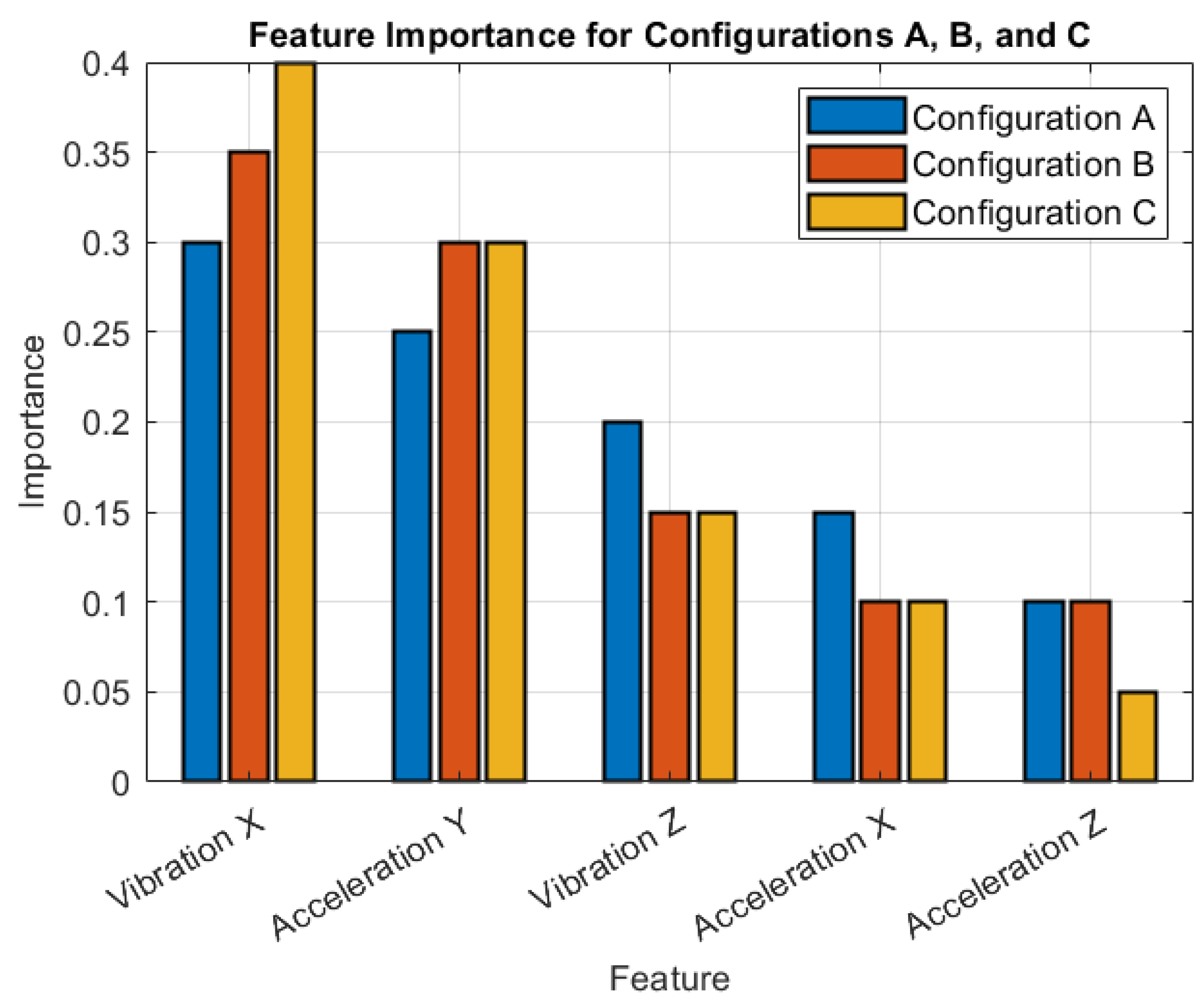
• Feature Importance (Figure 7) provides a graphical representation of the most important features identified by the Random Forest model, which are crucial for accurate event detection.

As shown in these figures, the model in Configuration C not only achieved better overall performance, but also demonstrated better ranking of importance of features, allowing the model to focus on the most relevant features for accurate classification.

These findings demonstrate that hyperparameter tuning, class balancing, and a careful balance between model complexity and interpretability are essential to improve performance in the context of road event detection.

6. Impact of the Butterworth Filter on Classification Performance

To assess the impact of signal preprocessing, we compare the classification results with and without applying a Butterworth filter to the vibration and acceleration data. As shown in Table 1, filtering ** consistently improves the performance of the model in all configurations**.

Without filtering, the classifier struggled with increased noise in raw sensor data, leading to lower accuracy and AUC scores. For example, in Configuration A, the accuracy drops from **89.6% (filtered) to 85.1% (unfiltered)**, while the AUC decreases from **0.981 to 0.924**. This trend is consistent across Configurations B and C, reinforcing the role of filtering in improving data quality.

The improvement in recall across all configurations indicates that filtering helps the model **better capture true positive events**, reducing false negatives. This is crucial for real-time applications, where missing critical road events could affect the reliability of the system.

In contrast, the rule-based approach maintains high precision but lacks adaptability across different datasets. The Random Forest model, especially with filtering, offers a more **robust and generalizable solution**, making it better suited for real-world deployment.

6.1. Algorithmic Complexity Analysis

The computational complexity of the proposed Random Forest-based event detection and classification pipeline is analyzed by breaking down its key components:

6.1.1. Data Preprocessing

• Low-Pass Filtering: Applying a Butterworth filter to vibration and acceleration data has a complexity of $O(n·m)$, where n is the number of data samples and m is the number of sensor channels (e.g., $m=3$ for the x, y, z axes). Since the filter coefficients are constant for a fixed filter order, this operation scales linearly with the number of samples.
• Normalization: Min–Max normalization involves finding the minimum and maximum values for each channel, which is $O\left(n\right)$, followed by a linear transformation of the data, also $O\left(n\right)$. The overall complexity remains $O\left(n\right)$.

6.1.2. Feature Extraction

• Sliding Window: Using a sliding window approach with a size of w and overlap o, the number of windows processed is approximately $(n-w)/(w-o)$. Extracting the features for each window involves the following:

  -

  Statistical Features (mean, variance, skewness, kurtosis): $O\left(w\right)$ each.

  -

  Frequency features (FFT, spectral entropy): FFT has a complexity of $O(wlogw)$, and the entropy calculation is $O\left(w\right)$.

  Overall Complexity: $O\left({\displaystyle \frac{n-w}{w-o}}·wlogw\right)$, dominated by the FFT computation.

6.1.3. Model Training

• Random Forest Training: The complexity of training a Random Forest model depends on the following:

  -

  T: Number of trees in the forest.

  -

  d: Maximum depth of each tree.

  -

  f: Number of features considered in each split.

  -

  m: Number of samples in the training set.

  For a single tree, the complexity is $O(m·f·d)$. For trees T, it becomes $O(T·m·f·d)$. Key Insight: Increasing T improves the performance of the model, but also increases the computational cost linearly.

6.1.4. Inference

• Prediction: During inference, the complexity of a single prediction is proportional to the number of trees T and the depth of each tree d, i.e., $O(T·d)$.
• Sliding Window for Testing: Similar to feature extraction, the prediction process for test data also uses a sliding window approach. The total complexity is $O\left({\displaystyle \frac{n-w}{w-o}}·T·d\right)$.

6.1.5. Summary of Complexity

• Preprocessing: $O(n·m)$.
• Feature Extraction: $O\left({\displaystyle \frac{n-w}{w-o}}·wlogw\right)$.
• Training: $O(T·m·f·d)$.
• Inference: $O\left({\displaystyle \frac{n-w}{w-o}}·T·d\right)$.

This analysis highlights the trade-offs between computational cost and performance in each stage of the pipeline, underscoring the need for optimization to balance accuracy and efficiency.

6.2. Real-Time Processing and Embedded System Implementation

The Random Forest model processes sensor data in real time, allowing for rapid classification of road events such as “speed bumps”, “sudden braking”, and “potholes”. The computational time of the model per feature vector is minimal, enabling the system to make predictions rapidly. We balance the accuracy and processing speed of the model by adjusting the number of trees ($N_T$) and the depth of the tree, optimizing the performance without compromising real-time requirements. The optimized Random Forest model developed in this study was designed with the potential for deployment in embedded systems, particularly for real-time event detection tasks. Several optimization techniques were applied to balance model accuracy with the processing and memory requirements typical of systems with limited resources.

• Model Pruning: The tree depth was reduced to decrease memory usage and computational load, making the model more suitable for platforms with limited processing power.
• Feature Selection: Only the most important features were used, reducing the input dimensionality and improving the processing speed without significantly affecting the model’s performance.
• Quantization and Optimization: Techniques such as weight quantization were applied to reduce memory and computational demand, improving the feasibility of deploying the model on embedded devices constrained by resources.

These optimizations contribute to reduced latency and improved efficiency, making the model suitable for real-time applications such as vehicle event detection systems. In conclusion, the optimized Random Forest model provides a good balance of performance, speed, and efficiency, allowing for deployment in embedded systems without the need for specialized hardware.

7. Current Scope and Limitations

The proposed approach, based on a Random Forest classifier, offers a robust and efficient solution for real-time road event detection using vibration and acceleration data. Our method leverages multiaxis sensor data (x, y, z) to enhance classification accuracy, distinguishing itself from traditional single-axis or rule-based techniques. By incorporating dynamic feature extraction and noise reduction, the algorithm provides improved adaptability to various urban traffic conditions. Furthermore, unlike deep learning-based methods, which often require extensive labeled datasets and high computational resources, our approach maintains high classification accuracy with lower computational overhead [23].

However, certain limitations must be acknowledged. First, while the Random Forest model effectively handles various road events, its performance can be impacted by variations in road conditions in different geographical regions. Training the model on a more extensive and diverse dataset could further improve generalization [24]. Second, the current implementation does not integrate additional sensor modalities, such as gyroscopes or GPS, which could improve classification accuracy in ambiguous scenarios. Finally, while the model is optimized for real-time processing suitable for resource-constrained embedded systems, it may require further optimizations, such as model pruning or feature selection [25].

To address these limitations, future work will focus on expanding the dataset to include more diverse driving environments, integrating multi-modal sensor data, and optimizing the algorithm for low-power embedded systems. In addition, exploring deep learning architectures or hybrid models could further improve event classification performance while maintaining computational efficiency [26].

Future Work

Although the proposed random forest-based event detection and classification approach demonstrates promising results, there are several areas for future research and improvement:

• Integration with Real-Time Systems: Extending the current offline analysis to a real-time system capable of processing vibration and acceleration data on embedded hardware. This involves optimizing the computational pipeline to meet the constraints of latency and power consumption.
• Advanced Machine Learning Models: Exploring advanced machine learning techniques, such as deep learning models, to capture more complex patterns in the data. Recurrent Neural Networks (RNNs) or Convolutional Neural Networks (CNNs) could be particularly effective in identifying spatio-temporal dependencies.
• Extended Event Categories: Expanding the scope of event detection to include additional road event detection, such as lane changes, overtaking, and sharp turns, to enhance the utility of the model in multiple environments.
• Multimodal Data Fusion: Incorporating additional sensors, such as GPS, gyroscopes, or cameras, to create a multimodal system. This would improve the accuracy of the classification and provide a richer context for detected events.
• Generalization Across Locations: Testing and adapting the model for different geographical regions to ensure robustness against variations in road conditions, vehicle types, and driving behaviors.
• Explainability and Interpretability: Develop methods to improve the interpretability of the model’s decisions, particularly in scenarios where safety-critical decisions are required. Feature attribution techniques and visualization tools could provide valuable insights into model behavior.
• Scalability for Large Datasets: Investigating scalable training techniques to handle larger datasets with higher-dimensional feature spaces, ensuring that the model remains efficient and applicable to industrial-scale deployments.

These directions aim to address both technical challenges and practical considerations, paving the way for a more comprehensive and deployable solution for road event detection in urban traffic.

8. Conclusions

This work presents a Random Forest-based approach for event detection and classification in road event detection, using vibration and acceleration data. The results demonstrate the effectiveness of the proposed method in detecting events such as speed bumps, sudden braking, and potholes, while addressing challenges such as class imbalance and feature variability.

Key findings of this research include the following.

• The baseline model (Configuration A) provided a solid foundation, achieving an AUC of 0.98106. However, it exhibited limitations in optimizing precision and recall for minority classes.
• Configuration B demonstrated the importance of addressing the class imbalance by improving recall for the majority class, although it came at the cost of slightly reduced overall accuracy and AUC.
• Configuration C, which incorporated hyperparameter tuning, achieved the best balance between precision (0.80), recall (0.75), and AUC (0.94682), demonstrating its robustness for real-world applications.

Analysis of algorithmic complexity revealed that the computational demands of feature extraction and model training remain feasible for offline implementations but may require optimization for real-time applications. Furthermore, the results highlighted the importance of feature engineering and parameter tuning in improving model performance.

This research contributes to the field of road event detection by providing a scalable and interpretable framework for event detection using accessible sensor data. The proposed methodology is versatile and can be adapted to other domains that involve similar data types.

References

1. Rathee, M.; Bačić, B.; Doborjeh, M. Automated road defect and anomaly detection for traffic safety: A systematic review. Sensors 2023, 23, 5656. [Google Scholar] [CrossRef] [PubMed]
2. Kyriakou, C.; Christodoulou, S.E.; Dimitriou, L. Do vehicles sense, detect and locate speed bumps? Transp. Res. Procedia 2021, 52, 203–210. [Google Scholar] [CrossRef]
3. Misra, M.; Mani, P.; Tiwari, S. Early Detection of Road Abnormalities to Ensure Road Safety Using Mobile Sensors. In Ambient Communications and Computer Systems: Proceedings of RACCCS 2021; Springer: Berlin/Heidelberg, Germany, 2022; pp. 69–78. [Google Scholar]
4. Bala, J.A.; Adeshina, S.A.; Aibinu, A.M. Advances in Road Feature Detection and Vehicle Control Schemes: A Review. In Proceedings of the IEEE 2021 1st International Conference on Multidisciplinary Engineering and Applied Science (ICMEAS), Abuja, Nigeria, 15–16 July 2021; pp. 1–6. [Google Scholar]
5. Ozoglu, F.; Gökgöz, T. Detection of road potholes by applying convolutional neural network method based on road vibration data. Sensors 2023, 23, 9023. [Google Scholar] [CrossRef] [PubMed]
6. Celaya-Padilla, J.M.; Galván-Tejada, C.E.; López-Monteagudo, F.E.; Alonso-González, O.; Moreno-Báez, A.; Martínez-Torteya, A.; Galván-Tejada, J.I.; Arceo-Olague, J.G.; Luna-García, H.; Gamboa-Rosales, H. Speed bump detection using accelerometric features: A genetic algorithm approach. Sensors 2018, 18, 443. [Google Scholar] [CrossRef] [PubMed]
7. Dogru, N.; Subasi, A. Traffic accident detection using random forest classifier. In Proceedings of the IEEE 2018 15th Learning and Technology Conference (L&T), Jeddah, Saudi Arabia, 25–26 February 2018; pp. 40–45. [Google Scholar]
8. Su, Z.; Liu, Q.; Zhao, C.; Sun, F. A traffic event detection method based on random forest and permutation importance. Mathematics 2022, 10, 873. [Google Scholar] [CrossRef]
9. Jiang, H.; Deng, H. Traffic incident detection method based on factor analysis and weighted random forest. IEEE Access 2020, 8, 168394–168404. [Google Scholar] [CrossRef]
10. Rigatti, S.J. Random forest. J. Insur. Med. 2017, 47, 31–39. [Google Scholar] [CrossRef] [PubMed]
11. Biau, G.; Scornet, E. A random forest guided tour. Test 2016, 25, 197–227. [Google Scholar] [CrossRef]
12. Parmar, A.; Katariya, R.; Patel, V. A review on random forest: An ensemble classifier. In Proceedings of the International Conference on Intelligent Data Communication Technologies and Internet of Things (ICICI) 2018, Coimbatore, India, 7–8 August 2018; Springer: Berlin/Heidelberg, Germany, 2019; pp. 758–763. [Google Scholar]
13. Behera, B.; Sikka, R. Deep learning for observation of road surfaces and identification of path holes. Mater. Today Proc. 2023, 81, 310–313. [Google Scholar] [CrossRef]
14. Peralta-López, J.E.; Morales-Viscaya, J.A.; Lázaro-Mata, D.; Villaseñor-Aguilar, M.J.; Prado-Olivarez, J.; Pérez-Pinal, F.J.; Padilla-Medina, J.A.; Martínez-Nolasco, J.J.; Barranco-Gutiérrez, A.I. Speed bump and pothole detection using deep neural network with images captured through zed camera. Appl. Sci. 2023, 13, 8349. [Google Scholar] [CrossRef]
15. Martinelli, A.; Meocci, M.; Dolfi, M.; Branzi, V.; Morosi, S.; Argenti, F.; Berzi, L.; Consumi, T. Road surface anomaly assessment using low-cost accelerometers: A machine learning approach. Sensors 2022, 22, 3788. [Google Scholar] [CrossRef] [PubMed]
16. Karim, A.; Adeli, H. Incident detection algorithm using wavelet energy representation of traffic patterns. J. Transp. Eng. 2002, 128, 232–242. [Google Scholar] [CrossRef]
17. Martikainen, J.P. Learning the Road Conditions. Ph.D. Thesis, University of Helsinki, Helsinki, Finland, 2019. [Google Scholar]
18. Salman, A.; Mian, A.N. Deep learning based speed bumps detection and characterization using smartphone sensors. Pervasive Mob. Comput. 2023, 92, 101805. [Google Scholar] [CrossRef]
19. Kempaiah, B.U.; Mampilli, R.J.; Goutham, K. A Deep Learning Approach for Speed Bump and Pothole Detection Using Sensor Data. In Emerging Research in Computing, Information, Communication and Applications: ERCICA 2020; Springer: Berlin/Heidelberg, Germany, 2022; Volume 1, pp. 73–85. [Google Scholar]
20. Kim, G.; Kim, S. A road defect detection system using smartphones. Sensors 2024, 24, 2099. [Google Scholar] [CrossRef] [PubMed]
21. Menegazzo, J.; von Wangenheim, A. Speed Bump Detection Through Inertial Sensors and Deep Learning in a Multi-contextual Analysis. SN Comput. Sci. 2022, 4, 18. [Google Scholar] [CrossRef]
22. Kumar, T.; Acharya, D.; Lohani, D. A Data Augmentation-based Road Surface Classification System using Mobile Sensing. In Proceedings of the IEEE 2023 International Conference on Computer, Electronics & Electrical Engineering & their Applications (IC2E3), Srinagar Garhwal, India, 8–9 June 2023; pp. 1–6. [Google Scholar]
23. Abu Tami, M.; Ashqar, H.I.; Elhenawy, M.; Glaser, S.; Rakotonirainy, A. Using multimodal large language models (MLLMs) for automated detection of traffic safety-critical events. Vehicles 2024, 6, 1571–1590. [Google Scholar] [CrossRef]
24. Chen, B.; Fang, M.; Wei, H. Incorporating prior knowledge for domain generalization traffic flow anomaly detection. Neural Comput. Appl. 2024, 1–14. [Google Scholar] [CrossRef]
25. Radak, J.; Ducourthial, B.; Cherfaoui, V.; Bonnet, S. Detecting road events using distributed data fusion: Experimental evaluation for the icy roads case. IEEE Trans. Intell. Transp. Syst. 2015, 17, 184–194. [Google Scholar] [CrossRef]
26. Khan, Z.; Tine, J.M.; Khan, S.M.; Majumdar, R.; Comert, A.T.; Rice, D.; Comert, G.; Michalaka, D.; Mwakalonge, J.; Chowdhury, M. Hybrid quantum-classical neural network for incident detection. In Proceedings of the IEEE 2023 26th International Conference on Information Fusion (FUSION), Charleston, SC, USA, 27–30 June 2023; pp. 1–8. [Google Scholar]
Figure 1. Block diagram of the proposed event classification algorithm. The pipeline consists of four main stages: (1) Data Preprocessing, where raw vibration and acceleration signals from the x, y, and z axes are collected, filtered, and normalized; (2) Feature Extraction, which derives statistical and frequency-based characteristics from sensor data; (3) Model Training, where a Random Forest classifier is built using extracted features; and (4) Event Classification, in which the trained model categorizes incoming sensor data into predefined event types.
Algorithms 18 00127 g001
Figure 2. Visualization of the trajectories recorded for data collection. The urban route (a) covers 6.8 km within the metropolitan area of Puebla City, while the suburban route (b) covers 5.4 km on the outskirts of the city.
Algorithms 18 00127 g002aAlgorithms 18 00127 g002b
Figure 3. Confusion matrix for Configuration A.
Algorithms 18 00127 g003
Figure 4. Confusion matrix for Configuration B.
Algorithms 18 00127 g004
Figure 5. Confusion matrix for Configuration C.
Algorithms 18 00127 g005
Figure 6. Combined ROC curves for Configurations A, B, and C. The figure compares the performance of each configuration, where Configuration A (blue), Configuration B (red), and Configuration C (green) are plotted together for a fair comparison. A diagonal reference line represents a random classifier.
Algorithms 18 00127 g006
Figure 7. Feature importance comparison for Configurations A, B, and C. The bar plot illustrates the contribution of each feature (Vibration X, Acceleration Y, Vibration Z, Acceleration X, and Acceleration Z) across different configurations.
Algorithms 18 00127 g007