Abstract
Traditional heat diffusion systems are typically regulated using Proportional–Integral–Derivative (PID) controllers. PID controllers still remain the backbone of numerous industrial control applications due to their simplicity, robustness, and efficiency. However, traditional tuning methods—such as Ziegler–Nichols or Cohen–Coon—often exhibit limitations when applied to systems with nonlinear dynamics, time-varying behaviors, or parametric uncertainties. To address these challenges, Fuzzy Logic Controllers (FLC) have emerged as a promising hybrid strategy, by translating quantitative and imprecise linguistic inputs into quantitative control actions, thereby enabling more adaptive and precise regulation. This is achieved through the integration of fuzzy inference mechanisms that dynamically adjust PID gains in response to changing system conditions. This study proposes a fuzzy logic control strategy for a heat diffusion system and conducts a comparative analysis against conventional PID control. The methodology encompasses system modeling, design of the fuzzy inference system, and simulation studies. To improve transient response and address time delays, additional features such as Anti-Windup compensation and a Smith Predictor are integrated into the control scheme. The final validation step involves the introduction of simulated environmental disturbances, including abrupt temperature drops, to evaluate the controller’s robustness. Simulation results demonstrate that the proposed FLC provides superior dynamic performance compared to the conventional PID controller, achieving approximately 5–7% faster rise time and 8–10% lower settling time. The incorporation of an anti-windup mechanism did not yield significant benefits in this application. In contrast, the integration of a Smith Predictor further reduced oscillatory behavior and substantially improved disturbance rejection, tracking accuracy, and adaptability under simulated thermal variations. These results underscore the effectiveness of the FLC in handling systems with time delays and nonlinearities, reinforcing its role as a robust and adaptable control strategy for thermal processes with complex dynamics.
1. Introduction
Automatic control systems play a crucial role in modern applications ranging from complex industrial processes to building HVAC, and thermal management in electronic devices and thermal process control. However, the control of thermal systems presents significant challenges [1]. Heating and cooling systems operate in dynamic environments subject to external disturbances, such as the opening of doors and windows, which cause abrupt temperature variations. Additionally, heat diffusion processes inherently involve propagation delays and nonlinear behaviors, complicating precise regulation using conventional control methodologies [2,3,4,5].
Several real-world systems exhibiting such time delays have been extensively studied:
- Building HVAC systems, where the thermal inertia of walls and air results in slow and delayed responses to control inputs [6];
- Industrial furnaces and heat exchangers, where delays are accentuated due to material transport times and thermal conduction lags [7,8,9];
- Chemical processing plants, where time delays arise from reagent mixing times and the propagation of temperature and pressure changes through reactors [10].
Although PID controllers remain the dominant control strategy in industry, they exhibit limitations in dynamic environments [11,12]. Their reliance on linear models and fixed parameters reduces effectiveness when confronted with disturbances and parameter variations. In this context, alternative approaches such as Fuzzy Logic gain importance. Drawing inspiration from human reasoning under uncertainty, fuzzy logic enables the translation of qualitative rules (e.g., “If the temperature is low, increase heating”) into quantitative control actions, thereby enhancing adaptability in complex and unpredictable systems [13].
This paper aims to advance the understanding of PID and FLCs controllers, focusing on their applicability to systems with time delays. To this end, an innovative control strategy is proposed, integrating model-based compensation with intelligent control techniques. The methodology is implemented and evaluated on a delayed thermal diffusion system modeled as a first-order plus time delay (FOPTD) process.
While traditional studies often address FLCs, anti-windup mechanisms, and the Smith Predictor as independent control solutions, this work distinguishes itself by proposing a unified control architecture that synthesizes these strategies to leverage their complementary strengths.
The primary contribution of this study lies in the development and assessment of a hybrid control framework that combines the predictive accuracy of model-based compensation with the adaptive, nonlinear handling capabilities of fuzzy logic control. This integration enables enhanced dynamic response, improved stability margins, and increased robustness in the presence of time delays and model uncertainties—challenges frequently encountered in thermal systems and other industrial processes.
To validate the proposed approach, a comprehensive set of control schemes—including conventional PID and Fuzzy-PID controllers, both with and without compensation—is designed and systematically analyzed. Controller performance is evaluated using consistent quantitative performance indices and comparative graphical analyses, ensuring a transparent and rigorous assessment of each configuration’s effectiveness.
By demonstrating the performance enhancements achieved through this hybrid methodology, the study contributes to the advancement of intelligent control system design. It offers practical insights into the development of adaptable and resilient control architectures capable of addressing the inherent limitations of traditional methods. The findings underscore the potential of integrating model-based and intelligent control techniques to realize more robust, flexible, and high-performance solutions for systems characterized by time delays and nonlinear behavior.
This paper is structured to provide a comprehensive and coherent analysis of advanced control strategies for heat diffusion systems with time delay. It begins with the Introduction, outlining the motivation, objectives, and relevance of using intelligent control techniques in thermal systems. The Heat Diffusion Systems, Section 2, introduces the physical principles and modeling considerations of the system under study. Next, Fuzzy Logic Controllers are presented in Section 3, highlighting their design, advantages, and how they differ from classical control approaches. The System Implementation section, Section 4, details the development and configuration of the control architecture, including both PID and Fuzzy-based strategies. In Section 5, Simulations and Results, various scenarios are explored to assess the controllers’ performance under ideal and perturbed conditions, with and without model-based enhancements like the Smith Predictor. A Practical Case Study follows in Section 6, testing the controllers in a more realistic environment with external disturbances. Finally, the Conclusions, Section 7, summarize the key findings, emphasizing the superior performance of the Fuzzy-PID controller combined with model-based compensation techniques. This structure ensures a logical flow from theoretical background to practical validation.
2. Heat Diffusion System
A primary objective in conduction analysis is to determine the temperature distribution within a medium based on the prescribed boundary conditions [14,15]. The temperature field in a solid is governed by the heat diffusion equation, which characterizes the spatial and temporal evolution of temperature [16,17]. For a medium with constant thermal conductivity, the governing equation in Cartesian coordinates is expressed as
where T is the temperature field, q is the volumetric heat generation rate, k is the thermal conductivity, and is the thermal diffusivity, with denoting density and the specific heat capacity of the material.
Depending on the underlying assumptions—such as steady-state conditions or the absence of internal heat generation—Equation (1) simplifies to classical forms, including the Laplace and Poisson equations [18].
Modeling Systems with Delay
Due to the inherently slow propagation of heat, thermal systems often exhibit significant time delays, or dead time , between the implementation of a control action and its measurable effect. A widely adopted simplified representation of such systems is the first-order plus time delay (FOPTD) model [14,15]:
where K is the system gain, is the time constant, and is the time delay.
In thermal applications, the time delay may arise from factors such as sensor placement, heat propagation through conduction paths, or actuator response latency. The time constant characterizes the system’s thermal inertia, governing the rate at which temperature changes in response to energy input, while the gain K quantifies the steady-state temperature variation resulting from a input.
The FOPTD model is particularly well-suited for control design, as it provides an effective compromise between simplicity and accuracy of the slow thermal dynamics, making it applicable to a broad range of practical thermal systems. It captures the dominant dynamics by representing the system as a first-order linear process with a time constant and steady-state gain, in combination with a pure time delay [14,15,19,20].
Although the FOPTD model neglects spatial temperature gradients and higher-order nonlinearities, these simplifications were compensated by using adaptive control strategies such as Fuzzy Logic and advanced techniques like the Smith Predictor and Anti-Windup, which enhance robustness against model inaccuracies and delays. This model offers a practical and computationally efficient approximation, bridging the gap between the underlying physical processes described by the heat diffusion equation and the control strategies commonly implemented in engineering applications.
3. Fuzzy Logic Controllers
Fuzzy Logic Controllers (FLCs) are intelligent control systems designed to manage uncertainty and imprecision through the use of linguistic rules and fuzzy sets [21]. Unlike traditional controllers such as PID, which depend on precise mathematical models, FLCs excel in nonlinear and time-varying environments.
An FLC typically consists of four main components:
- Fuzzification: transforms crisp input variables into fuzzy sets;
- Rule Base: a collection of IF-THEN linguistic rules representing expert knowledge;
- Inference Mechanism: applies fuzzy logic operators to evaluate the rules;
- Defuzzification: converts the fuzzy output sets into a crisp control action.
These controllers mimic human decision-making processes (e.g., “If temperature is high, then reduce heating”) and are especially advantageous in systems where precise mathematical modeling is challenging. Their effectiveness has been widely demonstrated in thermal applications, including HVAC systems, process control, and heat exchangers [22].
Fuzzy Controllers Classification
Despite the proven reliability of classical PID controllers in many applications, their fixed gain structure limits adaptability when dealing with systems characterized by nonlinearities, parametric uncertainties, or variable dynamics. To address these limitations, hybrid control strategies that integrate fuzzy logic with PID control—commonly referred to as fuzzy-PID controllers—have been developed. These controllers preserve the conventional PID framework while incorporating fuzzy logic to enhance robustness and improve control performance (Figure 1) [22].
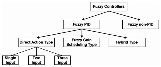
Figure 1.
Classification of fuzzy controllers [23].
Fuzzy controllers are generally categorized into two primary types: non-PID controllers, which directly generate the control signal based on fuzzy inference rules and are particularly suitable for systems that are difficult to model; and fuzzy-PID controllers, which retain the traditional PID structure but employ fuzzy logic to adapt controller parameters dynamically, thereby enhancing performance. The fuzzy-PID class can be further subdivided into three variants [24,25]:
- Direct Action: where the fuzzy controller directly computes the control signal, including fuzzy P, PI, PD, or PID configurations;
- Gain Scheduling: where fuzzy logic dynamically adjusts the PID gains , , and according to the system’s operating conditions;
- Hybrid: which integrates additional intelligent techniques, such as neural networks or genetic algorithms, and is used in complex and adaptive control applications.
The application of fuzzy control for PID tuning has been well documented in previous studies. However, this work investigates the impact of incorporating additional control structures—specifically Anti-Windup mechanisms and the Smith Predictor—into the control system. The aim is to enhance the temporal performance, particularly in terms of transient and steady-state responses.
4. System Implementation
This section outlines the theoretical framework and tools employed for modeling the heat diffusion system. It begins with a rationale for the selection of parameters characterizing the first-order time-delayed system. Subsequently, the MATLAB Fuzzy Logic Toolbox is introduced, highlighting its capabilities for designing fuzzy controllers, alongside the self-tuning features of the PID controller. Finally, the performance metrics used to assess and compare the various control strategies are presented.
4.1. System Specifications
As outlined earlier, this study aims to design and assess a controller for application in a heat diffusion system. The system under consideration consists of a planar, perfectly insulated surface, where a constant temperature boundary condition is imposed at the position m, and the resulting heat propagation is examined along the horizontal axis.
Within this configuration, a step input, defined as , is introduced at m, and the temperature response is measured at a downstream location, specifically at m.
Under these assumptions, the heat diffusion dynamics can be effectively approximated using a first-order plus time delay (FOPTD) model, as detailed in Section 2. Furthermore, the simplicity of the FOPTD structure enables systematic controller tuning through well-established methods such as the Ziegler–Nichols or Cohen-Coon approaches, facilitating real-time implementation in embedded platforms and industrial automation systems.
The system parameters were defined as , s and s, in accordance with the values proposed in [26], which have been validated in previous studies involving thermal systems with comparable characteristics, where a unit step input () was applied. The dynamic behavior of the thermal system under this step input is illustrated in Figure 2. These parameters indicate that the system exhibits slow dynamics and significant time delay, which are characteristic features of thermal processes.
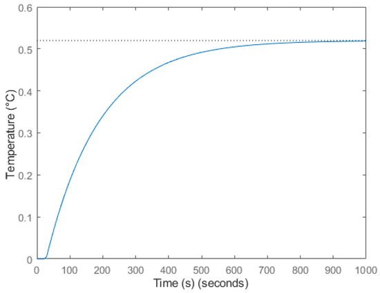
Figure 2.
Step response of the heat diffusion system, with the dashed line showing the steady-state value.
In this study, a more realistic operational scenario is considered by simulating a temperature range between 15 °C and 30 °C. This range corresponds to typical indoor thermal conditions and provides a representative context for evaluating the effectiveness of the proposed control strategies at the spatial location m along the rod.
4.2. Fuzzy Logic Toolbox
The implementation of fuzzy logic control in this work is carried out using the Fuzzy Logic Toolbox in MATLAB R2023b [27], which facilitates the development of intelligent control systems by replacing complex mathematical formulations with intuitive, rule-based logic. Upon launching the toolbox, users can select from four predefined fuzzy inference models—Mamdani Type 1, Mamdani Type 2, Sugeno Type 1, and Sugeno Type 2—or construct a fully customized system. For illustrative purposes, a Mamdani Type 1 model was adopted, representing a generic configuration with two inputs and one output, each defined by three membership functions, and governed by a rule base comprising nine rules (Figure 3).
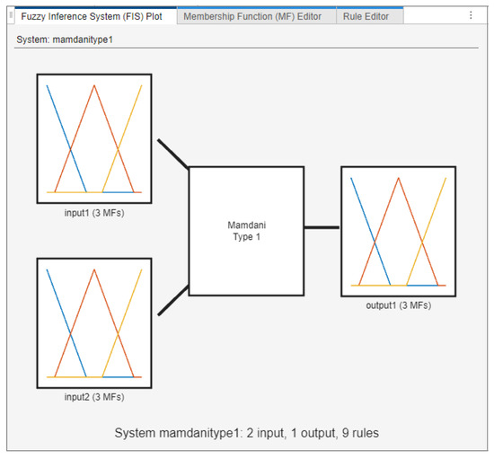
Figure 3.
General structure of the Mamdani Type 1 fuzzy controller.
The Mamdani inference model was chosen due to its superior interpretability of linguistic rules and the intuitive visualization of membership functions, which supports the goal of illustrating the design and behavior of fuzzy control systems. In contrast, the Sugeno model, although computationally efficient, is better suited for optimization-based or data-driven control applications, as it relies on mathematical functions rather than rule-based interpretability.
The Fuzzy Inference System (FIS) is fully configurable, allowing users to adjust logical operations such as AND/OR conditions, implication, aggregation methods, and the defuzzification technique. The membership functions for both input and output variables can be visualized and modified through the Membership Function Editor (Figure 4), enabling fine-tuning of the fuzzy sets to better reflect the behavior of the system under analysis.
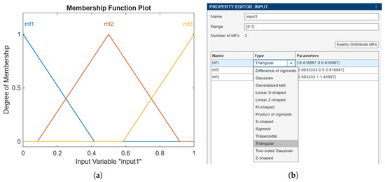
Figure 4.
Configuration of fuzzy system member ship functions: (a) Membership function visualization; (b) Membership function property editor.
In FLCs, membership functions (MFs) play a fundamental role in quantifying the degree of truth associated with linguistic variables. The shape and type of these functions directly impact the controller’s performance, interpretability, and computational efficiency. A wide range of MF types—such as triangular, trapezoidal, Gaussian, bell-shaped, sigmoidal, and others—can be employed, each offering distinct advantages depending on the application’s complexity and dynamic behavior [28].
In this study, triangular and trapezoidal membership functions were primarily adopted due to their simplicity, ease of implementation, and high interpretability. These functions are defined by linear segments, which not only reduce computational overhead but also facilitate real-time execution and straightforward manual tuning—key factors in practical control applications.
Although alternative MF shapes—such as Gaussian, generalized bell, S-shaped, Z-shaped, and singleton functions—were considered during preliminary evaluations, they were ultimately not selected for the final implementation. These alternatives, while offering smoother transitions and potential improvements in modeling nonlinearities, presented disadvantages in this context, including increased computational cost, less intuitive parameter tuning, and a general need for optimization algorithms or empirical adjustments to achieve satisfactory performance.
Given the characteristics of the system under study and the control objectives, the use of triangular and trapezoidal membership functions provided an optimal balance between efficiency, transparency, and control effectiveness. Their use contributed to the overall robustness and clarity of the controller design, without introducing unnecessary complexity.
The rule base, shown in Figure 5, is constructed using the Rule Editor, where individual rules can be defined by selecting appropriate fuzzy sets and logical connectors. This modular interface facilitates the creation of interpretable and flexible control logic.
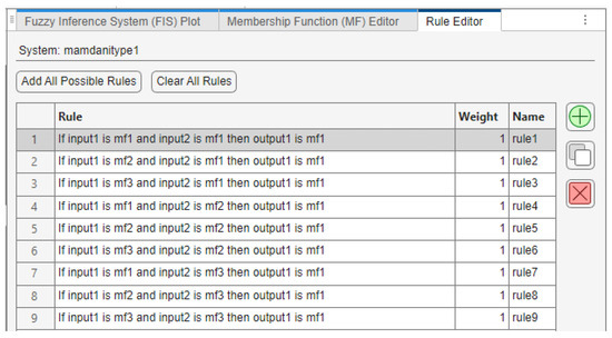
Figure 5.
Fuzzy rule base defined in the MATLAB Rule Editor.
The fuzzy controller was refined using empirical domain knowledge, by adjusting the fuzzy intervals and tuning the membership function values for each input parameter.
After configuration, the fuzzy system can be simulated to evaluate rule inference and visualize the control surface. The toolbox includes a suite of visualization tools that allow users to explore how the system responds to varying input conditions and to examine the resulting control outputs in three dimensions. Overall, the MATLAB Fuzzy Logic Toolbox provides an accessible and robust platform for the design, tuning, and evaluation of fuzzy controllers in both academic and industrial settings.
4.3. Tune PID Controller
Proportional–Integral–Derivative (PID) controllers are among the most widely used feedback control strategies for minimizing the error between a desired setpoint and the system output. The control law in the Laplace domain is defined as
where , and represent the proportional, integral, and derivative gains, respectively.
In this study, the tuning of the , and gains for the classical PID controller was carried out using MATLAB’s “Tuner PID” tool [29], which automatically adjusts the parameters based on the system model to achieve a desired trade-off between performance and robustness. The tool employs internal optimization algorithms, typically based on closed-loop response criteria such as settling time, overshoot, and integral error indices.
4.4. Performance Metrics
Evaluating the control error is essential for assessing the performance of a feedback control system. One widely adopted approach involves the use of integral-based error criteria, which quantify the cumulative error over time in closed-loop operation [30]. These performance indices provide insights into the system’s ability to minimize deviations from the desired output and are especially useful for comparing different control strategies. The principal indices include the following:
- Integral of Squared Error (ISE): Emphasizes larger deviations by penalizing the square of the error, promoting faster correction:
- Integral of Time-weighted Squared Error (ITSE): Penalizes errors that persist over time, encouraging faster stabilization:
- Integral of Absolute Error (IAE): Applies equal weight to all errors regardless of magnitude, often resulting in smoother control actions:
- Integral of Time-weighted Absolute Error (ITAE): Gives higher penalties to long-duration errors, favoring reduced settling time and overshoot:
The application of error indices ISE, IAE, and ITSE in the tuning of fuzzy controllers represents a significant advantage over classical PID controllers, especially in nonlinear and dynamic systems. These indices provide clear metrics that enable automatic and adaptive optimization of the fuzzy controller, resulting in enhanced robustness, flexibility, and improved performance [31,32].
5. Simulations and Results
This section presents the practical results obtained through the implementation and simulation of the control strategies investigated in this work. Using MATLAB/Simulink, various controllers were evaluated, beginning with a conventional PID approach and progressively incorporating more advanced techniques, culminating in a robust Fuzzy Logic Controller. Each control scheme was assessed based on both quantitative performance metrics and qualitative analysis of the system’s dynamic response. Furthermore, in Section 6 a practical case study involving external disturbances was conducted to evaluate the controllers’ robustness and validate their effectiveness in realistic operating conditions.
5.1. Comparison Between Fuzzy Gain Scheduling Controller and Classical PID Controllers
The controllers were tuned according to the system objectives, namely improving both transient and steady-state responses while minimizing the effects of delays inherent to thermal processes. Additionally, the system’s graphical responses and error metrics were analyzed, and the fuzzy intervals and rule base were fine-tuned through iterative simulations. A reference temperature of 18 °C was selected, as it represents a realistic indoor comfort level in typical thermal control applications, such as residential heating, although the system is capable of operating within a 15–30 °C range. For consistency, all fuzzy controller variants (P, PI, PD, and PID) used the same “Error” membership functions, as detailed in Table 1. Each simulation was run for a total duration of 3000 s to capture both transient and steady-state behavior of the thermal system. In line with the Practical Case Study (Section 6), a disturbance signal was applied at 1500 s. Therefore, the simulation time was doubled to allow for a thorough evaluation of the controller’s response to the applied disturbance and to facilitate a more comprehensive analysis of system behavior.

Table 1.
Error input values.
A comparative analysis was conducted between classical controllers and their corresponding Fuzzy Logic implementations to evaluate their performance and advantages in systems with significant time delays. A series of simulations was carried out to iteratively tune controller parameters based on error metrics and time-domain response characteristics. A reference temperature of 18 °C was selected to represent a typical indoor comfort setpoint.
To ensure consistency across Fuzzy controller variants, namely Fuzzy P, PI, PD, and PID, the same membership functions were applied to the “Error” input variable, as detailed in Table 1. The range of error input values reflects the dynamic deviation between the process variable and the desired temperature setpoint throughout the system’s operation. At the initial stage of the response, the error reaches its maximum value, corresponding to the full difference between the initial temperature and the reference value. As the system progresses toward the setpoint, the error gradually decreases to zero. These limits were defined to ensure that the fuzzy inference system effectively covers the entire operating range, enabling adaptive tuning of the proportional, integral, and derivative gains (, , ) be adaptively tuned according to the magnitude of the error.
Each simulation was executed over a 3000 s interval to capture both transient and steady-state behavior.
It is important to note that the output membership functions for each controller variant (P, PI, PD, and PID) were individually tailored. Multiple iterations were required to optimize these functions and ensure appropriate control actions across the different system dynamics.
5.1.1. Fuzzy-PD vs. PD Controllers
The initial comparative analysis involved Proportional-Derivative (PD) control, evaluating both conventional and fuzzy implementations, as illustrated in Figure 6. In this configuration, the value “1” in the diagram represents the derivative filter coefficient (NN), which can significantly influence system dynamics. A larger NN enhances the speed of the derivative response but increases sensitivity to measurement noise, whereas a smaller NN smooths the response at the cost of responsiveness. For this study, a conservative value of was adopted, as it had minimal influence on system performance while reducing computational complexity during simulation.
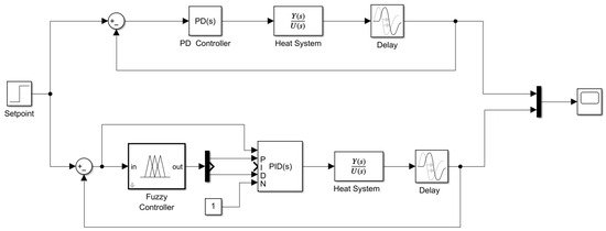
Figure 6.
Block diagram for PD and Fuzzy-PD controllers.
Note that the Demux connection for the integral component (I) is intentionally omitted, as this configuration focuses exclusively on proportional and derivative control actions. Only the corresponding gains ( and ) are considered in this setup.
The proportional component (P) provides control output in direct proportion to the current error. However, in systems with significant delay, a pure P controller typically fails to eliminate the steady-state error unless high gain values are used, which may lead to instability. The proportional gain for the classical P controller was set to , as obtained via the MATLAB PID Tuner.
For the Fuzzy-P controller, the output membership function for was defined using three linguistic terms, with parameters summarized in Table 2.
Table 2.
: Fuzzy-P output values.
The corresponding rule base for the Fuzzy-P controller is shown in Figure 7.
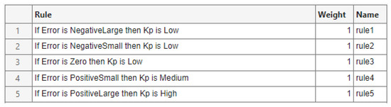
Figure 7.
Fuzzy-P controller rule base.
The derivative component (D) contributes by reacting to the rate of change of the error, thus attenuating oscillations and improving system stability. This is particularly beneficial in systems with delays, where anticipatory action is critical. The Fuzzy-PD controller included a second output membership function for , whose parameters are given in Table 3.
Table 3.
: Fuzzy-PD output values.
The Fuzzy-PD rule base is depicted in Figure 8.
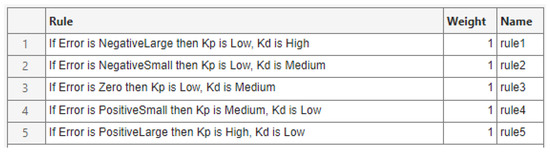
Figure 8.
Fuzzy-PD controller rule base.
The output membership function parameters for were refined through multiple iterations based on step response analysis, with the objective of minimizing overshoot and improving transient behavior. The classical PD controller was configured with and , also determined via the PID Tuner, to serve as a baseline for comparison.
As illustrated in Figure 9, the derivative action significantly reduces the overshoot associated with the proportional term. However, both PD configurations exhibit a persistent steady-state error, suggesting that additional integral action may be required to eliminate long-term offset. Consequently, further experiments were conducted to explore improved control performance with PI and PID configurations.
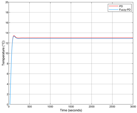
Figure 9.
Step response comparison: Fuzzy-PD vs. classical PD (reference = 18 °C).
5.1.2. Fuzzy-PI vs. PI Controllers
The second experiment involved replacing the derivative action (D) with integral action (I) in both controllers, as illustrated in the block diagram shown in Figure 10.
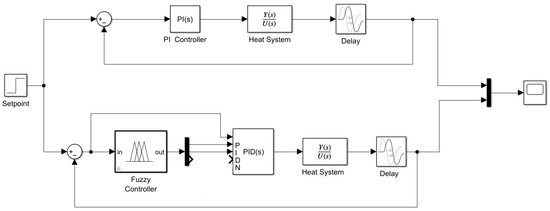
Figure 10.
Block diagram: Fuzzy-PI vs. classical PI controller.
It is worth noting that, as mentioned in the previous section for the PD controller, the Demux connection for the derivative component (D) is intentionally omitted, as this configuration focuses exclusively on proportional and integral control actions. Only the corresponding gains ( and ) are considered in this setup.
The primary function of integral action is to eliminate steady-state error by accumulating the error over time. In systems characterized by delays, where proportional control alone may be insufficient, the integral term ensures convergence to zero error. The integral gain was set to , obtained using the PID Tuner, while the proportional gain remained unchanged at .
For the Fuzzy-PI controller, the initial values for the output membership function corresponding to are presented in Table 4.
Table 4.
: Fuzzy-PI output values.
The rule base applied to the Fuzzy-PI controller is illustrated in Figure 11.
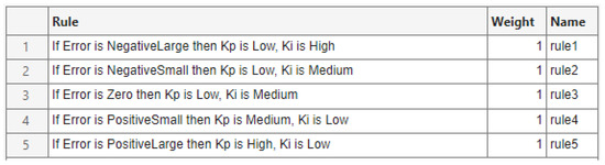
Figure 11.
Fuzzy-PI controller rule base.
The corresponding step responses of both controllers are shown in Figure 12.

Figure 12.
Step response comparison: Fuzzy-PI vs. PI.
Quantitative performance metrics—including rise time, settling time, overshoot, and steady-state error, were extracted using Simulink’s “To Workspace” block in conjunction with MATLAB’s stepinfo() function. The results are summarized in Table 5.
Table 5.
Time metrics comparison between Fuzzy-PI and PI controllers.
In addition, classical performance indices, particularly the integral-based error metrics, were calculated from the simulation data. While the error response plots are omitted for conciseness, the respective values were extracted directly using MATLAB. Table 6 presents a comparative summary of these metrics.
Table 6.
Performance metric comparison between Fuzzy-PI and PI controllers.
Based on the results in Table 5, the Fuzzy-PI controller demonstrated a faster rise time and a shorter settling time compared to the classical PI controller. While it exhibited a slightly higher overshoot, both overshoot values remained below , indicating a well-damped response in both cases. Furthermore, both controllers achieved zero steady-state error.
The performance indices in Table 6 further confirm that the Fuzzy-PI controller outperforms the classical PI controller across all evaluated metrics, with consistently lower error values.
In conclusion, the Fuzzy-PI approach demonstrated superior performance compared to the classical PI controller, both in terms of transient response and cumulative error metrics.
5.1.3. Fuzzy-PID vs. PID Controllers
The third and final experiment incorporated all three control actions, proportional (P), integral (I), and derivative (D), resulting in the complete control structure shown in Figure 13.
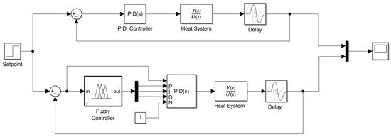
Figure 13.
Block diagram: Fuzzy-PID vs. classical PID controller.
As the values of , and for both the fuzzy and classical controllers had already been established in the previous experiments, the final configuration simply required integrating all components. The only modification involved expanding the fuzzy rule base to incorporate all three control terms, as illustrated in Figure 14.
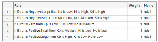
Figure 14.
Fuzzy-PID rule base.
The resulting step responses for both controllers are presented in Figure 15.
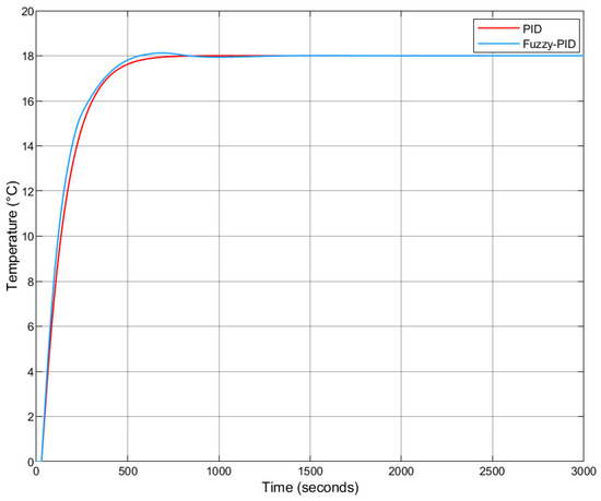
Figure 15.
Step response comparison: Fuzzy-PID vs. PID.
Time-domain performance metrics are summarized in Table 7.
Table 7.
Time metrics comparison between Fuzzy-PID and PID controllers.
The classical performance indices were computed based on simulation results. The corresponding values are shown in Table 8.
Table 8.
Performance metric comparison between Fuzzy-PID and PID controllers.
It is important to clarify that the performance indices (ISE, IAE, ITSE, and ITAE) were not employed during the design or tuning of the fuzzy membership functions. For all controller configurations (PD, PI, and PID), the fuzzy sets and rule bases were refined empirically through iterative simulations, with a primary focus on improving transient and steady-state behavior. Only after achieving satisfactory dynamic responses, the performance indices were computed to quantitatively assess and compare the final behavior of each classical controller and its corresponding Fuzzy variant. This approach ensures that the reported metrics objectively reflect the closed-loop performance, without biasing the initial design process of the fuzzy inference system.
As shown in Table 7, the Fuzzy-PID controller achieved a faster rise time and shorter settling time compared to the classical PID controller, albeit with a slightly higher overshoot. However, the overshoot remained under 1% in both cases, indicating a well-damped response. Both controllers eliminated steady-state error completely.
Furthermore, as indicated in Table 8, the Fuzzy-PID controller outperformed its classical counterpart in all performance indices, exhibiting lower cumulative error values.
In summary, the Fuzzy-PID controller consistently demonstrated superior performance relative to the classical PID controller, both in terms of transient response and overall error minimization.
5.2. Impact of Anti-Windup Compensation in Time-Delay Control Systems
To mitigate integrator windup caused by actuator saturation, an anti-windup scheme was implemented based on the back-calculation method. This approach introduces a corrective feedback signal proportional to the discrepancy between the saturated and unsaturated control outputs, scaled by a tuning parameter, . This error signal is divided by the anti-windup time constant and then fed back into the integrator, effectively limiting the accumulation of the integral term during saturation events. The anti-windup time constant is defined as: . The parameter governs the responsiveness of the anti-windup compensation: lower values result in slower recovery dynamics, whereas higher values may induce oscillatory behavior.
The subsequent subsections detail the implementation of anti-windup mechanisms in PI and PID controller configurations.
5.2.1. Anti-Windup in Fuzzy-PI and PI Controllers
The initial comparative analysis involved Proportional-Integrative (PI) control, evaluating both conventional and fuzzy implementations. The control architecture incorporating the anti-windup mechanism is illustrated in Figure 16.
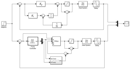
Figure 16.
Block diagram: Fuzzy-PI vs. PI with Anti-Windup implementation.
Tests were conducted with a actuator saturation limit and different values of (0.5, 1.0, and 1.5). As shown in Figure 17, the anti-windup mechanism did not yield significant performance improvements for the thermal system under consideration. In some cases, it even introduced additional oscillations or increased overshoot, Figure 17a.
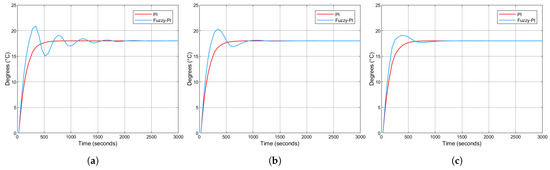
Figure 17.
Step response comparison: Fuzzy-PI vs. PI with Anti-Windup for different values—(a) , (b) , (c) .
5.2.2. Anti-Windup in Fuzzy-PID and PID Controllers
An additional test was performed by incorporating derivative action into the controllers. However, this modification did not produce any significant improvement in the anti-windup response, following what was observed in the Fuzzy-PI and PI configurations (Figure 17). Therefore, the use of anti-windup mechanisms in the Fuzzy-PID and PID controllers was excluded from further analysis.
5.3. Smith Predictor in Fuzzy-PI and Fuzzy-PID Controllers
This subsection presents the final set of experiments, which evaluate the impact of incorporating a Smith Predictor into both the Fuzzy-PI and Fuzzy-PID controllers, as well as into their conventional counterparts, the PI and PID controllers.
The Smith Predictor is a model-based control strategy that compensates for time delays by predicting future plant outputs using a mathematical model of the process. This enables the controller to respond as if no delay were present, thereby improving system responsiveness and reducing oscillations [33].
5.3.1. Fuzzy-PI with Smith Predictor vs. PI with Smith Predictor
The first experiment evaluated the impact of integrating a Smith Predictor into both the Fuzzy-PI and PI controllers.
The updated block diagram for this configuration is presented in Figure 18.

Figure 18.
Block diagram: Fuzzy-PI vs. PI with Smith Predictor.
The corresponding step responses are shown in Figure 19.
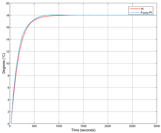
Figure 19.
Step response comparison: Fuzzy-PI vs. PI with Smith Predictor.
Table 9 summarizes the time-domain metrics. The results demonstrate that the Fuzzy-PI controller outperforms the classical PI controller by achieving a faster rise time and a shorter settling time. Although the Fuzzy-PI controller exhibits a slightly higher overshoot, both values remain below , indicating a well-damped system response. Both controllers successfully eliminated the steady-state error.
Table 9.
Time metrics comparison between Fuzzy-PI and PI controllers with Smith Predictor implementation.
Compared to their respective configurations without the Smith Predictor, both controllers showed an increase in settling time, approximately 74 s for Fuzzy-PI and 110 s for PI. However, the Fuzzy-PI controller with Smith Predictor still reached stability around 73 s faster than the PI controller with the same predictive structure.
To further support the analysis, classical performance indices were evaluated and are presented in Table 10.
Table 10.
Performance metrics comparison between Fuzzy-PI and PI controllers with and without Smith Predictor.
Although the inclusion of the Smith Predictor leads to slightly higher total error values, the key benefit lies in the reduction of oscillations and a smoother control response, which justifies its application, particularly in systems with significant time delays.
5.3.2. Fuzzy-PID with Smith Predictor vs. PID with Smith Predictor
The second experiment involving the Smith Predictor was conducted using PID-based controllers, as illustrated in the block diagram in Figure 20.
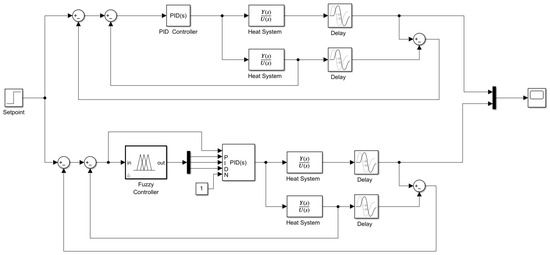
Figure 20.
Block diagram: Fuzzy-PID vs. PID with Smith Predictor.
The corresponding step responses are presented in Figure 21.
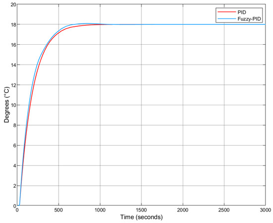
Figure 21.
Step response comparison: Fuzzy-PID vs. PID with Smith Predictor.
Table 11 summarizes the time-domain metrics. The results show that the Fuzzy-PID controller achieves a faster rise time and shorter settling time compared to the classical PID controller. While the Fuzzy-PID displays a slightly higher overshoot, both overshoot values remain below , indicating well-damped system behavior. Moreover, both controllers achieve zero steady-state error.
Table 11.
Time metrics comparison between Fuzzy-PID and PID controllers with Smith Predictor implementation.
Compared to the configurations without the Smith Predictor, both controllers exhibit increased settling times, approximately 87 s for the Fuzzy-PID and 111 s for the PID. Nonetheless, the Fuzzy-PID with Smith Predictor still reaches steady-state about 66 s faster than its PID counterpart under the same configuration.
To further support the analysis, classical performance indices were evaluated and are presented in Table 12.
Table 12.
Performance metrics comparison between Fuzzy-PID and PID controllers with and without Smith Predictor.
Although the integration of the Smith Predictor results in slightly increased error metrics compared to configurations without it, the conclusions remain consistent with those drawn for the PI configurations: the overall benefit lies in the reduction of oscillations and the improved smoothness of the system response. These advantages justify the inclusion of the Smith Predictor, particularly in systems where accurate delay compensation is critical.
5.4. Choice of Controller Type
The Fuzzy-PID controller was selected for its optimal balance between fast transient response, steady-state accuracy, and robustness to delays and disturbances. This choice is consistent with the study’s objective of identifying a practical and adaptable control architecture for thermal systems. Based on the simulation results, both Fuzzy-PI/PI and Fuzzy-PID/PID controllers, with and without the Smith Predictor, are viable solutions for controlling systems with time delays. Although the Fuzzy-PI and PI controllers demonstrated marginally lower steady-state error values, the Fuzzy-PID and PID controllers provided faster and smoother transient responses. Considering the negligible differences in steady-state errors alongside the improved dynamic performance, the Fuzzy-PID and PID configurations were selected for further investigation in the practical case study presented in Section 6.
6. Practical Case Study
To further validate the comparison between the Fuzzy-PID and PID controllers, a more realistic simulation scenario was introduced by incorporating external disturbances. Specifically, a noise block was added to simulate environmental events such as door or window openings while the system aims to maintain an indoor temperature of 18 °C. These disturbances mimic sudden exposure to extreme outdoor conditions.
A custom noise block was developed to inject random disturbances, both positive and negative, after the system reaches a steady state, as illustrated in Figure 22.
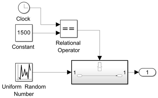
Figure 22.
Noise model components.
To evaluate robustness, both the Fuzzy-PID and PID controllers were tested with and without the Smith Predictor under identical noise conditions. Disturbances were introduced at 1500 s, after the system had stabilized.
6.1. Noise Implementation Without Smith Predictor
Using the same block diagram structure described in Section 5.1.3, the only modification was the addition of the noise block at the heat system input.
Two disturbance scenarios were analyzed:
- Elevated external temperatures, where the ambient temperature exceeds the setpoint.
- Reduced external temperatures, where the ambient temperature falls below the setpoint.
The system’s response under warmer external conditions is shown in Figure 23.
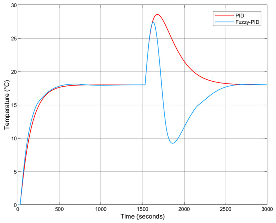
Figure 23.
Fuzzy-PID vs. PID step response under warmer external temperatures (no Smith Predictor).
Under colder external temperatures, the response is shown in Figure 24.
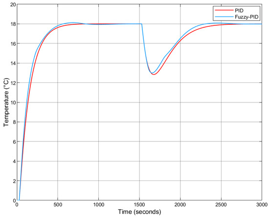
Figure 24.
Fuzzy-PID vs. PID step response under colder external temperatures (no Smith Predictor).
To streamline the analysis, only the “Warmer Temperatures” scenario was used to compute performance metrics, as it exhibited more pronounced variations. As expected, the introduction of noise resulted in increased error values due to the need for corrective action. The computed performance indices are shown in Table 13.
Table 13.
Performance metric comparison between Fuzzy-PID and PID controllers with noise.
Following the structure described in Section 5.3.2, this implementation also incorporated the noise block. Again, two scenarios were analyzed.
The response under warmer external temperatures is shown in Figure 25.
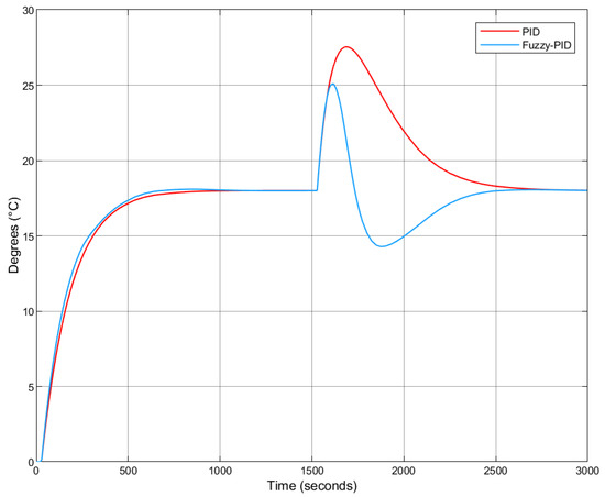
Figure 25.
Fuzzy-PID vs. PID step response under warmer external temperatures (with Smith Predictor).
The response under colder external temperatures is presented in Figure 26.
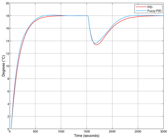
Figure 26.
Fuzzy-PID vs. PID step response under colder external temperatures (with Smith Predictor).
As before, performance metrics were calculated only for the warmer temperature scenario. The results are summarized in Table 14.
Table 14.
Performance metric comparison between Fuzzy-PID and PID controllers with noise and Smith Predictor implementation.
6.2. Comparison Between Implementations
The analysis of controller responses to noise disturbances reveals that both Fuzzy-PID and classical PID controllers effectively compensate to restore the system to the desired setpoint. However, the Fuzzy-PID controller consistently outperforms the PID controller by achieving faster convergence to the target value.
Regarding the Smith Predictor implementation, it is observed that this model-based compensation not only results in a smoother system response but also enables quicker controller action with reduced overshoot. A comparison between Figure 23 and Figure 25, which illustrate responses under “Warmer Temperatures Noise” conditions, highlights the superior performance of the Smith Predictor-enhanced system in terms of both response time and stability.
Moreover, error metrics further confirm the advantage of the Fuzzy-PID approach, which maintains lower error values compared to the classical PID controller.
In conclusion, the combination of the Fuzzy-PID controller with the Smith Predictor yields the most favorable control performance among the configurations evaluated.
7. Conclusions
This study conducted a comparative analysis of classical PID and fuzzy logic-based control strategies applied to a heat diffusion system with inherent time delay. Among the evaluated configurations, including Fuzzy-P, Fuzzy-PD, Fuzzy-PI, and Fuzzy-PID, the Fuzzy-PID controller demonstrated the optimal balance between dynamic performance, stability, and robustness. Although the Fuzzy-PI and PI controllers achieved satisfactory steady-state accuracy. The inclusion of derivative action markedly enhanced transient response by reducing rise time, settling time, and overshoot.
Additional control enhancements, namely Anti-Windup and the Smith Predictor, were also assessed. While the Anti-Windup mechanism showed no significant benefit in this application, the Smith Predictor effectively improved disturbance rejection and overall robustness.
As a future research direction, the practical implementation of the proposed control strategy on a real thermal system is planned. Owing to the relatively low computational complexity of the developed control scheme—particularly due to the use of triangular and trapezoidal membership functions—the approach is highly suitable for deployment on low-cost resource constrained embedded hardware platforms. This step will enable real-time validation under realistic operating conditions, including sensor noise, actuator nonlinearities, and sampling limitations. Such an implementation will offer valuable insights into the controller’s robustness, responsiveness, and overall feasibility in embedded environments, further supporting its applicability to a broader class of systems with varying time delays and environmental conditions in both industrial and educational settings.
In summary, the integration of a Fuzzy-PID controller with a Smith Predictor provides the most effective and robust control solution for the thermal system under investigation.
Author Contributions
Conceptualization, R.S.M. and I.S.J.; methodology, R.S.M. and I.S.J.; software, R.S.M.; validation, R.S.M. and I.S.J.; formal analysis, R.S.M. and I.S.J.; investigation, R.S.M. and I.S.J.; writing—original draft preparation, R.S.M.; writing—review and editing, R.S.M. and I.S.J.; visualization, R.S.M.; supervision, I.S.J. All authors have read and agreed to the published version of the manuscript.
Funding
This research received no external funding.
Data Availability Statement
The original contributions presented in this study are included in the paper. Further inquiries can be directed to the corresponding author.
Conflicts of Interest
The authors declare no conflicts of interest.
References
- Ogata, K. Modern Control Engineering; Prentice Hall: Upper Saddle River, NJ, USA, 2022; ISBN 0136156738. [Google Scholar]
- Myronchuk, Y.; Khmelniuk, M. Temperature Waves Phase Optimal Time Lag in the Refrigerated Warehouse Thermal Insulation. Gazi Univ. J. Sci. 2022, 35, 1102–1114. [Google Scholar] [CrossRef]
- Liu, C.; Loxton, R.; Teo, K.L.; Wang, S. Optimal state-delay control in nonlinear dynamic systems. Autom. J. 2022, 135, 109981. [Google Scholar] [CrossRef]
- Jensen, C.M.; Frederiksen, M.C.; Kallesøe, C.S.; Jensen, J.N.; Andersen, L.H.; Izadi-Zamanabadi, R. HAVOK Model Predictive Control for Time-Delay Systems with Applications to District Heating; IFAC-Papers OnLine; Elsevier: Amsterdam, The Netherlands, 2023; Volume 56, pp. 2238–2243. [Google Scholar] [CrossRef]
- Vivek, R.; Abdelfattah, W.M.; Elsayed, E.M. Analysis of Delay-Type Integro-Differential Systems Described by the Φ-Hilfer Fractional Derivative. Axioms J. 2025, 14, 629. [Google Scholar] [CrossRef]
- Ma, Y.; Borrelli, F.; Hencey, B.; Coffey, B.; Bengea, S.; Haves, P. Model Predictive Control for the Operation of Building Cooling Systems. IEEE Trans. Control Syst. Technol. 2009, 20, 796–803. [Google Scholar] [CrossRef]
- Wang, L. Model Predictive Control System Design and Implementation Using MATLAB; Springer: Berlin, Germany, 2003. [Google Scholar] [CrossRef]
- Venkatachalam, V.; Ramasubramanian, M.; Thirumarimurugan, M.; Prabhakaran, D. Computation of Time Delay for Delayed Network Controlled Temperature Control System. J. Phys. 2021, 2070, 012102. [Google Scholar] [CrossRef]
- Gemechu, D.A.; Prabakaran, K.; N, L.; Nagarajan, S.; Umamaheswaran, S.; S, U.; Feyisa, M.L. Stability Results of Thermal Control System with Time-Dependent Delays and Perturbations of Nonlinearity. J. Adv. Mater. Sci. Eng. 2022, 2022, 4486756. [Google Scholar] [CrossRef]
- Seborg, D.E.; Edgar, T.F.; Mellichamp, D.A.; Doyle, F.J., III. Process Dynamics and Control, 3rd ed.; Wiley: Hoboken, NJ, USA, 2010; ISBN 9780470128671. [Google Scholar]
- Åström, K.J.; Hägglund, T. PID Controllers; International Society for Measurement and Control: London, UK, 1995; p. 343. ISBN 1556175167. [Google Scholar]
- Marlin, T.E. Process Control: Designing Processes and Control Systems for Dynamic Performance, 2nd ed.; McGraw-Hill: New York, NY, USA, 2015. [Google Scholar]
- Zadeh, L.A. Fuzzy Logic = Computing with Words. IEEE Trans. Fuzzy Syst. 1996, 4, 103–111. [Google Scholar] [CrossRef]
- Deshpande, P.B.; Ash, R.H. Elements of Computer Process Control, with Advanced Control Applications; Instrument Society of America: Pittsburgh, PA, USA, 1981. [Google Scholar]
- Gerald, C.F.; Wheatley, P.O. Applied Numerical Analysis, 7th ed.; Pearson College Div: Metchosin, BC, Canada, 2003. [Google Scholar]
- Incropera, F.P.; DeWitt, D.P. Fundamentals of Heat and Mass Transfer, 4th ed.; John Wiley & Sons: New York, NY, USA, 1996; ISBN 9780471304609. [Google Scholar]
- Cengel, Y.A. Heat Transfer: A Practical Approach, 2nd ed.; McGraw Hill: Columbus, OH, USA, 2022; Available online: https://pt.scribd.com/doc/76358132/Heat-Transfer-Yunus-a-Cengel-2nd-Edition (accessed on 23 September 2025).
- Narasimhan, T.N. Fourier’s Heat Conduction Equation: History, Influence, and Connections. Rev. Geophys. 1999, 37, 151–172. [Google Scholar] [CrossRef]
- Lienhard, J.H. A Heat Transfer Textbook, 5th ed.; Phlogiston Press: Cambridge, MA, USA, 2020; Available online: http://ahtt.mit.edu (accessed on 23 September 2025).
- Nise, N.S. Control Systems Engineering, 6th ed.; Wiley: Hoboken, NJ, USA, 2011. [Google Scholar]
- Zimmermann, H.-J. Fuzzy Set Theory and Its Applications; Springer: Dordrecht, The Netherlands, 2001. [Google Scholar] [CrossRef]
- Passino, K.M.; Yurkovich, S. Fuzzy Control; Addison-Wesley: Boston, MA, USA, 1998; p. 475. ISBN 020118074X. [Google Scholar]
- Castillo, O.; Melin, P. A Classification of Fuzzy Controllers. 2013. Available online: https://www.researchgate.net/figure/A-classification-of-fuzzy-controllers_fig1_255567860 (accessed on 13 May 2025).
- Kovačić, Z.; Bogdan, S. Fuzzy Controller Design Theory and Applications; Taylor & Francis: New York, NY, USA, 2006. [Google Scholar]
- Widrow, B. Intelligent Control Nazmul Siddique: A Hybrid Approach Based on Fuzzy Logic, Neural Networks and Genetic Algorithms; Foreword by Bernard Widrow; Springer: Berlin/Heidelberg, Germany, 2014; Available online: http://www.springer.com/series/7092 (accessed on 23 September 2025).
- Jesus, I.S.; Machado, J.A.T.; Barbosa, R.S. On the Fractional Order Control of Heat Systems. In Intelligent Engineering Systems and Computational Cybernetics; Machado, J.A.T., Pátkai, B., Rudas, I.J., Eds.; Springer: Dordrecht, The Netherlands, 2009; pp. 375–385. [Google Scholar] [CrossRef]
- The MathWorks, Inc. Fuzzy Logic Toolbox User’s Guide; MathWorks: Natick, MA, USA, 2023; Available online: https://www.mathworks.com/products/fuzzy-logic.html (accessed on 23 September 2025).
- Cirstea, M.N.; Dinu, A.; Khor, J.G.; Mc Cormick, M. Neural and Fuzzy Logic Control of Drives and Power Systems; Springer: Berlin/Heidelberg, Germany, 2002. [Google Scholar] [CrossRef]
- MathWorks. PID Tuner—Tune PID Controllers; The MathWorks, Inc.: Natick, MA, USA, 2025; Available online: https://www.mathworks.com/help/control/ref/pidtuner-app.html (accessed on 18 May 2025).
- Dorf, R.C.; Bishop, R.H. Modern Control Systems, 13th ed.; Pearson: London, UK, 2016; ISBN 9780134407623. [Google Scholar]
- Das, S.; Pan, I.; Das, S.; Gupta, A. A novel fractional order fuzzy PID controller and its optimal time domain tuning based on integral performance indices. Eng. Appl. Artif. Intell. J. 2012, 25, 430–442. [Google Scholar] [CrossRef]
- Othman, S.B.; Ramdas, S.K. Robust Fuzzy-PID Technique for the Automatic Generation Control of Interconnected Power System with Integrated Renewable Energy. Eur. J. Electr. Eng. Comput. Sci. 2024, 8, 21–31. [Google Scholar] [CrossRef]
- İçmez, Y.; Can, M.S. Smith Predictor Controller Design Using the Direct Synthesis Method for Unstable Second-Order and Time-Delay Systems. Processes 2023, 11, 941. [Google Scholar] [CrossRef]


Disclaimer/Publisher’s Note: The statements, opinions and data contained in all publications are solely those of the individual author(s) and contributor(s) and not of MDPI and/or the editor(s). MDPI and/or the editor(s) disclaim responsibility for any injury to people or property resulting from any ideas, methods, instructions or products referred to in the content. |
© 2025 by the authors. Licensee MDPI, Basel, Switzerland. This article is an open access article distributed under the terms and conditions of the Creative Commons Attribution (CC BY) license (https://creativecommons.org/licenses/by/4.0/).