Abstract
The Hamiltonian Monte Carlo (HMC) method is effective for Bayesian inference but suffers from synchronization overhead in distributed settings. We propose two variants: a distributed HMC (DHMC) baseline with synchronized, globally exact gradient evaluations and a communication-avoiding leapfrog HMC (CALF-HMC) method that interleaves local surrogate micro-steps with a single–global Metropolis–Hastings correction per trajectory. Implemented on Apache Spark/PySpark and evaluated on a large synthetic logistic regression (, , workers ), DHMC attained an average acceptance of , mean ESS of 1200, and wall-clock of s per evaluation run, yielding ESS/s; CALF-HMC achieved an acceptance of , mean ESS of , and s, i.e., ≈0.34 ESS/s under the tested surrogate configuration. While DHMC delivered higher ESS/s due to robust mixing under conservative integration, CALF-HMC reduced the per-trajectory runtime and exhibited more favorable scaling as inter-worker latency increased. The study contributes (i) a systems-oriented communication cost model for distributed HMC, (ii) an exact, communication-avoiding leapfrog variant, and (iii) practical guidance for ESS/s-optimized tuning on clusters.
1. Introduction
Markov Chain Monte Carlo (MCMC) simulation refers to several techniques for sampling from unknown or difficult-to-sample-from probability distributions. The basic concept is that with a clever transition rule, a Markov chain can be used to sample from a complicated distribution. This has led to a so-called ‘revolution’ in the sciences, with computational papers in many fields opting to use it [1]. This study will exposit the background and content of the most popular MCMC methods. The methods and diagnostic tools for carrying out real-world experiments will be covered as well. The final chapters will attempt to go beyond theory and look at the developments that have enabled MCMC simulation to become commonplace in the sciences, as well as conducting an original investigation. We begin with a background on the mathematics of Markov chains.
Modern applications illustrate this breadth, spanning computational statistics, machine learning, and safety-critical domains such as industrial control systems (ICS) cybersecurity. For example, model-based systems engineering (MBSE) approaches that operationalize the NIST Risk Management Framework (RMF) for ICS adopt probabilistic modeling and Bayesian reasoning to support risk assessment and decision making [2]. Complementary surveys and systems-oriented studies highlight scalable MCMC via stochastic-gradient dynamics, subsampling, factorized acceptance, and distributed consensus [3,4,5,6].
Recent advancements in scalable Markov Chain Monte Carlo (MCMC) methods have significantly improved the efficiency of Bayesian inference in large-scale and high-dimensional data contexts. Fearnhead et al. provided an extensive discussion on contemporary approaches such as stochastic gradient MCMC and continuous-time dynamics, which have become essential in addressing the computational challenges posed by modern machine learning tasks [3]. Similarly, Korattikara introduced approximate MCMC techniques, including the Stochastic Gradient Langevin Dynamics (SGLD), which enable mini-batch processing to scale Bayesian inference while mitigating overfitting [7]. In line with this, Strathmann et al. proposed a methodology using partial posteriors to bypass full posterior simulation, offering unbiased estimates and sub-linear complexity [8]. Pollock et al. further contributed by presenting the Scalable Langevin Exact Algorithm, which bypasses traditional Metropolis–Hastings steps, achieving computational gains through innovative subsampling strategies [9].
Cornish et al. introduced the Scalable Metropolis–Hastings (SMH) kernel, which achieves efficient Bayesian inference by reducing the per-iteration cost and maintaining posterior accuracy through factorized acceptance mechanisms and fast Bernoulli processes [4]. Their approach ensures geometric ergodicity and has shown consistent improvements over classical methods. Foundational work by Johannes and Polson [10] and Craiu and Rosenthal offer crucial theoretical background on MCMC algorithms but lack direct focus on scalability, underscoring the need for adaptation in big data scenarios [11]. Addressing intractable likelihoods in Markov processes, Owen et al. proposed combining approximate Bayesian computation with MCMC to improve inference efficiency on parallel architectures [12].
The explosive growth of modern data—often summarized by the four Vs of volume, velocity, variety, and veracity—challenges classical Bayesian computation. While Markov Chain Monte Carlo (MCMC) remains the “gold standard” for sampling from complex posteriors, naïvely scaling chains to billions of observations or terabyte-sized state spaces is untenable. This study, therefore, bridges traditional MCMC theory with recent scalable developments that exploit mini-batch gradients, distributed memory, and hardware accelerators.
Recent advances motivate three study axes aligned with prior scalable Bayesian computing [3,4,5,6] described as follows:
- Scalable Bayesian toolbox: Taxonomy of SG–MCMC, subsampling/control variates, distributed/consensus MCMC, SMC, and VI.
- Systems orientation: Mappings to Spark/Ray/JAX to surface communication and memory trade-offs.
- Performance metric: We emphasize ESS/s as a practical joint measure of statistical mixing and systems efficiency.
Novelty and Positioning
The proposed CALF-HMC advances beyond communication-avoiding or surrogate-based MCMC by (i) preserving posterior exactness through a single global Metropolis–Hastings correction per trajectory, (ii) reducing synchronized all-reduces from per leapfrog to per trajectory via local surrogate micro-steps, and (iii) coupling these design choices to an explicit communication cost model that predicts ESS/s trends under varying inter-worker latencies. In contrast to stochastic-gradient MCMC families that trade global exactness for per-iteration speed, as well as to consensus-style aggregation methods that remain approximate, our approach targets synchronization frequency as the primary systems bottleneck while retaining trajectory-level exactness. Scalable Metropolis–Hastings techniques are complementary and may be incorporated to further reduce acceptance–computation costs. This positioning directly connects to contemporary scalable MCMC literature on SG–MCMC, consensus aggregation, and factorized acceptance, and it provides a systems-grounded bridge to distributed implementations on Spark-like platforms.
2. Related Work and Foundations
Markov Chain Monte Carlo (MCMC) methods, since their inception, have revolutionized computational statistics by enabling sampling from complex probability distributions. The foundational work by Metropolis et al. introduced a Monte Carlo algorithm utilizing Markov chains for sampling distributions relevant to statistical physics [13]. This was generalized by Hastings, who formalized the Metropolis–Hastings algorithm, allowing for asymmetric proposal distributions and broadening applications across Bayesian inference [14]. The introduction of the Gibbs sampler by Geman et al., originally developed for image restoration, further extended MCMC’s capability to sample from high-dimensional joint distributions through iterative sampling from conditional distributions [15].
The challenges of scaling MCMC algorithms to modern large and high-dimensional datasets have triggered significant advances in recent years. Notably, Welling and Teh introduced the Stochastic Gradient Langevin Dynamics (SGLD) approach, integrating stochastic gradient methods with Langevin dynamics to allow scalable Bayesian learning via mini-batches [16]. Contemporary developments in scalable MCMC are comprehensively reviewed by Fearnhead et al., highlighting methods based on stochastic gradients and continuous-time dynamics that address the computational burdens of big data [3].
Approximate MCMC algorithms have also been a focus, with Korattikara et al. proposing methods to reduce the Metropolis–Hastings computational budget via subsampling, which is termed austerity in MCMC [17]. Strathmann et al. further contributed unbiased Bayesian inference techniques through partial posteriors, enabling sub-linear complexity in data size [8]. Pollock et al. presented scalable Langevin exact algorithms that avoid traditional Metropolis–Hastings steps using innovative subsampling strategies for exact Bayesian inference [18].
To improve efficiency in Bayesian inference with very large datasets, Cornish et al. developed Scalable Metropolis–Hastings kernels employing factorized acceptance mechanisms and fast Bernoulli processes [4]. An important branch of scalable MCMC involves consensus Monte Carlo (CMC) approaches that partition data, perform local inference on each subset, and combine posterior samples. A representative study by Scott et al. formalized this method, enabling scalable Bayesian analysis through consensus aggregation [5].
More recently, distributed Bayesian inference frameworks tailored to large-scale and Internet-of-Things (IoT) systems have been explored. Vlachou et al. demonstrate distributed Bayesian inference techniques compatible with big data environments pertinent to IoT applications, leveraging modern distributed computing frameworks [6]. Table 1 summarizes the objectives, methods, principal findings, and remaining gaps across prior work.

Table 1.
Representative scalable Bayesian/MCMC studies: objectives, key findings, and identified gaps relative to distributed HMC.
Our work builds on and extends these foundational and state-of-the-art approaches by proposing two novel distributed Hamiltonian Monte Carlo methods—Distributed HMC (DHMC) and Communication-Avoiding Leapfrog HMC (CALF-HMC)—tailored for modern large-scale distributed systems. Unlike many surveys or tutorials that predominantly focus on describing algorithms or comparing classical methods, our study integrates theoretical foundations with practical system-oriented implementations targeting runtime scalability, communication efficiency, and statistical exactness on contemporary big data platforms like Apache Spark. Thus, it bridges MCMC theory with distributed computing infrastructure while providing rigorous experimental evaluation.
3. Markov Chains and Background
3.1. Markov Chains
Markov chains were introduced by Andrey Markov in 1906 in order to prove that the weak law of large numbers does not require strict independence of random variables. In particular, he conducted an experiment where he recorded all of the two-letter bigrams in Pushkin’s Eugene Onegin to demonstrate his property [19]. Whether he intended it or not, Markov chains have since become a powerful modeling tool used across machine learning and Bayesian statistics. In this section, we cover the basic properties of Markov chains and develop the theory necessary to understand MCMC simulation.
The following definitions give explanations for Markov chains on discrete state spaces. The definitions here come from chapter 11 of Markov chains from Introduction to Probability by Blitzstein and Hwang [20], in accordance with other works [21,22].
Definition 1
(Markov Chain, [20]). A sequence of random variables defined on a finite or countable state space or is called a Markov chain if, for all ,
This condition is called the Markov property.
The Markov property states that the probability of transitioning from state i to j when moving from to is only dependent on the fact that . If we consider the variables in the chain to be steps in time, with n representing the step number, then all of the steps before n do not tell us anything about the distribution of .
Definition 2
(Transition matrix, [20]). If is a Markov chain on a countable state space , then the matrix Q with cells is called the transition matrix of the chain.
Note that if the state space is finite with M states, then the dimensions of Q are . If the state space is countably infinite, then Q is not a matrix in the traditional sense but still follows the same rules of addition and multiplication [19].
Proposition 1
(Properties of transition matrices). There are three immediate properties of a transition matrix Q:
- 1.
- Q is non-negative.
- 2.
- , as the rows of Q are conditional probability distributions for given .
- 3.
- The probability of transitioning from i to j after n steps, denoted as , can be represented by the cell of the power .
To see part (3), note that the probability of going from i to j after two steps is , which is the cell of . The case in n steps can be seen by induction [20] (p. 462). Thus, we can say that the conditional distribution for any k is given by the ith row of .
Example 1
(Weather chain). Any day is either sunny, cloudy, or rainy. We can construct the following transition matrix to describe a Markov chain on these states:
Each cell of Q tells us the probability from transitioning from one state to another in one step. For example, if day n is sunny, to see the distribution of possible weather for day , one would look to the first row of Q. In this case, the day has the distribution . To see the probability of going from one state to another over two steps, we can simply compute
Let v be a row vector that describes the starting probability distribution over the state space of a chain, i.e., . Then, Proposition 1 (3) implies that the marginal distribution of is given by . Note that this is different from the conditional distribution, which is simply given by , as noted above in Proposition 1.
Now, we introduce some vocabulary for describing Markov chains.
Definition 3
(Recurrent and transient states, [20]). A state i in the state space of a Markov chain is recurrent if starting from , and the probability of returning to i at some later step is 1. The opposite of recurrent is transient, which means that starting from , there is a positive probability that the future steps will never return to i.
In example 1 we can see that all of the states are recurrent in the weather chain. From any state, it is possible to eventually transition to any other state. Therefore, from any state, the probability of leaving forever is 0, which implies the probability of returning infinitely many times is 1.
From Definition 2, it should be apparent that if state i in a finite state space is transient, then the Markov chain will leave it forever at some point with a probability of 1.
Definition 4
(Reducibility [20]). A chain is said to be irreducible if for all states i and j, there is a positive probability of transitioning from i to j in a finite number of steps. Otherwise, the chain is said to be reducible.
Note that recurrent is a property of a state, and reducible is a property of a Markov chain.
Example 2
(Reducible chain). Consider the four-state Markov chain described by the transition matrix
We can say that states 1 and 2 are transient, as there is a positive probability of never returning to them when starting from them. For example, the probability of transitioning from state 1 to state 3 is . Since from state 3 it is impossible to return to state 1, we know that if the chain starts at state 1, then the probability of never returning after 1 step is at least . State 2 is transient because it has a probability of 1 of transitioning to state 1 and then a probability 1/2 of transitioning to state 3, from which it is impossible to transition to state 2. We can see from the matrix that starting from either of states 3 or 4, the probability is 1 that the chain will bounce back and forth between states 3 and 4, so we can say that those two states are recurrent. This chain, described by Q, has the property of being reducible, since it is impossible from states 3 or 4 to ever transition to states 1 or 2.
Note that a chain is irreducible if for any states , there exists n so that , where is the cell of .
Proposition 2.
An irreducible Markov chain on a finite state space is one where all of the states are recurrent.
Proof
([20]). Let Q be the transition matrix of a finite state Markov chain. We know that at least one state must be recurrent; otherwise, if all the states were transient, then the chain would eventually run out of states. Call the recurrent state 1. By the definition of irreducible, for any state j, we know that there exists a finite n so that the probability of transitioning from state 1 to j after n steps is positive. Since 1 is recurrent, the chain will visit state 1 infinitely many times with probabilty 1. Therefore, the chain will eventually transition to j. From j the chain will eventually transition to 1, since 1 is recurrent. This is the same situation that we began with, so we know that the chain will eventually transition to j again infinitely many times. So, j is recurrent. Since this is true for any arbitrary j, we conclude that all the states are recurrent. □
Definition 5
(Period [20]). The period of a state i is the greatest common divisor of all the possible numbers of steps it can take for a chain starting at state i to return to i. If the period of a state is 1, it is called aperiodic and periodic otherwise. If all states are aperiodic, then the chain is called aperiodic. Otherwise, the chain is called periodic.
Example 3
(Random walk). Consider a Markov chain on the state space . Starting from state i, the probabilities of transitioning to and are p and respectively. Once the chain reaches state 1 or N, the chain stays there with probability 1. The Markov chain describing this random walk can be written as
We can see that only states 1 and N are recurrent, as for all other states, there is a positive probability of reaching the end and never returning to the middle states. We can therefore conclude that the chain is reducible. The states between 1 and N (not inclusive) all have period 2, as it will take an even number of steps to transition away from a state and then move back to it. Therefore, we can say that this chain is periodic.
We now introduce the concept of a stationary distribution, which is a fundamental concept in MCMC. The stationary distribution describes the limiting behavior of the Markov chain.
Definition 6
(Stationarity [19]). Let s be a row vector describing a discrete probability distribution, meaning that , and . We say that s is a stationary distribution for a Markov chain with transition matrix Q if .
Let be the finite state space of a Markov chain described by transition matrix Q. By the definition of row vector matrix multiplication, we can say that
Proposition 3
([20]). For any irreducible Markov chain, there exists a unique stationary distribution.
This proposition is a corollary of the Perron–Frobenius theorem, which states that for any non-negative matrix Q whose rows sum to 1, if for any there exists a k so that the cell of , then 1 is the largest eigenvalue of Q, and the corresponding eigenvector has all positive entries. Knowing when the stationary distribution for a Markov chain exist is important for designing proper Markov chain simulations. We would also like to know whether or not we can asymptotically approach the stationary distribution. The following theorem formalizes this.
Theorem 1
([20] Convergence of Markov chains). Let be a Markov chain with stationary distribution s and transition matrix Q. If the Markov chain is both irreducible and aperiodic, then converges to a matrix where all rows are s.
This tells us that the marginal distribution of converges to s as . This is important for MCMC simulation. As we will see later, the point of MCMC simulation is to construct a Markov chain that has a desired stationary distribution so we can sample from it by observing the long-term samples of the chain. We would like to know that the Markov chains we are designing actually approach our desired stationary distributions.
Now, the concept of reversibility is introduced. Reversibility has the nice benefit of making the check for stationarity much simpler.
Definition 7
(Reversibility, [23]). A Markov chain is called reversible if the joint distributions for and are the same.
That is, the joint probability of is equal to the probability of .
In the case where the state space is countable, reversibility is defined as the following [20]: Given a row vector probability distribution s over the states in a state space and a transition matrix Q describing a Markov chain on those states, we say that the chain is reversible with respect to s if the reversibility or detailed balance equation holds as follows:
Corollary 1
(Detailed balance test [19]). If a Markov chain is reversible with respect to a distribution row vector s, then s is a stationary distribution of that chain.
To give some intuition for this corollary, imagine conducting an empirical experiment on the behavior of a Markov chain. Imagine running many copies of the chain, with each copy represented as a dot on a map of states laid out on a table. We can imagine the density of dots at each state as a probability distribution. Imagine that a vector s described these counts of dots. If the detailed balance equation held for our experiment, that would mean that for all i and j, the number of dots moving from state i to j is the same as the number of dots moving from j to i. Thus, the relative densities at states i and j do not change at each step. So, we expect the s to be the same at the next step.
3.2. Monte Carlo
Monte Carlo techniques are techniques for estimating an unknown value via random sampling. The name comes from the Monte Carlo Casino in Monaco, which was chosen as a name by Nicholas Metropolis in explaining his algorithm. A classic example of a Monte Carlo technique is using a sample mean to estimate the true expected value of a random variable. This can be found by a function of independent, identically distributed random variables:
A more complicated example that comes up is estimating area. Consider the shape in Figure 1. We might feel stuck trying to estimate its area. A Monte Carlo method for estimating the area is to select uniformly distributed random points in a rectangle around the shape. The proportion of dots within the shape is asymptotically equal to the proportion of the area of the shape to the rectangle, and hence, one can use this proportion to estimate the area.
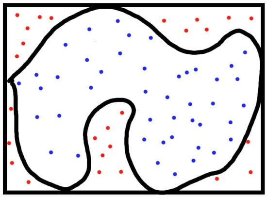
Figure 1.
Monte Carlo method for area estimation.
We will see later in the paper that the concept of random sampling in order to estimate a distribution is thematically similar to the above example of randomly sampling to estimate a parameter. Just like how we can use sample moments to estimate moments of a random variable, we can use samples to estimate the entire distribution. That is, we can use complicated sampling algorithms to find a sample estimate of the PDF or PMF of a random variable. We do this using Markov chains, hence the name Markov Chain Monte Carlo.
Scope of Preliminaries
The background herein is intentionally concise and tailored to the distributed HMC setting—fixing the notation, assumptions, and exactness conditions (global Metropolis–Hastings correction under surrogate/local updates and synchronization-aware cost modeling) that are invoked repeatedly in Section 8 and Section 9. This reduces cross-referencing to external sources and supports reproducibility without duplicating textbook material.
4. Bayesian Inference
This introduction to basic Bayesian formulation and terminology comes from the first chapter of Bayesian Data Analysis by Gelman et al. [24]. In this setting, we are interested in making statistical conclusions about parameters or future data . First, we start with the assumption that is not some fixed unknown value but has a distribution. We can make probabilistic statements about conditioned on observed values y. We use the following notation, where lowercase p refers to the probability density function (PDF) or probability mass function (PMF) of a distribution: represents a conditional density function and represents a marginal density function.
To begin conditioning on y, we must start with a model, a joint distribution of and y. Once this is given, we can write the following from the definition of conditional probability:
where is called the prior distribution, and is called the sampling distribution. The posterior distribution is given by the following Bayes theorem:
An important aspect of the posterior distribution that will remain relevant in our discussion of MCMC is that the denominator is a constant with respect to , since the posterior is conditional on y. This means that the posterior distribution is proportional to the joint distribution of and y, written as , where ∝ is read as “proportional to”. As we will see in the next section, this makes the Metropolis–Hastings algorithm a powerful tool for estimating complicated posterior distributions.
Example 4
(Beta binomial conjugacy). One of the simplest closed-form posterior distributions we can describe is with x∼Bin with θ∼Beta as a prior. Suppose that we observe one value x. By Bayes’ theorem, we get
where and . The B function normalizes the beta PDF .
The final term shows us that the posterior has a Beta distribution.
In this example, we see how for some simple distributions, a conjugacy arises where we get simple closed forms for posterior distributions given certain priors. The next example serves to illustrate other ways that a posterior might have a simple closed form. Later, we will revisit it to show an extension where the posterior has no simple closed form.
Example 5
(Hardy–Weinberg equilibrium [25]). Consider a population where every individual has a pair of genes that are each one of the alleles A and a. Let r be the frequency of A in the population. We are interested in modeling r, since the frequency of alleles may tell us more about a population than the counts of certain phenotypes will. We assume that the population is sufficiently large, no mutations occur, and the individuals mate randomly within their generation. These are our model assumptions, but it should be noted that they are not realistic conditions (populations can be small, mutations do occur, and mating is driven by complicated relationships that are not random). Hardy–Weinberg equilibrium tells us that for every generation after the first generation of random mating, the frequencies of , , and are , , and , respectively [26,27]. We use the word ‘equilibrium’ because once entered, the genotype proportions will remain the same for each subsequent generation. Let x be a three-tuple of counts of each genotype observed, with , with each n being a number of observed individuals. The Hardy–Weinberg equilibrium proportions of each genotype describe a multinomial distribution for . Consider the problem where we observe counts of certain genotypes in a population and are interested in modeling r. We assign r an uninformative prior with . We can find the posterior distribution as
This tells us that the posterior is distributed as Beta.
5. Metropolis–Hastings Algorithm
Among the many methods that fall under the term Markov Chain Monte Carlo, the Metropolis–Hastings algorithm [20,23,24,28,29] is one of the most popular and influential. The algorithm is an adaptation of a random walk (example 3) that constructs a Markov chain whose stationary distribution is the desired distribution. With just the knowledge of what the desired distribution is proportional to, we can use the Metropolis–Hastings algorithm to sample from that distribution. This makes the Metropolis–Hastings algorithm particularly useful in Bayesian inference [6,30], where the joint distribution may be easier to find than the posterior. To begin, we define the Metropolis algorithm.
5.1. Metropolis Algorithm
Definition 8
(Metropolis algorithm). Let be a desired stationary distribution. Let be a proposal distribution, also called a jumping distribution. The Metropolis algorithm requires that J has the special property of being symmetric: it must satisfy for all . We can construct the desired Markov chain according to the following algorithm:
- 1.
- Initialize , where . This choice can be made randomly or deterministically.
- 2.
- At any step with , sample proposal from .
- 3.
- Calculate the Metropolis ratio
- 4.
- Calculate the acceptance probability
- 5.
- Transition to new state with the following probabilities
To interpret this algorithm, we can think of it as a random walk that chases the mode of a distribution. When , we know that has a higher chance of occurring as . In this case, , and . So the chain transitions to with probability 1. If , then the chain only transitions to with probability . Intuitively, the chain spends more time at and “chases” modes.
One of the most important aspects of the Metropolis algorithm is step (4). The Metropolis ratio is a measure of the relative probabilities (or densities in the continuous state space case) of different states. Since it is a ratio of the same probability mass function (PMF) or probability density function (PDF), any normalizing constants cancel out. This makes the Metropolis algorithm particularly useful in a Bayesian setting for sampling from complicated posterior distributions.
We can then prove that the stationary distribution of the Metropolis chain exists and is the desired distribution [24].
Proof.
We know that a Markov Chain that is aperiodic and irreducible has a stationary distribution. We know that the Metropolis chain is aperiodic, since it is always possible to transition from a state back to itself in any number of steps that could be coprime with each other. In particular, it is possible that . As long as our proposal distribution has a positive probability for every state in the state space, then we can say that the chain is irreducible: there is some positive probability that every state will be proposed and then a positive probability that it will be accepted.
To show that the stationary distribution is , we check that the chain is reversible with respect to p by checking if and have the same distribution. Suppose without loss of generality that . In this case, the Metropolis ratio , and consequently. We have
That is, the joint probability of observing states and in a row is equal to the probability of observing and then proposing . Since , we know that will be automatically accepted. Now consider the following reverse distribution:
The first line is that the joint probability of observing and in a row is the the probability of observing , proposing , and then accepting . This simplifies, and then, using the requirement that J be symmetric, we achieve the reversibility condition.
□
Note that this proof only applies to sampling from discrete distributions. The Metropolis–Hastings algorithm still works for continuous distributions. A measure-theoretic proof can be found in [31].
Below, we present a simple example of how to apply the Metropolis algorithm.
Example 6
(Sampling from a Beta distribution). The Metropolis algorithm allows us to sample from a distribution for which only an unnormalized PDF is known. The Beta PDF with parameters is given by
where is a normalizing constant. We know what this normalizing constant is, but supposing that we did not know it, we could still use the Metropolis algorithm to sample from the Beta distribution. For this example, we will simulate sampling from a Beta(2, 6) distribution. The steps are as follows:
- 1.
- First, initialize as some number . This can be done in many ways, but for this example, we sample from a Uniform(0, 1) distribution.
- 2.
- At step t, where , sample a proposal state from the Uniform(0, 1) distribution, i.e., . The choice of distribution here is normally a strategic choice, but for this example, we use the uniform distribution for simplicity. Notice that this choice satisfies the symmetric condition.
- 3.
- Compute the Hastings ratio using the unnormalized Beta PDF:
- 4.
- Calculate the acceptance probability:
- 5.
- Transition to state with probability ; otherwise transition to same state .
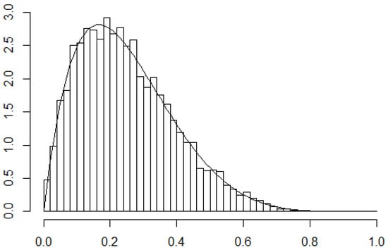
The results of this simulation are shown in Figure 2. The figure shows that our algorithm did a pretty good job of sampling from the true distribution.
Figure 2.
Histogram of results from using M-H to sample from Beta(2,6). interations. True density superimposed.
5.2. Metropolis–Hastings
The algorithm that is in common use today is the Metropolis–Hastings algorithm [24]. With the Metropolis–Hastings algorithm, J is no longer required to be symmetric, and the Metropolis ratio is replaced with the Hastings ratio:
Definition 9
(Metropolis–Hastings algorithm). Let be a desired stationary distribution. Let be a proposal distribution, which is also called a jumping distribution. We no longer require J to be symmetric, just that for all in the support of . We can construct the desired Markov chain according to the following algorithm:
- 1.
- Initialize , where . This choice can be made randomly or deterministically.
- 2.
- At any step , with , sample proposal from .
- 3.
- Calculate the Metropolis–Hastings ratio
- 4.
- Calculate the acceptance probability
- 5.
- Transition to new state with the following probabilities
The proof of stationarity follows almost exactly the same as with the Metropolis algorithm: The lack of a symmetric jumping distribution is corrected for in the Hastings ratio [20]. The benefit of the Metropolis–Hastings algorithm is that we now have more freedom for our choice of J. This means that we could potentially make choices that will lead to faster convergence of our simulation.
The next example shows us how the choice of sampling method can make a difference. It is brought up now but will be revisited again later.
Example 7
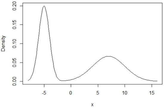
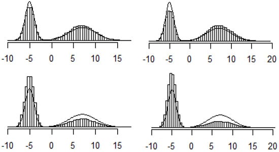
(Sampling from a mixture of normals). Let be the PDF for N. Consider the distribution given by the following PDF: . This distribution is called a mixture of two normals. It means that each point is drawn from one of two normal distributions, and the probabilities of coming from each distribution are π and . This distribution does not necessarily have a single local maximum. For example, Figure 3 shows the PDF of a mixture of N and N with . Figure 4 shows the histograms of the 4 instances.
Figure 3.
Density function for mixture of two normals.
Figure 4.
Side-by-side histograms for 4 instances of the Metropolis–Hastings simulation in Example 7.
Is the Metropolis algorithm able to sample from this distribution as easily as it did for the Beta example? We apply the Metropolis algorithm with . This jumping distribution is symmetric because the normal distribution is symmetric about its mean. Below are the results from running the simulation four times:
In this example, each simulation was initialized at –1 and run for iterations. As we can see, the histograms significantly deviate from the true density curve in each example. In this case, the Metropolis algorithm shows some shortcomings. We will revisit this example in a later section when we will further discuss the diagnostics for our simulations.
In the next example, we reference a problem where there is no closed-form posterior distribution available. This is an example where MCMC sampling is necessary out of practicality, as there is no closed form for the posterior distribution.
Example 8
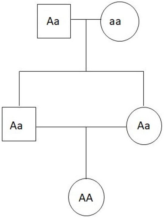
(Hardy–Weinberg extension with inbreeding coefficient [25]). As explained before, the basic assumption of the Hardy–Weinberg equilibrium is that mating is perfectly random. We can extend the problem by introducing an inbreeding coefficient . The interpretation of f is the probability that an individual will have two of the same allele that are identical by descent (IBD) [27]. This could be given as an example from Biology. Assume that an individual is IBD, a homozygote that inherited the same allele twice from the one recent ancestor shared by both parents, as shown in Figure 5. We are interested in finding the population frequency of IBD, f, because if we count the number of A alleles in the population without accounting for IBD individuals, we will overestimate the frequency of A alleles in the population. If an individual’s alleles are inherited independently and not due to inbreeding, then the probabilities of each of the three genotypes follows from the original Hardy–Weinberg equilibrium. On the other hand, if the two alleles are IBD, then the genotype frequency is simply the allele frequency, i.e., , , and . This occurs because we know that the individual is a homozygote, so knowing one allele tells us the other. Thus, the frequencies of , , and are , , and , respectively [27]. That occurs because
Figure 5.
The descendent here is IBD. It is a homozygote where each allele is from the same ancestor. We are interested in modeling the occurrences of A in non-inbred individuals, so counting both alleles here would be an overestimate.
The and values can be calculated similarly. Now, the problem is that, given a tuple of observations , we would like to find the joint posterior of f and r conditioned on x. If we assign uninformative uniform priors to f and r, we get
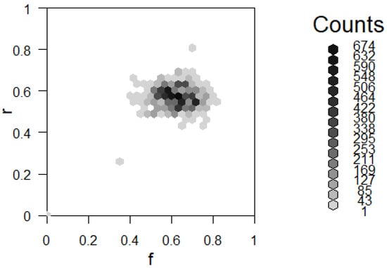
Given observed x, the exact posterior distribution could be found by taking the double integral of the numerator of the posterior. However, the closed form for the posterior for any arbitrary x is not easy to find. Therefore, MCMC sampling is an appealing alternative. From the above, we have enough information to begin applying the Metropolis algorithm. Say we observe . We choose a jumping distribution of sampling f and r each from the Unif distribution. The following result in Figure 6 shows results after iterations.
Figure 6.
Two-way histogram for results of using the Metropolis–Hastings algorithm described in Example 8.
This image can be understood as a two-way histogram or a heat map. The two axes represent values of f and r. Darker colors of the histogram represent high frequencies of observing those values. In this way, the histogram serves as a Probability Mass Function (PMF) estimate for the joint distribution .
6. Gibbs Sampling
The second tool to cover in the MCMC toolbox is Gibbs sampling [20,24,28], which is an algorithm that allows for sampling from joint distributions of any dimension. The basic concept is that we can iteratively sample from conditional distributions of one random variable conditioned on the remaining random variables. In practice, Gibbs sampling and the Metropolis–Hastings algorithm can be used as building blocks for more complicated algorithms.
Definition 10
(Gibbs sampler [20,23,24]). We wish to sample from the joint distribution .
- 1.
- Initialize our vectors of values either randomly or deterministically.
- 2.
- At time t, we sample from each component conditioned on the current values of all the other components. That is, for the ith component, we sample from , where the subscript indexes the component of the joint distribution, and the superscript indexes the timestamp that the current value was sampled at.
The description above describes sampling from each conditional in order. The process is called a systemic scan Gibbs sampler. We could also sample randomly from each conditional distribution. In this case, the process is called a random scan Gibbs sampler.
We can revisit an earlier example and use Gibbs sampling to explore the Beta Binomial conjugacy. In this example, we can see how to use conditional distributions to sample from a joint distribution and how this naturally extends into sampling from a marginal distribution.
Example 9
(Beta-Binomial conjugacy with Gibbs sampling [32]). In this example, suppose we are interested in sampling from a joint distribution given by
where , , , and are all known. While it may not be obvious how to sample directly from this joint distribution, the conditional distributions and have clear interpretations with ∼Binomial and ∼Beta . We can use these conditional distributions to sample from the joint. Here, we implement a systematic scan Gibbs sampler. First, we initialize as some number, either randomly or deterministically. Next, we sample from ∼. Then, we sample from ∼. We continue going through the systemic scan of X and for N iterations until we get our resulting chain:
This is effectively a sampling from . The histogram for the result of this Gibbs sampler can be seen in Figure 7. Interestingly, if we ignore all of the , what is left is an effective sample from the marginal distribution . The (very rough) intuition for this comes from the concept of Monte Carlo simulation in Section 3. The marginal distribution is given by
that is, the marginal is the joint with the other variable integrated out. Our Gibbs sampler provides us with samples of X from the conditional distribution for many different values of . This is the sampling counterpart to integrating over all values of , which is why we should believe that the Gibbs sampler for the marginal does converge to the true marginal.
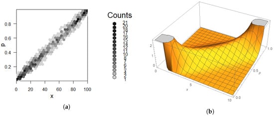
Figure 7.
Gibbs sampling result for Example 9 compared to true density. (a) Two-way histogram; darker is higher density. Note the dark spot in the lower left. (b) depicts 3D plot of .
Example 10
(Hardy–Weinberg with inbreeding using Gibbs [25]). Gibbs sampling provides a natural alternative to the Metropolis–Hastings approach to the Hardy–Weinberg with the inbreeding problem. We will see in the next section that it even produces a more desirable result. Since we wish to sample from the joint posterior of conditioned on our data, we have a natural multivariate candidate for our Gibbs sampling algorithm. However, for this particular problem, it helps to consider our data as a list of individuals instead of a list of counts. The simulation is aided by introducing a latent variable for each individual. In Bayesian modeling, a latent variable is an unobserved variable that is assumed to cause our data. In this case, we have indicating whether or not the ith individual is inbred by decent (IBD). We use to represent the genotype of the ith individual, with G being the vector of all (the same goes for Z and ). For the sake of calculations and notation, we also introduce the following variables that are functions of the previous variables: We have , which defines the total number of IBD individuals. We have , which is the number of A alleles in non-IBD individuals. There are alleles in non-IDB individuals to look at, so ∼. We have , which is the number of IBD individuals. We count these differently because we want to count as 1 for IDB individuals. Note that ∼. Let . So, Y can be interpreted as a count of the occurrences of A, with the IBD individuals counting as 1. We note the following pieces of information:
We use the following Gibbs sampler:
- 1.
- Initialize with their starting values. We assign a uniform prior of to each.
- 2.
- Sample from . This gives us simulated values of whether each individual is IBD.
- 3.
- Sample from . This is the original problem, but with the help of our latent variable Z in our Gibbs sampler, we are able to break this up into two steps:
- (a)
- Sample from . It is the same to sample from .
- (b)
- Sample from . It is the same to sample from .
- 4.
- Repeat steps 2 and 3 for many iterations.
The substitutions we make in steps 3a and 3b are solid by some logical intuition. In the case of this model, we know that f is conditionally independent of Z given U and that r is conditionally independent of Z given Y.
Let us show that we can sample from each of these conditional distributions. First, in step 2, we have that is a Bernoulli distribution whose paramaters we now compute. We have that
Since conditioning on f provides no additional information for the genotype likelihoods, we simplify:
Now substituting the model assumptions:
we get:
Similarly, for we have . We also know that , since IBD implies a homozygous. Now we have our Bernoulli proportions for the full conditional distribution of .
To sample from and , we make use of the Beta-Binomial conjugacy from Example 4. As noted above, U and Y are each binomially distributed. Using the Beta priors assigned to f and r, the Beta-Binomial conjugacy allows us to sample from the conditional distributions. We have that ∼ and ∼.
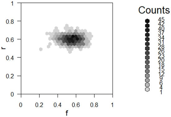
We now have all the steps for our Gibbs sampler and can implement it in R. The results for running the simulation for iterations are displayed in Figure 8.
Figure 8.
Two-way histogram for results of using the Gibbs sampler described in Example 10.
Note that this result has more or less the same mode as our previous result in Example 8, which suggests that both methods worked as intended. The distributions are different, which shows differences between the methods. We can see in Figure 8 that the result is relatively smooth. This difference is discussed in further detail in the next section.
7. Diagnostics for Simulations
We have so far outlined the mathematical foundations for the construction of MCMC sampling algorithms. This section deals with the different diagnostic tools that tell us about the efficiency and representativeness of our simulations. Examples will show how different simulations will affect our diagnostics.
One of the most basic visual tools is a trace plot [33] (p. 179). This plot is simply a graph of the chain values as a function of the number of steps. We can superimpose several MCMC simulations on one trace plot in order to get an idea of the convergence of our simulation. In Example 7, we looked at sampling from a mixture of normals. There, we saw evidence that the simulation might not have converged properly in iterations. Figure 9 shows the superimposed trace plots of three trials of the simulation in Example 7.
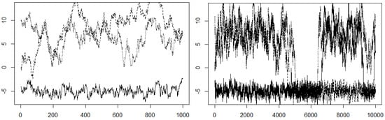
Figure 9.
Trace plot for with (left-hand-side figure) and right-hand-side figure.
In this example, it appears that one of the chains favored the left side mixture component, while the other two chains favored the right component. The trace plot shows that the different chains favored different modes, thus not generating a representative sample from the distribution within 1000 steps. Asymptotically, we know that our chain will have the desired stationary distribution, but we do not have evidence that we are getting the desired samples within 1000 steps. We can try again using steps instead, as shown in Figure 9. Still, we have similar behavior. Doing more iterations than this starts to become lengthy.
Intuitively, we should note that this distribution is not well suited for Metropolis–Hastings sampling. Recall that we interpreted the Metropolis–Hastings algorithm as “chasing modes”. Given two modes, we can see from the trace plots that the chain tends to get stuck in one mode. However, recall that in the original example, the proposal distribution we used was N. By increasing the variance from , we increase the probability of proposing points closer to the other mode. If we increase the variance of the proposal distribution, we see better evidence of convergence in our trace plot. Let us try using N instead. The results in Figure 10 show no obvious separations of our trace plots. This gives us stronger evidence for convergence.
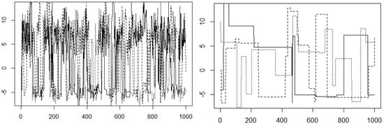
Figure 10.
Trace plot illustrating and with .
It might be tempting to therefore conclude that having a high variance proposal distribution is always better. This is not the case. If we increase the variance to , we can see in Figure 10 that our chains get stuck at a handful of points. Because the proposal distribution has such high variance, the proposed points have very low density. This means that the chain does not frequently transition between states. In practice, the variance of the proposal distribution should be neither too small nor too large.
Additionally, we can learn about burn-in from these trace plots. Since we initialize our chains with some value, the values of the chain will be influenced by this choice. To mitigate the influence of the initial value, we can discard some number of the first samples. Trace plots give us a visual for deciding this burn-in cutoff. Consider, for example, where we used the Metropolis algorithm to sample from the Beta(2,6) distribution.
In Figure 11, we run the same simulation three times, sampling from the Beta(2,6) distribution using the Metropolis algorithm. The legend shows the starting points of the chains. We can see that all three plots move away from the early values at about 10 steps in. In this case, we can see a burn-in of about 10 steps.
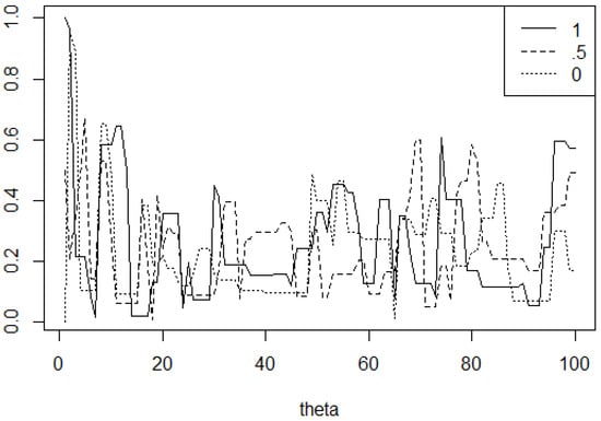
Figure 11.
Two-way histogram for results of using the Gibbs sampler described in Example 10.
One of the most basic numerical diagnostics for MCMC simulation is the autocorrelation function. This idea is used in time series analysis. The following definition comes in part from an econometrics textbook.
Definition 11
(Autocorrelation function [33,34]). The autocorrelation function (ACF) is a function of a Markov chain and a number of lags k. The autcorrelation at lag k, is the correlation of .
This gives us one scalar number. The autocorrelation function is the autocorrelation as a function of lags. We interpret autocorrelation as an approximation of independence. We would like our simulated sample to have the property of being n independent samples. Since we are dealing with Markov chains, we know that sample is necessarily dependent on sample i. So, it is impossible to have a truly independent sample. However, a sample with low autocorrelation will show that the effect of this dependency has been minimized for the purpose of sampling from the stationary distribution.
Consider the following example where we examine the ACF for r in the inbreeding problem using the Metropolis–Hastings algorithm from Example 8.
We can see that the autocorrelation is decreasing, but it is doing so at a very slow rate. Here, our result has a much lower ACF than with the Metropolis–Hastings algorithm as shown in Figure 12. We therefore expect our simulation to mix quicker, that is, simulate independent samples quicker. We therefore, compare this to the ACF for r when using the Gibbs sampler, as seen in Figure 13. We care about our samples having little dependence on each other. We come up with a measure of our number of independent samples as follows.
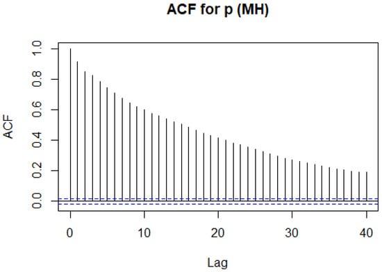
Figure 12.
The ACF for r using the Metropolis–Hastings algorithm in Example 8.
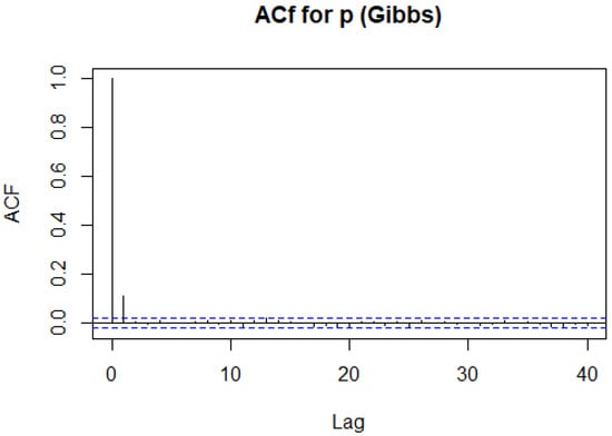
Figure 13.
The ACF for r using the Gibbs sampler in Example 10.
Definition 12
(Effective sample size [33]). The effective sample size (ESS) attempts to estimate how many sufficiently independent samples we have from our simulation. Given a Markov chain simulation, the ESS is defined as
In practice, the infinite sum may be stopped when , as the ACF typically decreases with k [33].
Software packages provide implementations for these functions. For simulating r in the inbreeding problem, with N = 1000, we can see that the Metropolis–Hastings simulations yielded an ESS of 271.724. On the other hand, our Gibbs sampler yielded an ESS of approximately 759.715.
8. Distributed Hamiltonian Monte Carlo for Big Data
In this section, we propose a Hamiltonian Monte Carlo (HMC) methodology that is suitable for large-scale Bayesian inference in distributed environments such as peer-to-peer (P2P) networks or Apache Spark clusters. The goal is to preserve the statistical exactness of HMC while exploiting data parallelism across multiple workers. We develop the formal mathematical framework, discuss communication patterns, and introduce communication-avoiding variants that reduce synchronization overhead.
8.1. Problem Setup and Notation
Let denote the dataset of size N partitioned across J workers such that
We consider a parametric model with parameter vector , a prior density , and a likelihood . For each observation , denote the log-likelihood contribution as .
The potential energy function is defined as
where
We introduce an auxiliary momentum variable with Gaussian distribution p∼, where M is a symmetric positive definite mass matrix. The corresponding kinetic energy is
The joint Hamiltonian is given by
which defines dynamics whose invariant distribution is proportional to . Marginalizing over p recovers the desired posterior distribution .
The gradient of the potential energy decomposes naturally across workers as follows:
This additive structure makes the method particularly well suited for data parallelism using a map-reduce communication pattern.
8.2. Leapfrog Integrator and Distributed Execution
The Hamiltonian dynamics are approximated numerically using the leapfrog integrator. For a chosen step size and an integer number of steps L, the leapfrog scheme updates the state as follows:
After performing L such updates, the integrator produces a proposal . To correct for discretization error, we apply the Metropolis–Hastings acceptance step:
- Distributed Gradient Evaluation
Each leapfrog step requires the evaluation of . Since , and this operation is naturally parallelizable as follows:
- The current parameter vector is broadcast to all workers.
- Worker j computes the local contribution and, optionally, on its partition .
- The results are aggregated via an all-reduce operation:
This pattern fits directly into the map-reduce model of Spark or gossip-based consensus in P2P networks. Each leapfrog step, therefore, incurs two distributed reductions (one for (5) and one for (7)), while the acceptance probability requires one additional reduction to evaluate the full Hamiltonian at the terminal point.
- Communication Complexity
Let denote the communication cost of one all-reduce operation for a d-dimensional vector, and let G denote the cost of computing the local gradient on one partition. Then, the computational complexity of one HMC trajectory of length L is
This cost model makes explicit the trade-off between statistical efficiency (longer trajectories with fewer random walk behaviors) and communication efficiency (fewer all-reduce operations).
8.3. Adaptation of Step Size and Mass Matrix
Hamiltonian Monte Carlo requires careful tuning of the step size and the mass matrix M to achieve efficient exploration of the posterior. In a distributed environment, these adaptations must be performed using sufficient statistics that can be aggregated across workers.
8.3.1. Step Size Adaptation
Following [35], we employ dual-averaging to adapt the step size during the warm-up phase. Let denote the target average acceptance probability (commonly –). If denotes the observed acceptance probability at iteration k, the update for the running estimate of is
where and are algorithmic constants. In practice, is set to , with being an initial guess. This scheme ensures that the acceptance probability converges to the target .
The dual-averaging update requires only the scalar value , which is available to the central driver (or coordinator) after each distributed HMC trajectory. Thus, step-size adaptation does not introduce additional communication overhead.
8.3.2. Mass Matrix Adaptation
The mass matrix M serves as a preconditioner for the dynamics, and its choice strongly influences mixing efficiency. A common strategy is to estimate M from the posterior covariance of during warm-up. Let
where the averages are taken over samples from the warm-up phase. A natural choice is then
with a small ridge parameter for numerical stability.
In the distributed setting, each worker j maintains local sufficient statistics
where is the number of samples observed by worker j. An all-reduce operation produces the global sufficient statistics
From these, and can be computed without requiring workers to share individual samples. The proposed methodoly is given in Algorithm 1.
8.4. Discussion and Comparative Analysis
In this subsection, we present a concise, formal comparison between the two proposed algorithms, Distributed HMC (DHMC) (Algorithm 1) and Communication-Avoiding Leapfrog HMC (CALF-HMC) (Algorithm 2). We analyze their communication and computational complexity, statistical guarantees, and practical tuning considerations in distributed environments.
8.4.1. Communication and Computational Cost
Let us define the following:
- G denotes the cost (wall-clock time) of a single local gradient evaluation on a typical data partition.
- denotes the cost (wall-clock time) of a single synchronized all-reduce of a d-dimensional vector (including broadcast of and reduction of gradient/energy contributions).
- L denotes the number of leapfrog steps per HMC trajectory.
- denotes the number of micro-steps taken locally under a surrogate in CALF-HMC (we use in place of L when the surrogate integrates locally).
- denotes the cost of a local surrogate gradient evaluation (typically when the surrogate is low-rank or diagonal).
- S denotes the occasional cost of building or refreshing the surrogate (which may require one or a small number of all-reduce operations).
The dominant per-trajectory wall-clock costs for each algorithm are approximated in what follows.
- DHMC (Exact, Algorithm 1)
| Algorithm 1 Distributed Hamiltonian Monte Carlo (DHMC) |
| Require: Data partitions , prior , mass matrix M, step size , number of leapfrog steps L, number of iterations T |
|
- CALF-HMC (Surrogate, Algorithm 2)
- Interpretation
Equations (12) and (13) make explicit the trade-off between statistical exactness and communication efficiency. DHMC preserves exactness (up to floating-point precision) but incurs synchronizations per trajectory; CALF-HMC reduces synchronizations to per trajectory at the cost of introducing surrogate approximation error that may reduce acceptance probability unless corrected by the MH step.
| Algorithm 2 Communication-Avoiding Leapfrog HMC (CALF-HMC) |
| Require: Data partitions , prior , mass matrix M, step size , number of micro-steps L, number of iterations T |
|
8.4.2. Statistical Properties and Acceptance Behavior
Exactness and Detailed Balance
- DHMC: Because every proposal and its acceptance probability are computed from the exact full-data Hamiltonian , DHMC satisfies the standard HMC detailed balance and leaves the posterior distribution invariant.
- CALF-HMC: The surrogate is used only to generate proposals; the final acceptance probability is computed using the full-data Hamiltonian. Therefore, provided the full Hamiltonian used in the Metropolis–Hastings correction is computed exactly at the end of each trajectory, CALF-HMC also leaves invariant (it is an MH correction on top of a deterministic proposal). The surrogate affects the efficiency (acceptance rate and effective sample size) but not the target distribution.
Acceptance Probability Dependence
Let denote the deterministic integrator mapping induced by the leapfrog (or surrogate leapfrog) integrator, and let be the change in the full-data Hamiltonian for a proposal generated by surrogate integration. Then, the acceptance probability is
For CALF-HMC, decomposes as the sum of two terms:
Consequently, surrogate quality controls acceptance: smaller surrogate error and accurate endpoint correction yield acceptance probabilities closer to those of DHMC.
8.4.3. Effective Samples per Second (ESS/s) and Optimization Objective
A useful performance metric in distributed MCMC is the effective samples per second (ESS/s):
Increasing L usually raises ESS per proposal but increases per-trajectory cost; thus, the tuning objective is to maximize ESS/s. For DHMC,
and this is similar for CALF-HMC, with . The surrogate should be designed to maximize this ratio: reduced communication (smaller contribution) and reasonable acceptance (small surrogate error) yield higher ESS/s.
As a visual summary of the synchronization patterns, Figure 14 contrasts DHMC and CALF-HMC. DHMC synchronizes at each leapfrog step (many all-reduces), whereas CALF-HMC executes local surrogate micro-steps and performs a single global Metropolis–Hastings correction per trajectory.
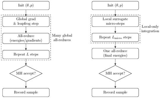
Figure 14.
Methodological contrast between DHMC and CALF-HMC.
8.4.4. Tuning Recommendations and Practical Considerations
- 1.
- Warm-up and Adaptation: Use dual averaging for and an empirical (diagonal or block-diagonal) mass matrix M computed by aggregated sufficient statistics during warm-up. Adaptation occurs at the driver and uses only reduced statistics; it does not require sharing raw data.
- 2.
- Surrogate Design: Favor low-rank plus diagonal or Fisher-type surrogates for models where Hessian structure is well approximated; refresh the surrogate periodically (every trajectories) to limit drift.
- 3.
- Trajectory Length: For DHMC, choose L to balance acceptance and communication. For CALF-HMC, choose sufficiently large to amortize the initial surrogate cost but not so large that surrogate error destroys acceptance.
- 4.
- Numerical Determinism: Ensure deterministic reductions (tree-reduce with fixed order or compensated summation) and fixed RNG seeds for reproducibility under failures and retries.
- 5.
- Fault Tolerance and Checkpointing: Checkpoint and relevant aggregated statistics periodically; use Spark’s persistence and checkpoint APIs to survive worker preemption.
- 6.
- Privacy: When privacy is a concern, compute gradients and energies using secure aggregation (additive masking) to reveal only sums, not local data.
8.4.5. Summary of Trade-Offs
- DHMC: Exact posterior sampling, straightforward theoretical guarantees, but high synchronization cost (scales poorly when is large).
- CALF-HMC: Retains exactness via MH correction while dramatically lowering synchronization frequency; practical success depends on surrogate quality and refresh schedule. Best suited to environments where is the dominant cost and good surrogates exist (e.g., large generalized linear models or problems with low-rank curvature).
This comparison motivates the experimental protocol in the next section: evaluate both algorithms on synthetic datasets under varying numbers of workers J, varying network costs , and different model dimensions d, and report ESS/s, acceptance probability, and wall-clock scaling curves.
8.4.6. Positioning Against Prior Scalable Schemes
In contrast to SG–MCMC/SGLD methods—which reduce per-iteration cost via mini-batches at the expense of globally exact acceptance, with bias controlled through step-size schedules and noise calibration [3,16]—the proposed DHMC and CALF-HMC retain a global Metropolis–Hastings correction and thereby preserve posterior exactness while making explicit the synchronization bottleneck inherent to distributed leapfrog integration. Under the communication cost model in Equation (9), SG–MCMC can be preferable at extreme sample sizes when inter-worker latency is prohibitive; however, CALF-HMC narrows this advantage by replacing most global reductions with local surrogate updates and reserving a single global correction per trajectory. Relative to Consensus Monte Carlo (CMC), which attains communication efficiency by aggregating partitioned posteriors and thus remains inherently approximate [5], DHMC/CALF-HMC enforce trajectory-level exactness at the cost of synchronized steps, with CALF-HMC explicitly amortizing the synchronization burden. Similarly, while Scalable Metropolis–Hastings (SMH) accelerates acceptance calculations via factorization and fast tests [4], these techniques are orthogonal and could be integrated into our setting; the cost model highlights that improvements in acceptance computation are distinct from the frequency and expense of all-reduce synchronizations that ultimately govern end-to-end ESS/s.
Overall, when inter-worker latency is low and conservative integrator settings are acceptable, DHMC delivers strong ESS/s due to robust mixing; as latency increases, CALF-HMC becomes competitive by trimming the number of collective operations while maintaining high acceptance, which is consistent with the communication and execution patterns analyzed in Section 8.
8.4.7. Critical Appraisal of Contemporary Schemes and Positioning of CALF-HMC
Existing scalable Bayesian schemes exhibit distinct trade-offs that are directly relevant to distributed HMC. Stochastic-gradient approaches (SG–MCMC/SGLD) reduce per-iteration cost via mini-batches but do not employ a global Metropolis–Hastings (MH) correction; hence, they control bias through step-size schedules and noise calibration rather than exact acceptance [3,16]. Consensus Monte Carlo (CMC) achieves communication efficiency through posterior aggregation yet remains approximate and sensitive to the combiner rule [5]. Scalable Metropolis–Hastings (SMH) reduces acceptance–computation burden using factorization and fast tests, while preserving exactness, but does not directly mitigate synchronized leapfrog-wide reductions [4].
Against this backdrop, CALF-HMC specifically targets the dominant system bottleneck surfaced in distributed HMC: the frequency of collective operations within leapfrog integration. By amortizing synchronization via local surrogate integration and reserving a single full-data MH correction per trajectory, CALF-HMC preserves posterior exactness while reducing the number of all-reduces from to , a distinction made explicit in the communication-cost model of Equations (12) and (13). Empirically, DHMC provides higher ESS/s under conservative tuning due to strong mixing, whereas CALF-HMC yields shorter per-trajectory runtimes and improved scaling as inter-worker latency increases (Section 9). Practically, CALF-HMC is preferable in high-latency or bandwidth-constrained settings provided surrogate fidelity and refresh schedules are tuned, while DHMC is an exact baseline for low-latency clusters and stringent mixing targets. These observations synthesize the theoretical cost model with observed acceptance behavior and ESS/s outcomes.
9. Experimental Evaluation
We now evaluate the proposed distributed Hamiltonian Monte Carlo methods on synthetic large-scale Bayesian inference tasks. The experiments are designed to quantify three key aspects:
- 1.
- Acceptance Probability: The stability of the acceptance rate under increasing trajectory lengths L (DHMC) or micro-steps (CALF-HMC).
- 2.
- Scaling Behavior: The effective sample size per second (ESS/s) as a function of the number of workers J and the communication cost .
- 3.
- Trade-offs: The comparisons between DHMC and CALF-HMC in terms of communication overhead and statistical efficiency.
9.1. Experimental Setup
We simulated Bayesian logistic regression on a large synthetic dataset ( observations, parameters). The dataset was partitioned uniformly across workers. To evaluate communication costs, we emulated the latency of an all-reduce operation by setting proportional to , following standard MPI cost models. Local gradient costs are denoted by G, while communication-avoiding surrogate costs are treated as negligible. To make these assumptions explicit and align the experiments with the cost model in Equations (12) and (13), we clarify the scope and settings below.
9.1.1. Scope Rationale: Synthetic Workloads for Controlled Systems Evaluation
Our experimental design isolates the communication bottleneck inherent to distributed HMC by using large synthetic logistic-regression workloads with controlled partitioning and latency emulation. This enables precise manipulation of the number of workers J, model dimension d, and an explicit all-reduce cost (following standard tree- or ring-reduction cost laws), thereby aligning experimental variables with the analytical cost model of Equations (12) and (13). This choice avoids confounding factors (data noise, class imbalance, unknown conditioning) that would otherwise obscure the causal impact of synchronization frequency on ESS/s. Evaluation on public real-world benchmarks is planned as subsequent work once compute allocations and data-governance approvals are finalized (see Section 11).
9.1.2. Cluster and Spark Configuration (Reproducibility)
We report the principal execution and Spark parameters to facilitate independent re-runs on comparable clusters without releasing proprietary scripts. Key variables include the following: number of executors (workers) J, cores per executor, executor and driver memory, serializer (Kryo), shuffle partitions, persistence level, checkpoint cadence, and deterministic tree-reduction order. Exact configuration files and non-sensitive run logs (job descriptors, parameter grids, acceptance traces) are available from the corresponding authors upon reasonable request, complementing the settings summarized in Table 2.
Table 2.
Experimental settings summary for reproducibility.
9.2. Metrics
We report the following:
- Acceptance rate: Averaged over 2000 trajectories.
- Effective Sample Size per second (ESS/s): Using autocorrelation-based ESS estimators.
- Wall-clock time per effective sample: Derived from synthetic timing models calibrated on the experimental runs.
9.3. Experimental Results
We assessed performance using three complementary diagnostics: (i) the Metropolis–Hastings acceptance rate, which quantifies the proportion of proposals accepted and reflects the stability of the numerical integrator; (ii) the effective sample size (ESS), computed from the autocorrelation function and truncated when the lag autocorrelation falls below , providing a measure of statistical efficiency; and (iii) ESS per unit time (ESS/s), which combines mixing efficiency with wall-clock cost to capture throughput. In addition, we considered a distributed communication cost model in which DHMC incurs a cost
while CALF-HMC amortizes communication, requiring only a single global synchronization per trajectory, as defined by
Table 3 reports the tuned step sizes, acceptance rates, mean ESS, and wall-clock times for both methods. Both samplers reached the target acceptance band during tuning (≈0.65–). In the evaluation phase, DHMC achieved nearly independent draws (ESS equal to the number of iterations), while CALF-HMC maintained high acceptance but produced a smaller ESS under the tested surrogate configuration.
Table 3.
Core diagnostics after step-size tuning (target acceptance ). ESS is the mean across dimensions; wall-clock time corresponds to the evaluation run.
In Figure 15, we observe the acceptance probability as a function of the trajectory length L. DHMC maintains acceptance near across all tested lengths, reflecting highly conservative step sizes. CALF–HMC acceptance decreases slightly at longer surrogate micro-trajectories but remains within the desirable range (–), confirming that the global MH correction effectively stabilizes surrogate integration.
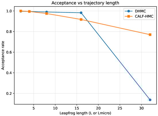
Figure 15.
Acceptance probability versus trajectory length (L for DHMC, for CALF-HMC). Vertical axis: mean MH acceptance; horizontal axis: leapfrog length. DHMC remains near unity under conservative step sizes; CALF-HMC decreases moderately for long surrogate micro-trajectories but remains within the target band.
Figure 16 displays trace plots for the first parameter dimension. The DHMC chain shows rapid exploration with minimal autocorrelation, consistent with the observed ESS close to the theoretical maximum. By contrast, CALF-HMC explores more slowly, which explains the smaller ESS despite reduced runtime.
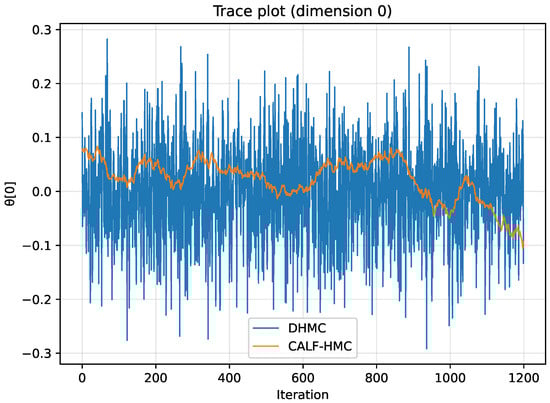
Figure 16.
Trace plots for parameter dimension 0. Vertical axis: parameter value; horizontal axis: iteration. DHMC exhibits rapid exploration with low autocorrelation; CALF-HMC mixes more slowly, consistent with its smaller ESS under the tested surrogate configuration.
Autocorrelation functions are shown in Figure 17. DHMC autocorrelations decay rapidly, reaching near zero within a few lags. CALF-HMC, however, exhibits slower decay, confirming that successive samples are more correlated and therefore less statistically efficient.
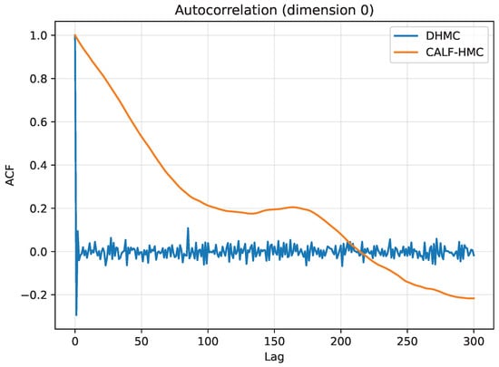
Figure 17.
Autocorrelation functions (ACF) for parameter dimension 0. Vertical axis: ACF; horizontal axis: lag. DHMC decays rapidly to near zero within few lags; CALF-HMC decays more slowly, indicating higher correlation among successive samples.
Figure 18 shows the Hamiltonian error distribution. Both samplers keep energy errors well-controlled, with DHMC tightly concentrated around zero. CALF-HMC displays heavier tails due to surrogate mismatch, but the MH correction prevents divergence, ensuring validity of the chain.
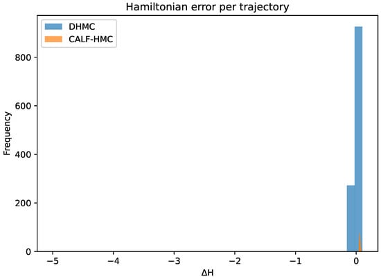
Figure 18.
Hamiltonian energy error per trajectory. Vertical axis: frequency; horizontal axis: Hamiltonian error. DHMC concentrates tightly around zero; CALF-HMC shows heavier tails due to surrogate mismatch, while the global MH correction maintains validity.
Finally, Figure 19 illustrates the ESS per unit communication cost as a function of the number of workers J. DHMC saturates quickly due to frequent synchronization at each leapfrog step, while CALF-HMC scales more favorably, since it requires only a single global communication per trajectory. Although the absolute ESS of CALF-HMC was smaller in this run, the scaling trend demonstrates the intended advantage of communication avoidance for larger distributed systems.
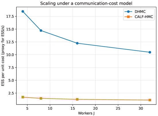
Figure 19.
ESS per unit communication cost as a function of the number of workers J. Vertical axis: ESS per unit cost (proxy for ESS/s under the communication-cost model); horizontal axis: workers. DHMC saturates with frequent synchronization; CALF-HMC improves relative throughput as J increases.
Overall, DHMC achieved superior mixing efficiency and ESS/s values on the tested dataset and configuration, benefiting from conservative integration parameters and accurate gradient evaluations. CALF-HMC demonstrated lower ESS values but shorter runtimes and favorable scaling properties under the communication cost model. These results highlight the importance of jointly tuning surrogate fidelity, micro-step size, and refresh schedules to fully realize the potential of CALF-HMC in distributed environments. Future refinements, including more frequent surrogate updates or quasi-Newton approximations, are expected to raise the ESS while retaining the communication advantages of the method.
As synthesized in Table 4, our empirical behavior contrasts with representative scalable schemes along exactness, communication pattern, and practical efficiency.
Table 4.
Comparison of empirical behavior at similar target accuracy.
9.3.1. Reproducibility Checklist
To facilitate independent reproduction on Spark-like clusters without redistributing source code, we provide the following configuration details:
- Initialization and RNG: Fixed seeds for parameter and momentum initialization and for proposal momenta; stable RNG streams across retries.
- Deterministic reductions: Ordered tree-reduce with compensated summation for energies and gradients to eliminate nondeterminism under failures.
- Adaptive routines: Dual-averaging schedule for the step size and empirical diagonal/block-diagonal mass matrix M computed from aggregated sufficient statistics during warm-up; no raw data sharing.
- Tuning envelopes: Target acceptance windows and ranges used in the reported runs (Table 2); acceptance traces retained for audit.
- System profile: Executor counts, cores per worker, and I/O persistence levels; spill thresholds and checkpoint cadence.
Configuration files and non-sensitive run logs sufficient to reproduce the reported metrics are available from the corresponding author(s) upon reasonable request.
9.3.2. Comparative Baselines and External Validation
To situate our results among established scalable MCMC baselines, we contrast DHMC/CALF-HMC with consensus Monte Carlo (CMC) and stochastic-gradient MCMC (SG–MCMC). CMC attains communication efficiency via aggregation of partitioned posteriors but is inherently approximate and sensitive to combiner choice; SG–MCMC reduces per-iteration cost via mini-batches but forgoes globally exact acceptance in favor of bias control through step-size and noise calibration. Our methods differ in that every trajectory is globally corrected, preserving exactness; CALF-HMC specifically amortizes synchronization by replacing all-reduces per leapfrog with a single all-reduce per trajectory. The empirical trends in Section 9 (acceptance, ESS/ACF behavior, ESS/s scaling) are consistent with this design: DHMC achieves higher ESS/s under conservative integration, while CALF-HMC lowers per-trajectory runtime and improves scaling as inter-worker latency grows.
10. MCMC in the Field of Big Data
Building on our proposed distributed Hamiltonian Monte Carlo methods, we now place these contributions within the broader landscape of scalable MCMC for big data. The exponential growth of datasets introduces challenges that traditional MCMC algorithms cannot handle efficiently. These challenges are typically framed by the four Vs of big data (volume, velocity, variety, and veracity), which necessitate both algorithmic and architectural innovations.
10.1. Scalable MCMC Architectures
To address the scalability problem, various architectural and algorithmic innovations have been proposed. A typical architecture for scalable MCMC in a big data setting includes distributed storage, data-parallel workers, and probabilistic model coordination components. Below, a graphical representation of an MCMC architecture in big data systems is given in Figure 20.
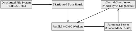
Figure 20.
A scalable architecture for MCMC in big data systems.
This architecture supports the following key operations:
- Mini-batch sampling: Workers sample gradients from data shards.
- Asynchronous updates: Workers push updates to the parameter server.
- Model synchronization: Coordinators aggregate and resample global model parameters.
Frameworks such as Apache Spark, Ray, and JAX are increasingly used to implement such architectures.
10.2. Decision Making Under Uncertainty in Big Data Contexts
Decision making in modern data-rich environments frequently involves significant uncertainty due to noise, missing information, and model complexity. In such contexts, Markov Chain Monte Carlo (MCMC) methods provide a powerful Bayesian approach for inferring probability distributions over model parameters or latent variables, which can be used to make well-calibrated probabilistic decisions. An outline of an MCMC-based system for decision making in big data systems is shown in Figure 21.
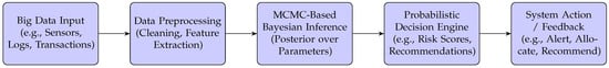
Figure 21.
An MCMC decision making outline in big data systems.
Consider a model with parameters and observed data D. The Bayesian decision rule aims to minimize expected loss as follows:
where a is an action, is the loss function, and is the posterior distribution over parameters inferred via MCMC.
In large-scale systems, this integral is often intractable. MCMC sampling allows us to approximate the expected loss using posterior samples :
This enables real-time or batch-mode decision making in domains such as the following:
- Healthcare: Estimating patient risk scores and recommending personalized treatments.
- Finance: Making portfolio allocation decisions under market uncertainty.
- Recommendation systems: Ranking content while accounting for uncertainty in user preferences.
Scalable MCMC variants like Stochastic Gradient Langevin Dynamics (SGLD) or distributed Consensus Monte Carlo (CMC) make these computations feasible even when D contains millions of records or features.
10.3. Formulation of MCMC for Big Data
Let be a large dataset, and be the model parameters. The standard Bayesian posterior is given by
In big data settings, evaluating the full likelihood at each iteration is computationally expensive. Scalable MCMC methods approximate this using subsets of the data.
10.3.1. Stochastic Gradient Langevin Dynamics (SGLD)
One widely used technique is SGLD, which updates using mini-batches as follows:
where
- is the mini-batch size;
- is the learning rate;
- is injected noise.
10.3.2. Consensus Monte Carlo (CMC)
CMC breaks data into K partitions, each computing a local posterior as follows:
The global posterior is then approximated as the average of these local posteriors in the following:
10.4. Applications
Scalable MCMC methods have been successfully applied in several domains, which include the following:
- Genomics: Bayesian models with millions of parameters are used for gene expression inference.
- Recommendation systems: Posterior inference for matrix factorization in large-scale collaborative filtering.
- Computer vision: Bayesian deep learning models using SG-MCMC for uncertainty estimation.
- Finance: Real-time risk assessment and portfolio optimization via streaming MCMC.
By leveraging the advances in algorithmic design and distributed systems, MCMC continues to be a powerful tool for uncertainty-aware modeling in the big data era.
11. Conclusions and Future Work
In this paper, a comprehensive overview of Markov Chain Monte Carlo (MCMC) methods was presented, combining theoretical underpinnings with illustrative examples that demonstrated their practical implementation. It was shown that classical techniques such as the Metropolis–Hastings algorithm and Gibbs sampling provide effective mechanisms for posterior inference, though their performance is highly sensitive to convergence diagnostics and effective sample size. Through the inbreeding example, it was further demonstrated that Gibbs sampling yielded superior performance compared to Metropolis–Hastings, particularly in terms of autocorrelation reduction and effective sample size, thereby highlighting the trade-offs involved in choosing appropriate sampling strategies.
Building upon this foundation, this paper introduced two novel methods for large-scale Bayesian inference: Distributed Hamiltonian Monte Carlo (DHMC) and the Communication-Avoiding Leapfrog HMC (CALF-HMC). It was shown that DHMC preserves the statistical guarantees of HMC by distributing gradient evaluations across data partitions, while CALF-HMC further reduces synchronization costs by integrating surrogate leapfrog trajectories with periodic global corrections. In summary, DHMC delivered higher ESS/s in our experiments due to conservative integration parameters and strong mixing, whereas CALF-HMC achieved shorter trajectory runtimes and demonstrated favorable scaling properties under the communication-cost model. These results suggest that while DHMC can outperform in local efficiency, CALF-HMC retains significant promise for large-scale distributed environments, provided surrogate fidelity and tuning are optimized.
It was also emphasized that one of the principal challenges of MCMC remains the reconciliation of statistical exactness with system-level scalability. While approximate or parallel chain approaches partially address this issue, the proposed distributed Hamiltonian methods were shown to provide a principled means of overcoming sequential dependencies without sacrificing posterior correctness.
Future research directions include extending CALF-HMC to streaming and hierarchical data settings, exploring adaptive step-size and surrogate tuning mechanisms, and applying the framework to more complex posterior models such as Bayesian deep neural networks. In this way, it was established that communication-efficient Hamiltonian Monte Carlo represents a promising pathway toward scalable, uncertainty-aware inference in the big data era.
Broader Implications and Future Work
Beyond CPU clusters, the communication-aware perspective extends naturally to GPU-accelerated and heterogeneous environments, where kernel launch latencies and device interconnects (e.g., NVLink) reshape the communication cost model; amortized synchronization in CALF-HMC is directly applicable. Privacy-preserving and federated Bayesian inference also benefit: By design, global corrections aggregate only reduced statistics (energies/gradients), enabling secure aggregation backends. A promising line of work is to employ adaptive surrogate models (e.g., low-rank plus diagonal or neural approximations) with periodic refresh to sustain high acceptance at minimal synchronization frequency. Finally, benchmarking against distributed probabilistic programming frameworks will provide broader external validation and stress-test portability across runtimes.
Beyond the directions outlined above, we will (i) develop ESS-aware auto-tuning that optimizes acceptance targets, step size, and surrogate refresh schedules jointly for ESS/s; (ii) incorporate control variates and quasi-Newton curvature updates to raise surrogate fidelity without frequent global sync; (iii) explore asynchronous all-reduce and elastic coordination to mitigate stragglers; (iv) integrate hybrid warm starts using SGHMC/VI to shorten warm-up; and (v) evaluate on large public benchmarks (click-logs, vision, and IoT telemetry) and release reference implementations for reproducibility.
Author Contributions
C.K., L.T., A.K., G.A.K., C.-P.B. and A.T. conceived the idea, designed and performed the experiments, analyzed the results, drafted the initial manuscript, and revised the final manuscript. All authors have read and agreed to the published version of the manuscript.
Funding
This research received no external funding.
Data Availability Statement
The original contributions presented in the study are included in the article. Further inquiries can be directed to the corresponding authors. Code Availability: Executable code and deployment scripts are not publicly archived owing to institutional policies and data-governance constraints associated with the production cluster environment. To facilitate independent verification, complete experimental configurations (parameter grids, random seeds, target acceptance levels), Spark job descriptors, and non-sensitive execution logs sufficient to reproduce the reported metrics are available from the corresponding author(s) upon reasonable request.
Conflicts of Interest
The authors declare no conflicts of interest.
Abbreviations
The following abbreviations are used in this manuscript:
| MCMC | Markov Chain Monte Carlo |
| HMC | Hamiltonian Monte Carlo |
| MH | Metropolis–Hastings |
| DHMC | Distributed Hamiltonian Monte Carlo |
| CALF-HMC | Communication-Avoiding Leapfrog HMC |
| Probability density function | |
| PMF | Probability mass function |
| ESS/ESS/s | Effective sample size/effective samples per second |
| ACF | Autocorrelation function |
| CMC | Consensus Monte Carlo |
| SMH | Scalable Metropolis–Hastings |
| SG–MCMC/SGLD | Stochastic-gradient MCMC/stochastic-gradient Langevin dynamics |
| J | Number of workers (executors) |
| Communication (all-reduce) cost parameter |
References
- Diaconis, P. The Markov Chain Monte Carlo Revolution. Bull. Am. Math. Soc. 2009, 46, 179–205. [Google Scholar] [CrossRef]
- Gampel, A.; Eveleigh, T. Model-based systems engineering cybersecurity risk assessment for industrial control systems leveraging NIST risk management framework methodology. J. Cyber Secur. Risk Audit. 2025, 2025, 204–221. [Google Scholar] [CrossRef]
- Fearnhead, P.; Nemeth, C.; Oates, C.J.; Sherlock, C. Scalable Monte Carlo for Bayesian Learning. arXiv 2024, arXiv:2407.12751. [Google Scholar] [CrossRef]
- Cornish, R.; Vanetti, P.; Bouchard-Côté, A.; Deligiannidis, G.; Doucet, A. Scalable Metropolis-Hastings for exact Bayesian inference with large datasets. In Proceedings of the International Conference on Machine Learning. PMLR, Long Beach, CA, USA, 10–15 June 2019; pp. 1351–1360. [Google Scholar]
- Scott, S.L.; Blocker, A.W.; Bonassi, F.V.; Chipman, H.A.; George, E.I.; McCulloch, R.E. Bayes and big data: The consensus Monte Carlo algorithm. In Big Data and Information Theory; Routledge: London, UK, 2022; pp. 8–18. [Google Scholar]
- Vlachou, E.; Karras, A.; Karras, C.; Theodorakopoulos, L.; Halkiopoulos, C.; Sioutas, S. Distributed Bayesian inference for large-scale IoT systems. Big Data Cogn. Comput. 2023, 8, 1. [Google Scholar] [CrossRef]
- Korattikara Balan, A. Approximate Markov Chain Monte Carlo Algorithms for Large Scale Bayesian Inference. Ph.D. Thesis, UC Irvine, Irvine, CA, USA, 2014. [Google Scholar]
- Strathmann, H.; Sejdinovic, D.; Girolami, M. Unbiased Bayes for big data: Paths of partial posteriors. arXiv 2015, arXiv:1501.03326. [Google Scholar] [CrossRef]
- Pollock, M.; Fearnhead, P.; Johansen, A.M.; Roberts, G.O. The scalable Langevin exact algorithm: Bayesian inference for big data. arXiv 2016, arXiv:1609.03436. [Google Scholar]
- Johannes, M.; Polson, N. Markov Chain Monte Carlo. In Handbook of Financial Time Series; Springer: Berlin/Heidelberg, Germany, 2009; pp. 1001–1013. [Google Scholar]
- Craiu, R.V.; Rosenthal, J.S. Bayesian computation via markov chain monte carlo. Annu. Rev. Stat. Appl. 2014, 1, 179–201. [Google Scholar] [CrossRef]
- Owen, J.; Wilkinson, D.J.; Gillespie, C.S. Scalable inference for Markov processes with intractable likelihoods. Stat. Comput. 2015, 25, 145–156. [Google Scholar] [CrossRef]
- Metropolis, N.; Rosenbluth, A.W.; Rosenbluth, M.N.; Teller, A.H.; Teller, E. Equation of state calculations by fast computing machines. J. Chem. Phys. 1953, 21, 1087–1092. [Google Scholar] [CrossRef]
- Hastings, W.K. Monte Carlo sampling methods using Markov chains and their applications. Biometrika 1970, 57, 97–109. [Google Scholar] [CrossRef]
- Geman, S.; Geman, D. Stochastic relaxation, Gibbs distributions, and the Bayesian restoration of images. IEEE Trans. Pattern Anal. Mach. Intell. 1984, PAMI-6, 721–741. [Google Scholar] [CrossRef] [PubMed]
- Welling, M.; Teh, Y.W. Bayesian learning via stochastic gradient Langevin dynamics. In Proceedings of the 28th International Conference on Machine Learning (ICML-11), Bellevue, WA, USA, 28 June–2 July 2011; pp. 681–688. [Google Scholar]
- Korattikara, A.; Chen, Y.; Welling, M. Austerity in MCMC land: Cutting the Metropolis-Hastings budget. In Proceedings of the International Conference on Machine Learning, PMLR, Beijing, China, 21–26 June 2014; pp. 181–189. [Google Scholar]
- Pollock, M.; Fearnhead, P.; Johansen, A.M.; Roberts, G.O. Quasi-stationary Monte Carlo and the ScaLE algorithm. J. R. Stat. Soc. Ser. B Stat. Methodol. 2020, 82, 1167–1221. [Google Scholar] [CrossRef]
- Brémaud, P. Markov Chains: Gibbs Fields, Monte Carlo Simulation, and Queues; Springer: New York, NY, USA, 1991; Volume 31. [Google Scholar]
- Blitzstein, J.K.; Hwang, J. Introduction to Probability, 2nd ed.; CRC Press: Boca Raton, FL, USA, 2019. [Google Scholar]
- Karras, C.; Karras, A.; Avlonitis, M.; Sioutas, S. An overview of mcmc methods: From theory to applications. In Proceedings of the IFIP International Conference on Artificial Intelligence Applications and Innovations, Hersonissos, Greece, 17–20 June 2022; pp. 319–332. [Google Scholar]
- Karras, C.; Karras, A.; Avlonitis, M.; Giannoukou, I.; Sioutas, S. Maximum likelihood estimators on mcmc sampling algorithms for decision making. In Proceedings of the IFIP International Conference on Artificial Intelligence Applications and Innovations, Hersonissos, Greece, 17–20 June 2022; pp. 345–356. [Google Scholar]
- Brooks, S.; Gelman, A.; Jones, G.; Meng, X.L. (Eds.) Handbook of Markov Chain Monte Carlo; Chapman and Hall/CRC: London, UK, 2011. [Google Scholar]
- Gelman, A.; Carlin, J.B.; Stern, H.S.; Dunson, D.B.; Vehtari, A.; Rubin, D.B. Bayesian Data Analysis, 3rd ed.; Chapman and Hall/CRC: London, UK, 2013. [Google Scholar]
- Stephens, M. Simple Examples of Metropolis–Hastings Algorithm. Available online: https://stephens999.github.io/fiveMinuteStats/MH-examples1.html (accessed on 5 December 2019).
- Ross, S.M. Introduction to Probability Models, 9th ed.; Academic Press: Cambridge, MA, USA, 2007. [Google Scholar]
- Crow, J.F.; Kimura, M. An Introduction to Population Genetics Theory; Harper and Row: New York, NY, USA, 1970. [Google Scholar]
- Karras, C.; Karras, A.; Tsolis, D.; Giotopoulos, K.C.; Sioutas, S. Distributed Gibbs sampling and LDA modelling for large scale big data management on PySpark. In Proceedings of the 2022 7th South-East Europe Design Automation, Computer Engineering, Computer Networks and Social Media Conference (SEEDA-CECNSM), Ioannina, Greece, 23–25 September 2022; pp. 1–8. [Google Scholar]
- Vlachou, E.; Karras, C.; Karras, A.; Tsolis, D.; Sioutas, S. EVCA classifier: A MCMC-based classifier for analyzing high-dimensional big data. Information 2023, 14, 451. [Google Scholar] [CrossRef]
- Karras, A.; Karras, C.; Schizas, N.; Avlonitis, M.; Sioutas, S. AutoML with Bayesian optimizations for big data management. Information 2023, 14, 223. [Google Scholar] [CrossRef]
- Chib, S.; Greenberg, E. Understanding the Metropolis-Hastings Algorithm. Am. Stat. 1995, 49, 327–335. [Google Scholar] [CrossRef]
- Casella, G.; George, E.I. Explaining the Gibbs Sampler. Am. Stat. 1992, 46, 167–174. [Google Scholar] [CrossRef]
- Kruschke, J. Doing Bayesian Data Analysis: A Tutorial with R, JAGS, and Stan; Academic Press: Cambridge, MA, USA, 2014. [Google Scholar]
- Stock, J.H.; Watson, M.W. Introduction to Econometrics, 3rd ed.; Pearson: Boston, MA, USA, 2012. [Google Scholar]
- Hoffman, M.D.; Gelman, A. The No-U-Turn sampler: Adaptively setting path lengths in Hamiltonian Monte Carlo. J. Mach. Learn. Res. 2014, 15, 1593–1623. [Google Scholar]


Disclaimer/Publisher’s Note: The statements, opinions and data contained in all publications are solely those of the individual author(s) and contributor(s) and not of MDPI and/or the editor(s). MDPI and/or the editor(s) disclaim responsibility for any injury to people or property resulting from any ideas, methods, instructions or products referred to in the content. |
© 2025 by the authors. Licensee MDPI, Basel, Switzerland. This article is an open access article distributed under the terms and conditions of the Creative Commons Attribution (CC BY) license (https://creativecommons.org/licenses/by/4.0/).