Optimized Hybrid Deep Learning Framework for Short-Term Power Load Interval Forecasting via Improved Crowned Crested Porcupine Optimization and Feature Mode Decomposition

Abstract

This paper presents an optimized hybrid deep learning model for power load forecasting—QR-FMD-CNN-BiGRU-Attention—that integrates similar day selection, load decomposition, and deep learning to address the nonlinearity and volatility of power load data. Firstly, the original data are classified using Gaussian Mixture Clustering optimized by ICPO (ICPO-GMM), and similar day samples consistent with the predicted day category are selected. Secondly, the load data are decomposed into multi-scale components (IMFs) using feature mode decomposition optimized by ICPO (ICPO-FMD). Then, with the IMFs as targets, the quantile interval forecasting is trained using the CNN-BiGRU-Attention model optimized by ICPO. Subsequently, the forecasting model is applied to the features of the predicted day to generate interval forecasting results. Finally, the model’s performance is validated through comparative evaluation metrics, sensitivity analysis, and interpretability analysis. The experimental results show that compared with the comparative algorithm presented in this paper, the improved model has improved RMSE by at least 39.84%, MAE by 26.12%, MAPE by 45.28%, PICP and MPIW indicators by at least 3.80% and 2.27%, indicating that the model not only outperforms the comparative model in accuracy, but also exhibits stronger adaptability and robustness in complex load fluctuation scenarios.

1. Introduction

1.1. Review

Power load forecasting is a critical component of modern grid security and serves as the foundation for power systems’ stable and economic operation [1]. The accuracy of power load forecasting directly impacts power system planning and operation, economic efficiency, reliability, and stability [2]. With the continuous optimization of power systems, electricity forecasting has garnered increasing attention. Load forecasting can be categorized into short-term, medium-term, and long-term forecasting based on time horizons [3]. Among these, short-term load forecasting focuses on predicting future loads ranging from minutes to days [4]. This paper will concentrate on forecasting 24-h load data.

Short-term load forecasting plays a vital role in power systems, including assisting in power dispatch and real-time balancing, maintaining grid safety and stability [5], optimizing renewable energy management [6], supporting system demand response and electricity market transactions, and promoting the economic operation of power systems [7]. Short-term load forecasting research is progressing to meet various operational needs [8]. Therefore, short-term load forecasting is crucial in achieving stable and secure power system operation.

Traditional load forecasting methods are typically based on statistical and empirical models, such as ARIMA, SARIMA, and Support Vector Machines (SVMs) [9]. While these methods work well for relatively stable linear electricity load time series, they often fail to capture the complex nonlinear fluctuations and dynamics of real-world load data—limitations noted in [10]. In recent years, machine learning methods have become a trend in power load forecasting. Machine learning can be broadly categorized into supervised learning, unsupervised learning, semi-supervised learning, ensemble learning, and hybrid models. Among these, supervised learning algorithms include regression [11], decision trees [12], support vector machines [13], and neural networks [14], which are primarily used as foundational models to establish the mapping relationship between input features and target loads. Unsupervised learning includes clustering algorithms [15] and dimensionality reduction algorithms [16], which are mainly used for selecting similar days in load forecasting. Semi-supervised learning leverages large amounts of unlabeled load data to enhance the performance of forecasting models [17]. Ensemble learning algorithms improve forecasting accuracy by combining multiple machine learning algorithms, with typical examples including random forests and gradient-boosting trees [18,19]. However, single supervised models often face trade-offs: for example, neural networks require sufficient data volume to ensure fitting effect, and their computational complexity is much higher than traditional statistical models; support vector machines, while effective for small-sample learning, struggle to handle high-dimensional input features.

Recently, a class of hybrid forecasting methods with multi-module collaboration has emerged. These power load forecasting models typically consist of decomposition, forecasting, and optimization modules, addressing the limitations of individual models [20]. Each module collaborates in the forecasting process to improve the model’s load forecasting performance [21,22,23]. At present, many hybrid models still lack the assistance of combining decomposition and clustering algorithms, which limits their overall performance. This article will focus on introducing the use of hybrid models with decomposition and clustering algorithms for load forecasting research.

Optimization algorithms are crucial in enhancing the hyperparameter tuning of load forecasting models. Traditional optimization algorithms have optimized parameters for conventional load forecasting models effectively, yet they tend to fall into local optima when dealing with complex tasks. As an emerging algorithm, the Crested Porcupine Optimization Algorithm (CPO) improves parameter optimization by introducing multi-layer defense strategies and global search mechanisms.

Clustering algorithms are commonly used to select similar days in power load forecasting tasks. This method aims to group historical load data with similar features into a new dataset, reducing data heterogeneity and improving the generalization ability and accuracy of the forecasting model. Common clustering algorithms include K-Means [24], FCM [25], and GMM [26]. However, clustering algorithms have certain requirements for the selection of hyperparameters, and inappropriate values may even fail to converge. Therefore, this paper will adopt the GMM algorithm improved by ICPO for similar day selection.

Decomposition algorithms also significantly influence power load forecasting [27]. Power load data often exhibits multi-level, nonlinear, and non-stationary characteristics [28]. By decomposing the original load data into multiple components (IMFs) and residuals [29], the complexity of the target data for subsequent model processing can be effectively reduced, thereby improving forecasting accuracy and robustness. However, the hyperparameter values of the decomposition algorithm also need to be appropriate, otherwise it may face insufficient decomposition or low signal-to-noise ratio, so it is necessary to combine optimization algorithms. The comparative literature review is summarized in

Table 1. Review of recent relevant studies along with the present study.

Reference	Decomposition Algorithm	Optimization Algorithm	Method Type	Specific Algorithm
Bhatti Dhaval et al. [11]	None	None	Statistical	Multiple Linear Regression (MLR)
Xie Z et al. [12]	None	None	Hybrid	Fuzzy Neural Network + MID3
Sandeep Samantaray et al. [13]	None	Sparrow Search Algorithm	Hybrid	SVM + SSA
Si C et al. [14]	k-Means Clustering	None	Hybrid	PPK-Fed with CNN
Chen Z et al. [15]	Time-Series Clustering	None	Hybrid	Early Classification with LightGBM
Yang Y et al. [16]	VMD	None	Hybrid	VMD + VAE
Li W et al. [17]	None	Firefly Algorithm	Hybrid	Semi-supervised learning with Transformer
Pang X et al. [18]	None	None	Hybrid	Bagging-SCNs
Luo S et al. [19]	None	None	Stacking Integration	CNN-BiLSTM-Attention + XGBoost
Mamun AA et al. [20]	None	None	Review	Analysis of Single and Hybrid Models
Bu X et al. [21]	VMD	None	Hybrid	CGAN + CNN + Semi-Supervised Regression
Sekhar C et al. [22]	None	Grey Wolf Optimization	Hybrid	GWO-CNN-BiLSTM
Shakeel A et al. [23]	None	Grid Search	Hybrid	LightGBM + FB-Prophet
Han F et al. [24]	k-Means Clustering	None	Hybrid	Deep Learning + k-Means Clustering
Hu L et al. [25]	LVMD	IVIA	Hybrid	LVMD-DBFCM + CNN-IVIA-BLSTM
Han Z et al. [26]	None	None	Hybrid	DBSCAN + NAR Neural Network
Bedi J et al. [27]	VMD	None	Hybrid	VMD + Autoencoder + LSTM
Chen H et al. [28]	ICEEMDAN + SVMD	None	Hybrid	ICEEMDAN + SVMD + TCN-BiGRU + MHA
Yang D et al. [29]	Dynamic Decomposition-Reconstruction	Automatic Hyperparameter Optimization	Hybrid	Decomposition-Reconstruction-Ensemble with Neural Network
This study	ICPO-FMD	ICPI	Hybrid	ICPO-GMM + ICPO-FMD + QR-ICPO-CNN-BiGRU-Attention

.

1.2. Research Gap and Contributions

Simple deep learning models (e.g., LSTM, GRU) have successfully handled complex time series data, but they still face challenges in practical applications. For instance, they exhibit poor generalization performance when dealing with highly volatile and strongly nonlinear data, and their accuracy in power forecasting across different time scales remains limited.

To address the abovementioned issues, this paper proposes the QR-CNN-BiGRU-Attention forecasting model, which integrates the proposed ICPO algorithm, GMM clustering algorithm, and FMD algorithm for load forecasting.

The main contributions of this paper are as follows:

(1)

Proposed a three-strategy improved CPO Algorithm, which is used to optimize the hyperparameters of other algorithms in the forecasting model, enhancing its performance in complex optimization problems.

(2)

Adopted the ICPO-FMD algorithm for load value decomposition.

(3)

Designed an ICPO-QR-CNN-BiGRU-Attention interval forecasting model combined with ICPO-GMM and ICPO-FMD algorithms.

(4)

Comparative experiments, supported by sensitivity and interpretability analyses, demonstrate the proposed algorithm’s superiority over traditional methods.

The organization of this paper is as follows: Section 1 presents the introduction and problem statement. Section 2 describes the load forecasting model’s overall structure and elaborates on its components’ principles and functions. Section 3 details the proposed model’s input processing, introduces the evaluation metrics, and conducts simulation experiments along with an analysis of the results. Finally, Section 4 provides a summary and conclusions.

2. Short-Term Electricity Load Interval Forecasting via Improved Crowned Crested Porcupine Optimization and Feature Mode Decomposition

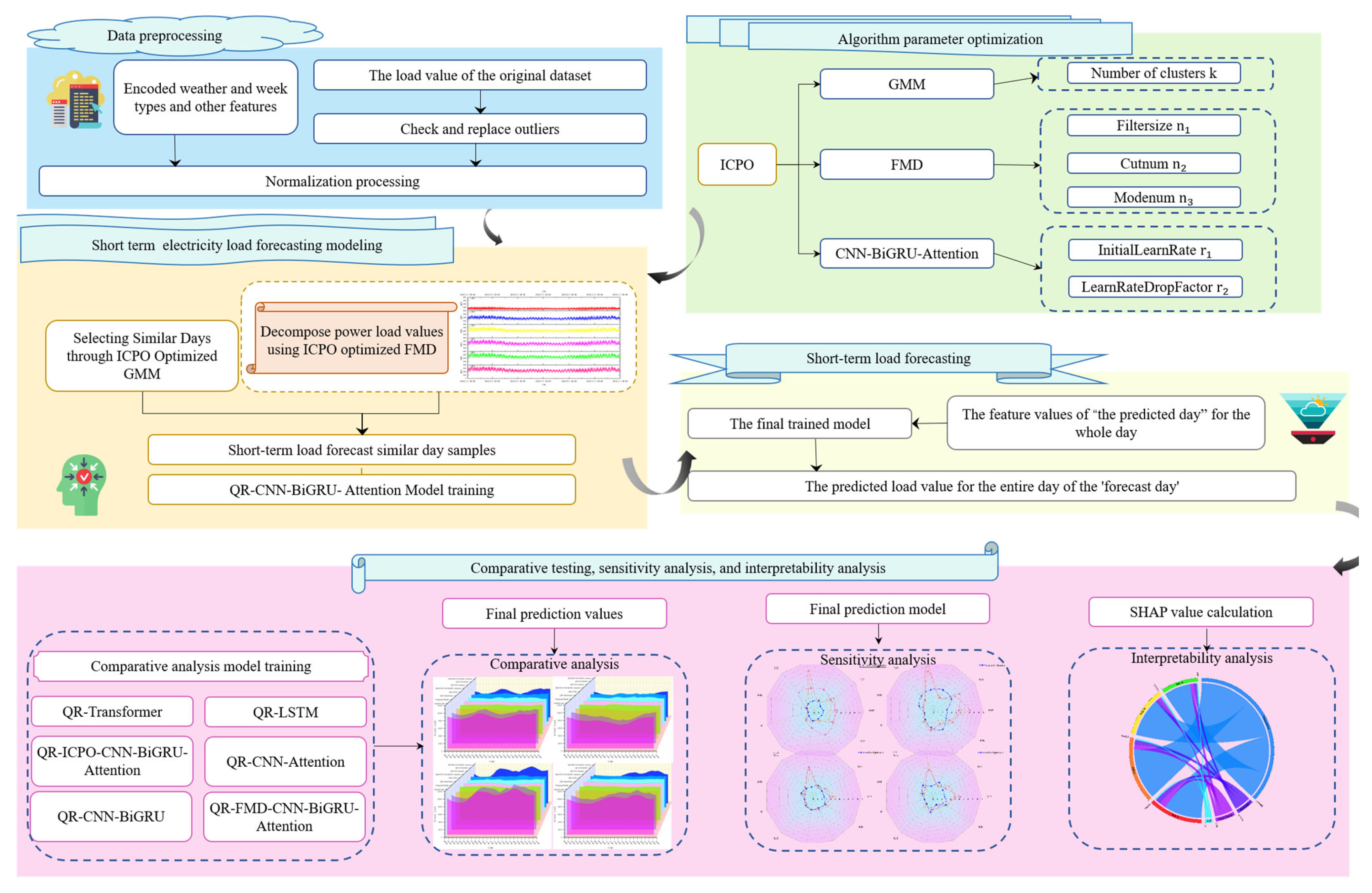
The strategic framework of the QR-CNN-BiGRU-Attention model is illustrated in Figure 1. By integrating CNN, BiGRU, and the Attention mechanism, the model extracts temporal features [30], captures bidirectional dependencies, and assigns weighted importance to key features, enhancing electricity load forecasting accuracy. Meanwhile, a 95% confidence interval-based quantile load forecasting approach is adopted, which characterizes the uncertainty of load forecasting by estimating upper and lower bound intervals. This mitigates the impact of outliers and noise on point forecasting, addressing the issue where point forecasts are susceptible to significant deviations due to anomalies and noise interference [31,32]. Consequently, this approach provides more comprehensive information for power system operation and scheduling.

Step 1: Data Preprocessing. This step involves encoding weather and weekday-type features, detecting and replacing outliers in load data, and performing normalization to generate a high-quality standardized dataset. These preprocessing procedures ensure consistency in the input data for subsequent modeling.

Step 2: Short-Term Electricity Load Forecasting Model Construction. First, the ICPO-optimized GMM is used to select historical dates with time point characteristics similar to the target forecasting day, forming a similar-day sample training set. Next, the ICPO-optimized FMD algorithm is applied to decompose the load values of similar-day samples, extracting Intrinsic Mode Functions (IMFs) and residual components as input features for the model. Finally, the similar-day features and decomposed load values are used to train the QR-CNN-BiGRU-Attention model.

Step 3: Short-Term Load Forecasting. The features of the target forecasting day are fed into the trained model to generate the predicted load components and their corresponding intervals for each time point throughout the day. The final daily load forecast is obtained by aggregating the component values and their intervals.

Step 4: Comparative Analysis and Validation. The proposed model’s forecasting performance is compared with other algorithms by computing evaluation metrics to assess its accuracy and effectiveness. Additionally, sensitivity and interpretability analyses are conducted to examine the impact of different features on the forecasting results, verifying the model’s reliability.

Figure 1. Strategic Framework of Short-Term Load Forecasting.

Figure 1. Strategic Framework of Short-Term Load Forecasting.

2.1. Data Preprocessing

The data preprocessing in this study includes outlier detection and normalization. Outliers, often caused by equipment failures or environmental changes, can significantly impact forecasting accuracy. Therefore, preprocessing these anomalies improves forecasting performance. To evaluate the effectiveness of interval forecasting in expressing the uncertainty associated with outliers, the forecasting results obtained from processed data are compared with those from unprocessed datasets [33]. Additionally, normalization ensures that all features are computed on the same scale, accelerating convergence and reducing the risk of overfitting.

2.1.1. Outlier Handling

Outlier detection is performed by examining the rate of change in load values between adjacent time points. If the rate exceeds a set threshold, the data point is labeled as an outlier, as shown in the following formula:

$$R_t={\displaystyle \frac{\left|x_t-x_{t-1}\right|}{x_{t-1}}}>\mathsf{\theta }$$

(1)

where $x_t$ is the load value at the current time step, $x_{t-1}$ is the load value at the previous time step, is the rate of change, and θ is set to 0.5.

If $x_t$ satisfies the above equation, it is considered an outlier. Once detected, the outlier is replaced using a moving average method.

2.1.2. Normalization

The mathematical expression for normalization is as follows:

$$x_i^{’}={\displaystyle \frac{x_i-\min \left(x\right)}{\max \left(x\right)-\min \left(x\right)}}$$

(2)

where $x_i$ is the i-th sample of the original data, $x_i^{’}$ is the normalized data, $\min \left(x\right)$ and $\max \left(x\right)$ are the minimum and maximum values of feature, respectively.

Normalization transforms the load values to the [0, 1] range, which helps accelerate convergence and reduce overfitting. The FMD algorithm effectively removes outliers and noise. Thus, no additional denoising is required.

2.2. Related Work

2.2.1. GMM

GMM is based on a probabilistic model that assumes the data comprises multiple Gaussian distributions. It models the data using mixing coefficients, mean values, and covariance parameters [34]. GMM employs the Expectation-Maximization algorithm for parameter estimation. In the Expectation step, the posterior probability of each data point belonging to each Gaussian component is calculated. Model parameters are updated based on the posterior probabilities in the Maximization step. This approach is highly effective for selecting similar days from the load dataset.

2.2.2. FMD

FMD is a novel signal decomposition method that utilizes an adaptive Finite Impulse Response filter to decompose the signal while combining kurtosis and impulsiveness for feature extraction. Compared to traditional methods such as Empirical Mode Decomposition and Variational Mode Decomposition, FMD performs better in handling non-stationary signals and removing mixed modes [35]. In electricity load forecasting, FMD decomposes the original time series into low-frequency trend components and high-frequency non-trend components, allowing deep learning models to process these components separately, thereby improving forecasting accuracy.

FMD iteratively updates the Finite Impulse Response filter coefficients to decompose the signal into multiple modes, capturing information at different time scales. This characteristic enables FMD to extract multi-level features from complex electricity load data, providing valuable support for subsequent forecasting. The following outlines the initialization steps and objective function of FMD:

(1)

Finite Impulse Response Filter Initialization

To decompose modes with specific frequencies and characteristics, FMD first initializes a set of Finite Impulse Response filters to decompose the different modes in the signal. The resulting mode components after decomposition can be represented by the convolution of the original signal with the filter coefficients, as shown in the following formula [35]:

$$m_k\left(t\right)={\displaystyle \sum }_{i=0}^{N-1}{h}_{i}x\left(t-i\right)$$

(3)

where $h_i$ is the filter’s coefficient, i.e., the weight of the FIR filter. These coefficients determine the filter’s frequency response, specifically which frequency components will be extracted from the signal. $x\left(t\right)$ is the original signal, representing the input signal to be decomposed.

(2)

Correlated Kurtosis(CK)

To ensure that the decomposed modes contain as much helpful information as possible, rather than noise or irrelevant modes, FMD introduces “Correlated Kurtosis” as the optimization objective for the decomposition [35]:

$${\mathrm{CK}}_k={\displaystyle \frac{E\left[{\left(m_k\left(t\right)-{\mu }_k\right)}^4\right]}{{\left(E\left[{\left(m_k\left(t\right)-{\mu }_k\right)}^2\right]\right)}^2}}$$

(4)

where $m_k\left(t\right)$ is the k-th mode, ${\mu }_k$ is the mean of the mode, and E represents the expectation operator.

This study uses FMD to decompose the original electricity load time series into multiple modes, which are inputs to the CNN-BiGRU-Attention model. By extracting feature patterns across multiple time scales, FMD helps the deep learning model more accurately capture the changing trends and detailed features within the electricity load data, thereby enhancing the accuracy of short-term load forecasting.

2.2.3. CNN

Numerous studies have proven that Convolutional Neural Networks (CNNs) effectively extract local patterns from time series data [36]. This study uses CNN to extract local temporal features from electricity load data. The model automatically learns local features through convolution operations, which help subsequent networks capture short-term fluctuations and local dependencies within the data. Its structure is illustrated in Figure 2.

The convolution operation in Figure 3 refers to applying filters (or convolution kernels) to local weight and summing the input features. The formula for this operation is [36]:

$${\mathrm{CK}}_k={\displaystyle \frac{E\left[{\left(m_k\left(t\right)-{\mu }_k\right)}^4\right]}{{\left(E\left[{\left(m_k\left(t\right)-{\mu }_k\right)}^2\right]\right)}^2}}$$

(5)

where $z_{ij}^{\left(k\right)}$ is the output value of the k-th convolutional kernel at position (i, j), $X$ is the input feature map, $w^{\left(k\right)}$ is the weight matrix of the k-th convolutional kernel, $b^{\left(k\right)}$ is the bias of the k-th convolutional kernel, and $M,N$ are the height and width of the k-th convolutional kernel.

The Pooling operation in Figure 3 refers to the pooling process used to reduce the dimensionality of the feature maps. The most commonly used methods are Max Pooling and Average Pooling. The formula for Average Pooling used in this study is as follows [36]:

$$p_{ij}={\displaystyle \frac{1}{M\cdot N}}{\displaystyle \sum }_{m=1}^M{\displaystyle \sum }_{n=1}^N{a}_{\left(i+m-1\right)\left(j+n-1\right)}$$

(6)

where $M$ and $N$ are the height and width of the pooling window.

Figure 3. BiGRU structure diagram.

Figure 3. BiGRU structure diagram.

2.2.4. BiGRU

Bidirectional Gated Recurrent Unit (BiGRU) is an improvement over the Gated Recurrent Unit (GRU), serving as a bidirectional variant of the GRU algorithm. BiGRU can simultaneously capture dependencies between past and future time steps. In contrast to the traditional unidirectional GRU, which can only learn from past information, BiGRU processes data bi-directionally, enabling it to capture better the bidirectional dependencies in electricity load data [37]. This characteristic is crucial in handling electricity load data with complex temporal dependencies. Its basic structure is illustrated in Figure 3.

Where $t$ represents the sequence length; $x_0$ to $x_t$ are the input sequence representing the time series data, with a feature vector input at each time step; $S_0$ to $S_t$ are the output sequence; $D_0$ to $D_t$ are the forward GRU module outputs; $U_0$ to $U_t$ are the backward GRU module outputs. The internal structure of the GRU module in Figure 3 is shown in the right-side block diagram, where the core components include the reset gate and the update gate:

(1)

Reset Gate

The reset gate controls how the new input is combined with the previous memory state [37]:

$$r_t=\sigma \left(W_r\cdot x_t+U_r\cdot h_{t-1}+b_r\right)r_t=\sigma \left(W_r\cdot x_t+U_r\cdot h_{t-1}+b_r\right)$$

(7)

where $x_t$ is the input at time step $t$, $h_{t-1}$ is the hidden state from the previous time step, $W_r,U_r$ is the weight matrix, $b_r$ is the bias term, and $\sigma$ is the sigmoid function.

(2)

Update Gate

The update gate determines to what extent the current hidden state should retain the previous hidden state [37]:

$$z_t=\sigma \left(W_z\cdot x_t+U_z\cdot h_{t-1}+b_z\right)$$

(8)

(3)

Candidate Hidden State

The candidate hidden state is a linear combination of the current input and the previous hidden state [37]:

$${\tilde{h}}_t=tanh\left(W_h\cdot x_t+U_h\cdot \left(r_t\otimes h_{t-1}\right)+b_h\right)$$

(9)

where $\otimes$ represents element-wise multiplication.

2.2.5. Attention Mechanism

To further improve the accuracy of the model’s electricity load forecasting, the Self-Attention (SE-Attention) mechanism is introduced [38]. The SE-Attention mechanism assigns different weights to the features at different time steps or time scales, allowing the model to focus on the most critical time steps and feature patterns for the current load forecasting task [38]. This mechanism effectively prevents the model from overfocusing on irrelevant or secondary information, thus enhancing the accuracy of the electricity load forecasting. Its basic structure is illustrated in Figure 4.

Where the input feature map is $X\in {ℝ}^{H\times W\times C}$, $H,W$ represent the height and width of the feature map, and $C$ is the number of channels; the output feature map of the SE-Attention is $Y\in {ℝ}^{H\times W\times C}$, having the same shape as the input. The input feature map first undergoes a convolution operation to extract features. A part of the output goes through the Squeeze and Excitation operations to obtain attention weights $s_c$, as shown in the upper branch of Figure 4. The other part is not processed and is multiplied element-wise with the attention weights $s_c$, resulting in the final output feature map.

2.2.6. Three-Strategy Improved CPO Algorithm and Its Optimization

The Crowned Crested Porcupine Optimization Algorithm (CPO) was innovatively proposed by Abdel-Basset et al. in 2024 [39]. The core of the CPO algorithm lies in its simulation of four defense strategies of the crowned Crested Porcupine (visual intimidation, auditory intimidation, olfactory attack, and physical attack), as shown in Figure 5. These strategies are applied progressively in the algorithm, corresponding to different stages of global exploration and local exploitation [39].

The mechanism of the CPO algorithm lies in its clever combination of global exploration and local exploitation search strategies. Simulating the defensive behaviors of the crowned Crested Porcupine achieves a balance between these two approaches, thus improving optimization efficiency. In this study, we improve upon the original CPO by incorporating chaos mapping, sine-cosine strategies, and cross-dimensional strategies, enriching the initial solutions and iteration process.

The chaos mapping strategy enhances the diversity of the initial population by generating complex search trajectories using chaotic mapping [40]. The sine-cosine strategy enables periodic oscillatory jumps, allowing individuals to explore the search space flexibly [41]. The crosswise strategy further improves solution diversity and global search efficiency through crossover operations between individuals [42]. The detailed explanations of these strategies are as follows.

Pseudocode for the Improved Crowned Crested Porcupine Optimization Algorithm 1 (ICPO):

Algorithm 1: CPO Optimization Algorithm for Three Strategy Optimization

Input: Initialize $N^{\prime },T_{max},\alpha ,T_f,T,N_{min};$ Use chaotic mapping to initialize the solutions’ positions, $X^i,i=1,2,\dots ,N$. Output: $\overrightarrow{x_i^{t+1}}$ $, \overrightarrow{x_{CP}^t}$.

1. While ($t<T_{max}$) do 2.   Evaluate fitness values for the candidate solutions; 3.   Determine the best ($\overrightarrow{x_{CP}^{\prime }}$) solution so far; 4.   Update ${\gamma }_t$ using ${\gamma }_t=2\times rand\times {\left(1-{\displaystyle \frac{t}{t_{max}}}\right)}^{{\displaystyle \frac{t}{t_{max}}}}$; 5.   Update the population size using $N=N_{min}+(N^{\prime }-N_{min})\times \left(1-\left({\displaystyle \frac{t\%\frac{T_{max}}{T}}{\frac{T_{max}}{T}}}\right)\right)$; 6.   For i = 1: N do 7.    Update the $m,S,F,\overrightarrow{\delta };$ 8.    Generate two random numbers, ${\tau }_8$ and ${\tau }_9$; 9.    If ${\tau }_8<{\tau }_9$ Then 10.     Generate two random numbers, ${\tau }_6$ and ${\tau }_7$; 11.    End If 12.    If ${\tau }_6<{\tau }_7$ Then 13.     Apply $\overrightarrow{x_i^{t+1}}=\overrightarrow{x_i^t}+{\tau }_1\times \left|2\times {\tau }_2\times \overrightarrow{x_{CP}^t}-\overrightarrow{y_i^t}\right|$; 14.     Else 15.     Apply $\overrightarrow{x_i^{t+1}}=\left(1-\overrightarrow{U_1}\right)\times \overrightarrow{x_i^t}+\overrightarrow{U_1}\times \left(\overrightarrow{y}+{\tau }_3\times \left(\overrightarrow{x_{r1}^t}-\overrightarrow{x_{r2}^t}\right)\right)$; 16.     Else 17.     Generate a random number, ${\tau }_{10}$; 18.    End If 19.    If ${\tau }_{10}<T_f$ Then 20.     Apply $\overrightarrow{x_i^{t+1}}=\left(1-\overrightarrow{U_1}\right)\times \overrightarrow{x_i^t}+\overrightarrow{U_1}\times \times \left(\overrightarrow{x_{r_1}^t}+S_i^t\times \left(\overrightarrow{x_{r_2}^t}-\overrightarrow{x_{r_3}^t}\right)-{\tau }_3\times \overrightarrow{\delta }\times {\gamma }_t\times S_i^t\right)$; 21.     Else 22.     Apply $\overrightarrow{x_i^{t+1}}=\overrightarrow{x_{CP}^t}+(\alpha (1-{\tau }_4)+{\tau }_4)\times \left(\delta \times \overrightarrow{x_{CP}^t}-\overrightarrow{x_i^t}\right)-{\tau }_5\times \delta \times {\gamma }_t\times \overrightarrow{F_i^t}$; 23.    End If 24.    If $f(\overrightarrow{x_i^{t+1}})>f(\overrightarrow{x_i^t})$ Then 25.     $\overrightarrow{x_i^{t+1}}=\overrightarrow{x_i^t}$; 26.    End If 27.    $t=t+1$; 28.   End for 29.  End while

Where $\overrightarrow{x_i^{t+1}}$ is the following solution in each iteration, $\overrightarrow{x_i^t}$ is the initial solution for each iteration; ${\tau }_1$, ${\tau }_2$, ${\tau }_3$, ${\tau }_4$, ${\tau }_5$, ${\tau }_6$ are random numbers between 0 and 1; $\overrightarrow{x_{CP}^t}$ is the fitness; $r$ is a random number between 1 and $N$; $N$ is the population size, which is set to 100 in this study; $\overrightarrow{\delta }$ controls the search direction; ${\gamma }_t$ is the defense factor; $S_t^i$ is the odor factor (simulating the crowned Crested Porcupine’s olfactory attack); $\alpha$ is the convergence speed factor.

This study employs ICPO to optimize the key hyperparameters of GMM, FMD, and the CNN-BiGRU-Attention model, as illustrated in Figure 6. The range of hyperparameters used in the experiments is determined based on multiple simulation trials and empirical selection, ensuring that the optimized decision variables do not fall on the boundary of the defined range. Further details can be found in Section 3.3.

2.3. Short-Term Load Interval Forecasting Model

2.3.1. Input Data Structure

This study utilizes the Belgium 2018 annual load dataset for interval-based time-series load forecasting (detailed data encoding in Section 3.1), with data sources from Elia Company (load and partial characteristics) [43] and “TimeAndDate” website (climate characteristics) [44]. The input sequence is constructed by combining the features and load values from the previous 24 h with the features of the current time step. The step size is set to 1 h, generating 24 forecasting results to obtain the load forecasting for the target day, as illustrated in Figure 7. In Figure 7, green and yellow dots represent the vectors and values of features and loads from time t-24 to time t+23, respectively.

2.3.2. Forecasting Model Framework

This study proposes a CNN-BiGRU-Attention quantile interval forecasting model to enhance the accuracy of short-term electricity load forecasting. The model optimizes performance by integrating CNN, BiGRU, and the Attention mechanism. CNN extracts local features and high-order patterns from time series data, BiGRU captures bidirectional dependencies, and the Attention mechanism dynamically focuses on key feature maps.

The proposed model employs quantile interval forecasting, providing both point and interval forecasting to quantify uncertainty, offering comprehensive support for power dispatching. As illustrated in Figure 8, the input data undergoes preprocessing before being fed into the model, which generates forecasting results. Finally, inverse normalization is applied to obtain the actual load values.

3. Simulation Analysis

3.1. Data Source

The dataset used in this experiment consists of the electricity load data for the entire year of 2018 in Belgium. The continuous characteristic trends of the yearly data are illustrated in Figure 9.

The dataset contains electricity load data for 24-time points per day throughout the year, covering seasonal variations and differences between weekdays and weekends in electricity demand. The forecasting target is electricity load, while the features include temperature, humidity, wind speed, and sea level pressure (raw data), along with weather categories, which are processed using One-Hot Encoding into a 30-dimensional representation. The features and load data are shown in Figure 9 and Figure 10, respectively.

This study selects samples with features similar to the target forecasting day as the training set, while the target forecasting day serves as the test set. To evaluate the model’s performance across different seasons and day types, we first extracted complete weeks (starting Monday, excluding cross-season weeks) from summer and winter, labeled these weeks, and randomly selected one week each from the two seasons—including a weekday and a weekend day from each season—then randomly picked a number from 1 to 5 (weekdays) and 6–7 (weekends), respectively, from the selected weeks, resulting in 4 days which are not included in the training set. The final four forecasting days chosen are July 12, July 14, December 11, and December 16.

3.2. Forecast Evaluation Metrics

To comprehensively assess the performance of the proposed model and compare it with recent algorithms, the following evaluation metrics are used in this experiment:

(1)

RMSE

RMSE measures the difference between the predicted and actual electricity load values. It is susceptible to more significant errors, making it a widely used metric in electricity load forecasting. The RMSE is defined as follows:

$$RMSE=\sqrt{{\displaystyle \frac{1}{n}}\sum _{i=1}^n{({\widehat{y}}_i-y_i)}^2}$$

(10)

where $y_i$ is the i-th actual value (observation), ${\widehat{y}}_i$ is the i-th predicted value, and $n$ is the total number of data points.

(2)

MAE

MAE measures the average magnitude of forecasting errors in electricity load forecasting, reflecting the model’s accuracy across different time points. It is defined as follows:

$$MAE={\displaystyle \frac{1}{n}}{\displaystyle \sum }_{i=1}^n\left|y_i-{\widehat{y}}_i\right|$$

(11)

where $y_i$ is the i-th actual value (observation), ${\widehat{y}}_i$ is the i-th predicted value, and $n$ is the total number of data points.

(3)

MAPE

MAPE represents the error as a percentage, measuring the model’s relative error in practical applications. It is defined as follows:

$$MAPE={\displaystyle \frac{1}{n}}\sum _{i=1}^n\left|{\displaystyle \frac{{\widehat{y}}_i-y_i}{y_i}}\right|\times 100\%$$

(12)

where $y_i$ is the i-th actual value (observation), ${\widehat{y}}_i$ is the i-th predicted value, and $n$ is the total number of data points.

(4)

PICP

This metric reflects the proportion of actual values that fall within the predicted interval, thereby assessing the reliability of the interval forecasting.

$$PICP={\displaystyle \frac{1}{n}}{\displaystyle \sum }_{i=1}^{n}I\left(y_i\in \left[{\widehat{y}}_i^{ \mathrm{lower}},{\widehat{y}}_i^{ \mathrm{upper}}\right]\right)$$

(13)

It represents the proportion of actual values that fall within the predicted interval and is used to measure the reliability of interval forecasting.

(5)

MPIW

$$MPIW={\displaystyle \frac{1}{n}}{\displaystyle \sum }_{i=1}^n{\displaystyle \frac{{\widehat{y}}_i^{ \mathrm{upper}}-{\widehat{y}}_i^{ \mathrm{lower}}}{{\widehat{y}}_i}}$$

(14)

It measures the width of the forecasting interval. A smaller relative width indicates that the model’s forecasting is more precise.

3.3. Model Selection and Hyperparameters

To validate the effectiveness of the improved algorithm model, this study compares the proposed algorithm with the following advanced forecasting models and a version of the proposed model with some components removed:

(1)

Transformer Quantile Regression Model

Utilizes the multi-head self-attention mechanism to capture long-term dependencies in time series and generate quantile intervals. Parameter settings refer to [45]: hidden neurons = 32, 3 hidden layers, batch size = 128, iterations = 1000, learning rate = 0.001.

(2)

LSTM Quantile Regression Model

It uses LSTM networks to capture long-term dependencies in time series, validating the improved model’s effect. The parameter settings refer to [46]: input length = 5, hidden layer nodes = 11, activation functions = Sigmoid and PURELIN, iterations = 200, and learning rate = 0.001.

(3)

ICPO-CNN-BiGRU-Attention

Based on the ICPO-optimized CNN-BiGRU-Attention model, it predicts load values by removing the FMD step. It combines CNN to extract local features, BiGRU to capture temporal dependencies, and the attention mechanism to focus on important information.

(4)

CNN-Attention Quantile Regression Model

A quantile regression model with only CNN and the Attention mechanism was used for ablation experiments. Parameter settings refer to [47]: number of convolutional filters = 64, kernel size = 3, max pooling window = 2, learning rate = 0.001, batch size = 128.

(5)

CNN-BiGRU Quantile Regression Model

A quantile regression model combining CNN and BiGRU without the Attention mechanism was used to assess the role of Attention. Parameter settings refer to [48]: dropout regularization = 0.5, optimizer = Adam, learning rate = 0.001, batch size = 128, iterations = 200.

(6)

FMD-CNN-BiGRU-Attention Quantile Regression Model

After decomposing load data, it is input into the CNN-BiGRU-Attention model, but without the ICPO algorithm, to analyze the impact of FMD. Parameter settings refer to [49]: number of convolutional filters = 4 and 8, BiGRU nodes = 10, Attention size = 64, learning rate = 0.001, batch size = 128, iterations = 100.

(7)

Proposed model

The hyperparameters of the proposed model are determined by ICPO, with the optimization strategy as shown in Figure 6 above.

①

ICPO Optimizing GMM Hyperparameters

The number of clusters k for GMM is optimized. The search range is limited to integer values between [3, 200], aiming to minimize the logarithmic error of the clustering, as described in Section 2.2.1. The final value of k is 19. The iterative process is illustrated in Figure 11. The core goal of this optimization is to minimize the logarithmic error of GMM clustering which serves as the dependent variable, quantifying the fitting degree between the GMM clustering result and the feature distribution of historical load data [34].

$$J_{\mathrm{GMM}}=-{\displaystyle \frac{1}{N}}{\displaystyle \sum }_{i=1}^N\ln \left({\displaystyle \sum }_{c=1}^k{\pi }_c\cdot \mathcal{N}\left(x_i;{\mu }_c;y_c\right)\right)$$

(15)

In the formula, N is the number of historical load samples; ${\pi }_c$ is the mixing coefficient of the c-th Gaussian component in GMM; $\mathcal{N}$ is the probability density function that the i-th sample belongs to the c-th Gaussian component; ${\mu }_c$ and $y_c$ are the mean and covariance matrix of the c-th Gaussian component, respectively.

Figure 11. Convergence Graph of ICPO Optimizing GMM.

Figure 11. Convergence Graph of ICPO Optimizing GMM.

②

ICPO Optimizing FMD Hyperparameters

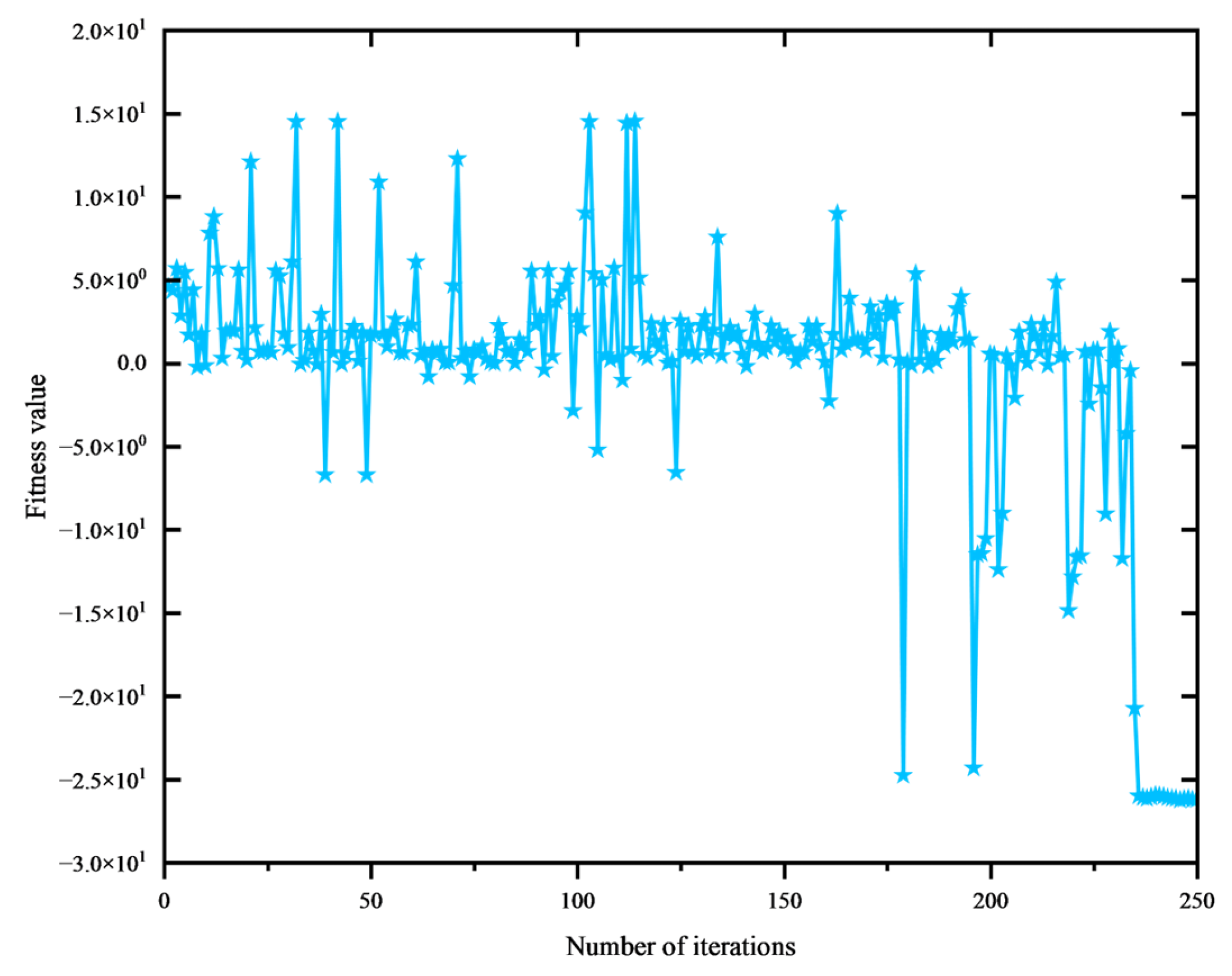
The optimization target is the inverse of the signal-to-noise ratio (SNR) of the FMD results. ICPO is used to optimize the hyperparameters of FMD, including the filter size $n_1$, the number of truncations $n_2$ and the number of modes $n_3$. The search ranges for these parameters are [1, 200], [1, 200], and [2, 200], respectively, with integer values. The final results are $n_1=3$, $n_2=6$, $n_3=10$, and an SNR of 26.0262 dB. The iterative process is illustrated in Figure 12. The objective function for this optimization is to maximize SNR [35], whose mathematical expression is:

$$J_{\mathrm{FMD}}=10\cdot {\log }_{10}\left({\displaystyle \frac{{{\displaystyle \sum }}_{t=1}^T{s}^2\left(t\right)}{{{\displaystyle \sum }}_{t=1}^T{n}^2\left(t\right)}}\right)$$

(16)

Here, $T$ is the length of the load time series; $s(t)$ represents the effective modal signal (IMF) after FMD; $n(t)$ represents the noise signal remaining after decomposition.

Figure 12. Convergence Graph of ICPO Optimizing FMD.

Figure 12. Convergence Graph of ICPO Optimizing FMD.

③

ICPO Optimizing CNN-BiGRU-Attention Hyperparameters

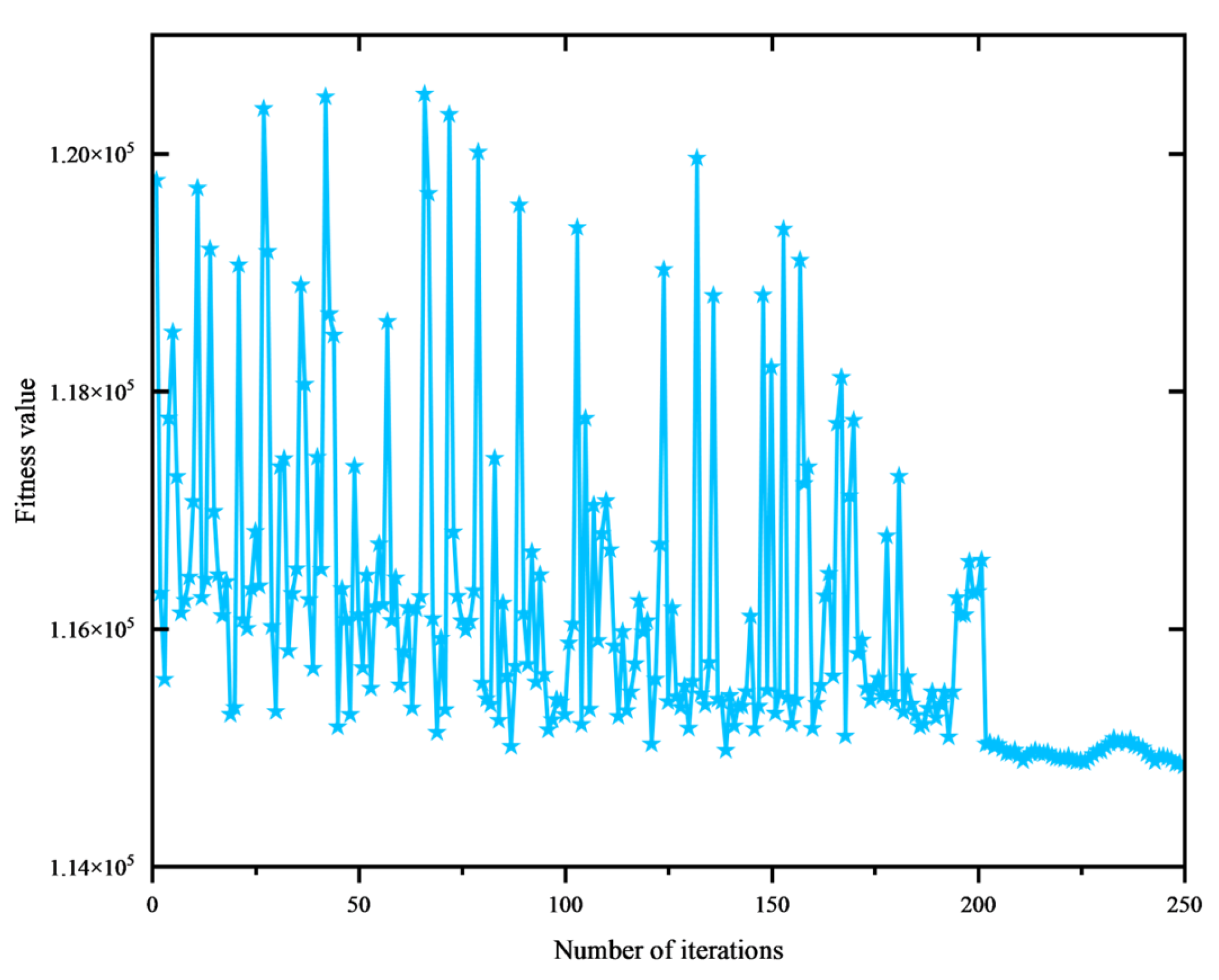
The optimization target is the RMSE between actual and predicted values. ICPO is used to optimize the key hyperparameters of the model, including the initial learning rate (${\mathrm{r}}_1$) and the learning rate drop factor (${\mathrm{r}}_2$). The search ranges for these parameters are [0.0001, 0.1] and [0.01, 0.5], respectively. The final results are ${\mathrm{r}}_1=0.01024$ and ${\mathrm{r}}_2=0.22$. The iterative process is illustrated in Figure 13. The objective function for this optimization is to minimize RMSE, calculated as:

Figure 13. Convergence Graph of ICPO Optimizing CNN-BiGRU-Attention.

Figure 13. Convergence Graph of ICPO Optimizing CNN-BiGRU-Attention.

$$J_{\mathrm{CNN}-\mathrm{BiGRU}}=\sqrt{{\displaystyle \frac{1}{N}}{\displaystyle \sum }_{i=1}^N{\left(y_i-{\widehat{y}}_i\right)}^2}$$

(17)

In the formula, N is the number of prediction samples; $y_i$ is the actual load value of the i-th sample; ${\widehat{y}}_i$ is the load value predicted by the CNN-BiGRU-Attention model for the i-th sample.

3.4. Forecasting Results Analysis

The simulation experiments in this study were conducted on the following equipment: Intel i7 13700KF CPU, NVIDIA TUF-RTX4070Ti-O16G GPU, 32 GB Kingston 3600 memory, 2 TB WD Sn770 storage, and Windows 11 Version 24H2 operating system. The simulation results are shown in Figure 14. The forecasting errors of various algorithms on different forecast days are shown in

Table 2. Forecasting errors of various algorithms on different forecast days.

Scene	Evaluation Index	Proposed Model	QR-LSTM	QR-ICPO-CNN-BiGRU-Attenion	QR-CNN-Attention	QR-CNN-BiGRU	QR-FMD-CNN-BiGRU-Attetnion	QR-Transformer
July 12th	RMSE	132.30	769.24	605.21	693.27	672.14	557.45	434.44
	MAE	120.53	655.12	505.01	577.06	549.01	477.80	421.25
	MAPE	1.40	7.44	5.74	6.52	6.20	5.48	4.94
	PICP	1.00	1.00	1.00	1.00	1.00	1.00	1.00
	MPIW	0.35	0.45	0.39	0.39	0.38	0.36	0.36
July 14th	RMSE	196.99	953.58	1072.33	1025.45	1119.60	1095.02	348.67
	MAE	157.61	837.21	887.43	868.58	935.38	913.25	337.86
	MAPE	2.18	11.96	12.89	12.55	13.56	13.23	4.57
	PICP	1.00	1.00	1.00	1.00	1.00	1.00	1.00
	MPIW	0.42	0.50	0.49	0.51	0.46	0.43	0.43
December 11th	RMSE	245.83	1680.13	1471.37	1615.36	1517.79	1494.24	548.29
	MAE	214.24	1500.60	290.00	158.68	140.25	141.68	1009.04
	MAPE	2.01	13.70	12.38	13.43	12.44	12.09	5.03
	PICP	0.89	0.83	0.88	0.82	0.83	0.79	0.82
	MPIW	0.36	0.41	0.42	0.44	0.40	0.43	0.43
December 16th	RMSE	220.99	791.43	799.62	864.16	774.04	778.22	367.34
	MAE	194.75	673.53	648.10	715.43	614.17	635.02	344.63
	MAPE	2.03	7.40	7.20	7.96	6.87	7.04	3.71
	PICP	1.00	1.00	1.00	1.00	1.00	1.00	1.00
	MPIW	0.43	0.45	0.45	0.48	0.45	0.43	0.43

.

Figure 14 and Figure 15 show that the proposed model demonstrates superior fitting performance compared to other models during different periods. Among them, the abscissa and ordinate of each point in Figure 15 correspond to the actual value and predicted value of the same time step. It effectively captures the actual load variation trends, and the point forecasting curve has a high degree of alignment with the actual load curve. According to the PICP in Table 2, the proposed interval forecasting algorithm provides higher reliability for each forecasting point than the comparison algorithms. The forecasting curves of the QR-Transformer and QR-LSTM models are relatively smoother, indicating that these models may not perform as well in handling high fluctuations in load compared to the model proposed in this paper. Models such as QR-CNN-BiGRU-Attention, QR-CNN-Attention, and QR-CNN-BiGRU also track the actual load variation trends to some extent but exhibit lower accuracy during critical load fluctuation periods.

(1)

Summer Weekdays and Weekends (Figure 14a,b)

On July 12 (weekday) and July 14 (weekend), the proposed model can predict the load peaks and valleys well and captures the periodic fluctuations of the load throughout the day. Other models show significant deviations in some key load peak or valley regions, especially during the morning and evening load peak periods. QR-Transformer and QR-LSTM models may have issues predicting load valleys, either overestimating or underestimating them, while QR-CNN-Attention and similar models display slightly delayed curves. The proposed model achieves a 100% PICP score and a minimal MPIW score, indicating accurate coverage while maintaining lower uncertainty.

(2)

Winter Weekdays and Weekends (Figure 14c,d)

On December 11 (weekday) and December 16 (weekend), the proposed model again demonstrated outstanding forecasting performance, particularly during peak periods and areas with significant fluctuations in the morning and evening. The forecasting curve of the proposed model closely aligns with the actual load curve. QR-LSTM and QR-Transformer models showed relatively poor forecasting accuracy during load valleys, failing to fully follow the actual load valley trend and exhibiting some delay or over-smoothing. QR-FMD-CNN-BiGRU-Attention performed similarly to the proposed model, indicating that FMD and the Attention mechanism help improve forecasting accuracy. The proposed model achieved the highest PICP score on both days and the lowest MPIW score on December 16, indicating accurate coverage and relatively low uncertainty. Although the proposed model’s MPIW score on December 11 was not the lowest among all, the highest PICP score shows that the model improved coverage by appropriately expanding the interval width. This trade-off could be due to higher load fluctuations and inherent uncertainty on that day.

Figure 15. The Actual and Predicted Values of the Proposed Algorithm.

Figure 15. The Actual and Predicted Values of the Proposed Algorithm.

The proposed model showed strong forecasting ability across all periods, particularly in capturing load peaks, valleys, and other high-volatility periods. By incorporating FMD, Attention mechanisms, BiGRU, and ICPO-optimized models (i.e., the Proposed Model), the model effectively handles the non-linearity and volatility in load data. While capable of forecasting, traditional QR-LSTM and QR-Transformer models performed worse than the proposed model during high-volatility periods, mainly exhibiting over-smoothing or delay. QR-CNN-Attention and QR-CNN-BiGRU models showed improved accuracy but faced limitations in handling complex load fluctuations.

The proposed improved model performed best in forecasting accuracy, volatility tracking, and capturing high and low load periods, demonstrating that incorporating FMD, BiGRU, Attention mechanisms, and the ICPO algorithm’s integrated strategy significantly enhances forecasting performance in short-term load forecasting.

3.5. Sensitivity Analysis

Sensitivity analysis assesses the impact of small changes in input variables on the model’s output. In this study, other features were kept constant while a designated percentage adjusted a specific feature. MAPE was calculated to identify the features most sensitive to electricity load forecasting results. The analysis was performed for four features on the four forecasting days, with the results shown in Figure 16. It can be seen that when the adjustment magnitude is 0%, MAPE is minimized, but the error does not always increase with the adjustment magnitude. Overall, the forecasting results are most sensitive to temperature and humidity.

3.6. Interpretability Analysis

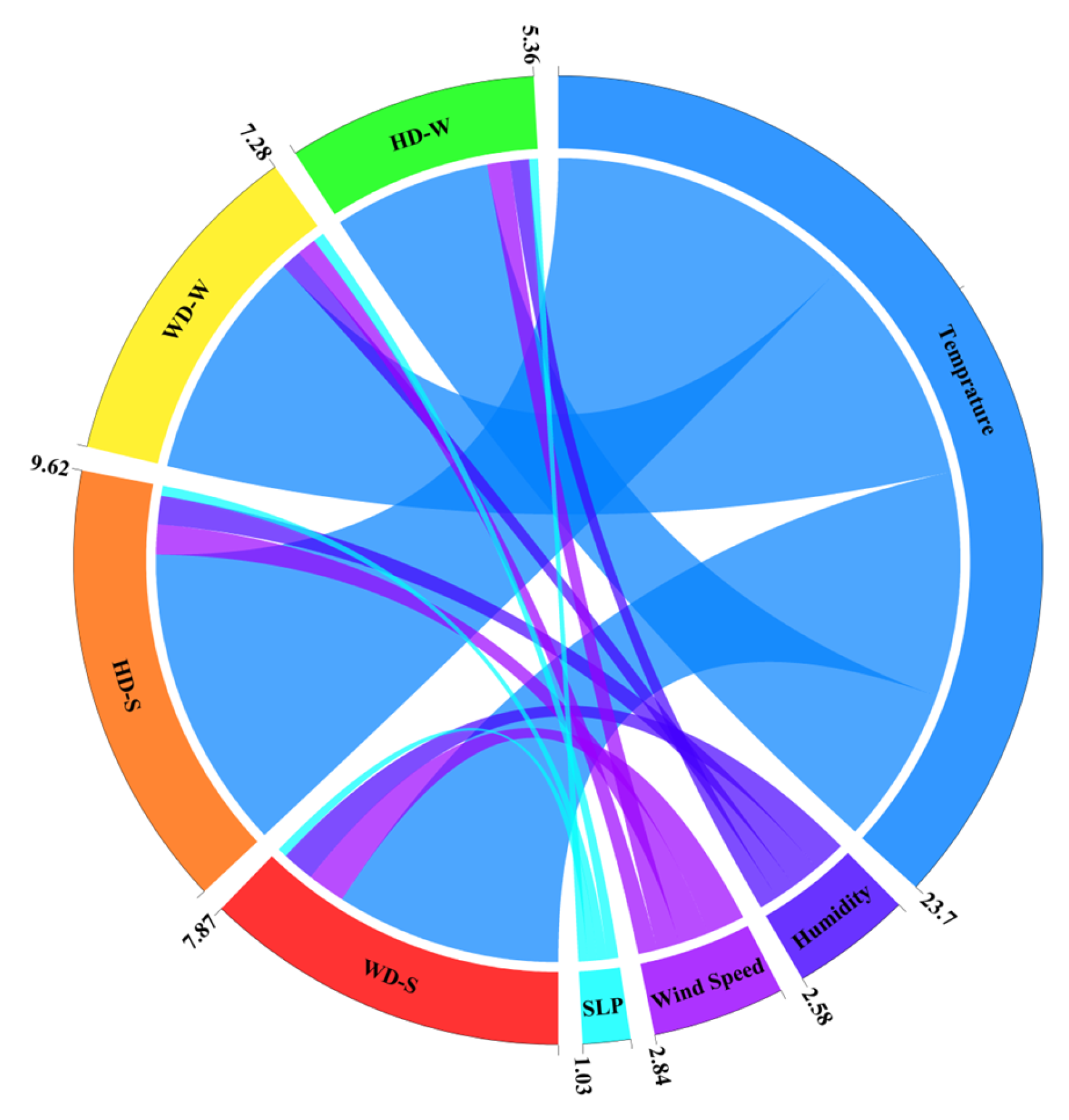
To improve the interpretability of the model, this study uses a chord diagram for analysis, as shown in Figure 17. The diagram contains eight rings, with four feature rings, including Temperature, Humidity, Wind Speed, and Sea Level Pressure (SLP). The other four rings represent forecasting days: Winter Working Days (WD-W), Summer Working Days (WD-S), Winter Holidays (HD-W), and Summer Holidays (HD-S). The chords between the feature rings and the forecasting day rings represent the extent to which each feature influences the forecasting day, with the thickness of the chord reflecting the strength of the influence. The values on the outer side of the rings are SHAP values.

To calculate the impact of each feature on different forecasting days, this study uses Shapley (SHAP) values to analyze the influence of each feature quantitatively. For the i-th feature vector, its SHAP value ${\varphi }_i\left(x\right)$ can be computed using the following formula:

$${\varphi }_i\left(x\right)={\displaystyle \sum _{S\subseteq N\backslash \left\{i\right\}}\frac{\left|S\right|!\left(m-\left|S\right|-1\right)!}{m!}}\left[f\left(S\cup \left\{i\right\}\right)-f\left(S\right)\right]$$

(18)

where $N=\left\{1,2,\dots ,m\right\}$ is the set of all features. S is an arbitrary subset of the feature set N, and $i\notin S$. f(S) is the model’s forecasting on the subset S (i.e., forecasting is made using only the features in subset S); $f\left(S\cup \left\{i\right\}\right)$ is the model’s forecasting on the subset S and feature i. $\left|S\right|$ is the size of subset S. The weight ${\displaystyle \frac{\left|S\right|!\left(m-\left|S\right|-1\right)!}{m!}}$ is the combination weight, representing the probability of the subset S appearing.

Based on Figure 17, temperature has the most significant impact on the four forecasting days, with its influence being slightly higher in summer than in winter. The effects of wind speed and humidity are pretty consistent, with wind speed having a slightly more significant effect than humidity, and again, the impact is more substantial in summer than in winter. Sea level pressure has the least impact, showing almost no difference across the four forecasting days, and can be considered negligible.

4. Conclusions

Improved Crowned Crested Porcupine Optimization Algorithm (ICPO) integrated with Feature Mode Decomposition (FMD) and deep learning (QR-ICPO-FMD-CNN-BiGRU-Attention) for short-term electricity load forecasting was studied in this research paper. The original CPO algorithm was improved by introducing chaos strategies, chaos sine-cosine cross strategies, and golden sine strategies, significantly enhancing its global search capability and optimization efficiency. The research results indicate that this model outperforms the comparison models in several metrics (RMSE, MAE, MAPE, PICP and MPIW), demonstrating strong generalization and adaptability and providing higher accuracy and stability for short-term load forecasting. The specific findings include:

(1)

Effectiveness of the Improved Optimization Algorithm

The load forecasting results show that the improved ICPO algorithm exhibits excellent optimization capabilities, and the performance of the model is significantly enhanced. Better forecasting results are delivered by the model across various complex load scenarios.

(2)

Model Integration and Performance Improvement

By integrating FMD with deep learning models, the decomposition, clustering, optimization, and forecasting modules work efficiently together. For the improved ICPO-FMD-CNN-BiGRU-Attention model, at least a 39.84% improvement in RMSE, 26.12% in MAE, and 45.28% in MAPE is achieved.

(3)

Model Adaptability and Robustness

The PICP and MPIW metrics of the proposed model are improved by at least 3.80% and 2.27%, respectively. This indicates that the information density and practical value of the forecasting intervals are significantly enhanced by the model while a 95% confidence level is ensured. Furthermore, the reliability and uncertainty analysis of the forecasting results shows that the model not only outperforms comparison models in terms of accuracy but also demonstrates stronger adaptability and robustness in complex load fluctuation scenarios, and reliable support is provided for short-term electricity load forecasting.

Although strong performance is shown by the proposed model, limitations in computational complexity, data dependency, and scenario generalization still exist. Future work may involve the simplification of the model, efficient data processing, and broader scenario validation, so as to enhance its practicality and adaptability.

References

1. Tang, J.; Saga, R.; Cai, H.; Ma, Z.; Yu, S. Advanced integration of forecasting models for sustainable load forecasting in large-scale power systems. Sustainability 2024, 16, 1710. [Google Scholar] [CrossRef]
2. Mordjaoui, M.; Haddad, S.; Medoued, A.; Laouafi, A. Electric load forecasting by using dynamic neural network. Int. J. Hydrogen Energy 2017, 42, 17655–17663. [Google Scholar] [CrossRef]
3. Han, L.; Peng, Y.; Li, Y.; Yong, B.; Zhou, Q.; Shu, L. Enhanced deep networks for short-term and medium-term load forecasting. IEEE Access 2019, 7, 4045–4055. [Google Scholar] [CrossRef]
4. Wang, C.; Zhao, H.; Liu, Y.; Fan, G. Minute-level ultra-short-term power load forecasting based on time series data features. Appl. Energy 2024, 372, 123801. [Google Scholar] [CrossRef]
5. Rafi, S.H.; Masood, N.A.; Deeba, S.R.; Hossain, E. A Short-Term load forecasting method using integrated CNN and LSTM network. IEEE Access 2021, 9, 32436–32448. [Google Scholar] [CrossRef]
6. Saxena, A.; Shankar, R.; El-Saadany, E.F.; Kumar, M.; Al Zaabi, O.; Al Hosani, K.; Muduli, U.R. Intelligent load forecasting and renewable energy integration for enhanced grid reliability. IEEE Trans. Ind. Appl. 2024, 60, 8403–8417. [Google Scholar] [CrossRef]
7. Yin, L.; Xie, J. Multi-temporal-spatial-scale temporal convolution network for short-term load forecasting of power systems. Appl. Energy 2021, 283, 116328. [Google Scholar] [CrossRef]
8. Eren, Y.; Küçükdemiral, İ. A comprehensive review on deep learning approaches for short-term load forecasting. Renew. Sustain. Energy Rev. 2024, 189 Pt B, 114031. [Google Scholar] [CrossRef]
9. Parmezan, A.R.S.; Souza, V.M.A.; Batista, G.E.A.P.A. Evaluation of statistical and machine learning models for time series forecasting: Identifying the state-of-the-art and the best conditions for using each model. Inf. Sci. 2019, 484, 302–337. [Google Scholar] [CrossRef]
10. Memarzadeh, G.; Keynia, F. Short-term electricity load and price forecasting by a new optimal LSTM-NN based forecasting algorithm. Electr. Power Syst. Research 2021, 192, 106995. [Google Scholar] [CrossRef]
11. Dhaval, B.; Deshpande, A. Short-term load forecasting using multiple linear regression. Int. J. Electr. Comput. Eng. 2020, 10, 3911. [Google Scholar] [CrossRef]
12. Xie, Z.; Wang, R.; Wu, Z.; Liu, T. Short-Term power load forecasting model based on fuzzy neural network using improved decision tree. In Proceedings of the 2019 IEEE Sustainable Power and Energy Conference (iSPEC), Beijing, China, 21–23 November 2019; pp. 482–486. [Google Scholar]
13. Samantaray, S.; Sahoo, A.; Satapathy, D.P.; Oudah, A.Y.; Yaseen, Z.M. Suspended sediment load forecasting using sparrow search algorithm-based support vector machine model. Sci. Rep. 2024, 14, 12889. [Google Scholar] [CrossRef] [PubMed]
14. Si, C.; Wang, H.; Chen, L.; Zhao, J.; Min, Y.; Xu, F. Robust co-modeling for privacy-preserving short-term load forecasting with incongruent load data distributions. IEEE Trans. Smart Grid 2024, 15, 2985–2999. [Google Scholar] [CrossRef]
15. Chen, Z.; Chen, Y.; Xiao, T.; Wang, H.; Hou, P. A novel short-term load forecasting framework based on time-series clustering and early classification algorithm. Energy Build. 2021, 251, 111375. [Google Scholar] [CrossRef]
16. Yang, Y.; Wang, Z.; Gao, Y.; Wu, J.; Zhao, S.; Ding, Z. An effective dimensionality reduction approach for short-term load forecasting. Electr. Power Syst. Res. 2022, 210, 108150. [Google Scholar] [CrossRef]
17. Li, W.; Zuo, Y.; Su, T.; Zhao, W.; Ma, X.; Cui, G.; Wu, J.; Song, Y. Firefly Algorithm-based semi-supervised learning with transformer method for shore power load forecasting. IEEE Access 2023, 11, 77359–77370. [Google Scholar] [CrossRef]
18. Pang, X.; Sun, W.; Li, H.; Liu, W.; Luan, C. Short-term power load forecasting method based on Bagging-stochastic configuration networks. PLoS ONE 2024, 19, e0300229. [Google Scholar] [CrossRef]
19. Luo, S.; Wang, B.; Gao, Q.; Wang, Y.; Pang, X. Stacking integration algorithm based on CNN-BiLSTM-Attention with XGBoost for short-term electricity load forecasting. Energy Rep. 2024, 12, 2676–2689. [Google Scholar] [CrossRef]
20. Mamun, A.A.; Sohel, M.; Mohammad, N.; Sunny, S.H.; Dipta, D.R.; Hossain, E. A comprehensive review of the load forecasting techniques using single and hybrid predictive models. IEEE Access 2020, 8, 134911–134939. [Google Scholar] [CrossRef]
21. Bu, X.; Wu, Q.; Zhou, B.; Li, C. Hybrid short-term load forecasting using CGAN with CNN and semi-supervised regression. Appl. Energy 2023, 338, 120920. [Google Scholar] [CrossRef]
22. Sekhar, C.; Dahiya, R. Robust framework based on hybrid deep learning approach for short term load forecasting of building electricity demand. Energy 2023, 268, 126660. [Google Scholar] [CrossRef]
23. Shakeel, A.; Chong, D.; Wang, J. District heating load forecasting with a hybrid model based on LightGBM and FB-prophet. J. Clean. Prod. 2023, 409, 137130. [Google Scholar] [CrossRef]
24. Han, F.; Pu, T.; Li, M.; Taylor, G. Short-term forecasting of individual residential load based on deep learning and K-means clustering. CSEE J. Power Energy Syst. 2020, 7, 261–269. [Google Scholar]
25. Hu, L.; Wang, J.; Guo, Z.; Zheng, T. Load forecasting based on LVMD-DBFCM load curve clustering and the CNN-IVIA-BLSTM Model. Appl. Sci. 2023, 13, 7332. [Google Scholar] [CrossRef]
26. Han, Z.; Cheng, M.; Chen, F.; Wang, Y.; Deng, Z. A spatial load forecasting method based on DBSCAN clustering and NAR neural network. J. Phys. Conf. Ser. 2020, 1449, 012032. [Google Scholar] [CrossRef]
27. Bedi, J.; Toshniwal, D. Energy load time-series forecast using decomposition and autoencoder integrated memory network. Appl. Soft Comput. 2020, 93, 106390. [Google Scholar] [CrossRef]
28. Chen, H.; Huang, H.; Zheng, Y.; Yang, B. A load forecasting approach for integrated energy systems based on aggregation hybrid modal decomposition and combined model. Appl. Energy 2024, 375, 124166. [Google Scholar] [CrossRef]
29. Yang, D.; Guo, J.; Li, Y.; Sun, S.; Wang, S. Short-term load forecasting with an improved dynamic decomposition-reconstruction-ensemble approach. Energy 2023, 263, 125609. [Google Scholar] [CrossRef]
30. Liu, Y.; Pu, H.; Sun, D.W. Efficient extraction of deep image features using convolutional neural network (CNN) for applications in detecting and analysing complex food matrices. Trends Food Sci. Technol. 2021, 113, 193–204. [Google Scholar] [CrossRef]
31. Lin, J.; Ma, J.; Zhu, J.; Cui, Y. Short-term load forecasting based on LSTM networks considering attention mechanism. Int. J. Electr. Power Energy Syst. 2022, 137, 107818. [Google Scholar] [CrossRef]
32. Ma, X.; Dong, Y. An estimating combination method for interval forecasting of electrical load time series. Expert Syst. Appl. 2020, 158, 113498. [Google Scholar] [CrossRef]
33. Dong, F.; Wang, J.; Xie, K.; Tian, L.; Ma, Z. An interval forecasting method for quantifying the uncertainties of cooling load based on time classification. J. Build. Eng. 2022, 56, 104739. [Google Scholar] [CrossRef]
34. Zhang, Y.; Li, M.; Wang, S.; Dai, S.; Luo, L.; Zhu, E.; Xu, H.; Zhu, X.; Yao, C.; Zhou, H. Gaussian mixture model clustering with incomplete data. ACM Trans. Multimed. Comput. Commun. Appl. 2021, 17, 6. [Google Scholar] [CrossRef]
35. Miao, Y.; Zhang, B.; Li, C.; Lin, J.; Zhang, D. Feature mode decomposition: New decomposition theory for rotating machinery fault diagnosis. IEEE Trans. Ind. Electron. 2023, 70, 1949–1960. [Google Scholar] [CrossRef]
36. Kattenborn, T.; Leitloff, J.; Schiefer, F.; Hinz, S. Review on Convolutional Neural Networks (CNN) in vegetation remote sensing. ISPRS J. Photogramm. Remote Sens. 2021, 173, 24–49. [Google Scholar] [CrossRef]
37. Zou, Z.; Wang, J.; Ning, E.; Zhang, C.; Wang, Z.; Jiang, E. Short-Term power load forecasting: An integrated approach utilizing variational mode eecomposition and TCN–BiGRU. Energies 2023, 16, 6625. [Google Scholar] [CrossRef]
38. Niu, Z.; Zhong, G.; Yu, H. A review on the attention mechanism of deep learning. Neurocomputing 2021, 452, 48–62. [Google Scholar] [CrossRef]
39. Abdel-Basset, M.; Mohamed, R.; Abouhawwash, M. Crested Porcupine Optimizer: A new nature-inspired metaheuristic. Knowl. Based Syst. 2024, 284, 111257. [Google Scholar] [CrossRef]
40. Li, C.; Feng, B.; Li, S.; Kurths, J.; Chen, G. Dynamic Analysis of Digital Chaotic Maps via State-Mapping Networks. IEEE Trans. Circuits Syst. I Regul. Pap. 2019, 66, 2322–2335. [Google Scholar] [CrossRef]
41. Singh, N.; Kaur, J. Hybridizing sine-cosine algorithm with harmony search strategy for optimization design problems. Soft Comput. 2021, 25, 11053–11075. [Google Scholar] [CrossRef]
42. Zhou, Z.; Jia, Y.; Lu, W.; Lei, J.; Liu, Z. Enhancing the crack initiation resistance of hydrogels through crosswise cutting. J. Mech. Phys. Solids 2024, 183, 105516. [Google Scholar] [CrossRef]
43. ELIA. Measured and Forecasted Total Load on the Belgian Grid (Historical Data). Available online: https://opendata.elia.be/explore/dataset/ods001/analyze/?dataChart=eyJxdWVyaWVzIjpbeyJjaGFydHMiOlt7InR5cGUiOiJsaW5lIiwiZnVuYyI6IkFWRyIsInlBeGlzIjoidG90YWxsb2FkIiwic2NpZW50aWZpY0Rpc3BsYXkiOnRydWUsImNvbG9yIjoiI2U3NTQyMCJ9XSwieEF4aXMiOiJkYXRldGltZSIsIm1heHBvaW50cyI6bnVsbCwidGltZXNjYWxlIjoibW9udGgiLCJzb3J0IjoiIiwiY29uZmlnIjp7ImRhdGFzZXQiOiJvZHMwMDEiLCJvcHRpb25zIjp7fX19XSwiZGlzcGxheUxlZ2VuZCI6dHJ1ZSwiYWxpZ25Nb250aCI6dHJ1ZX0%3D (accessed on 15 March 2024).
44. Timeanddate. Weather in Belgium. Available online: https://www.timeanddate.com/weather/belgium (accessed on 15 March 2024).
45. Ran, P.; Dong, K.; Liu, X.; Wang, J. Short-term load forecasting based on CEEMDAN and Transformer. Electr. Power Syst. Res. 2023, 214, 108885. [Google Scholar] [CrossRef]
46. Jin, Y.; Guo, H.; Wang, J.; Song, A. A Hybrid System Based on LSTM for Short-Term power load forecasting. Energies 2020, 13, 6241. [Google Scholar] [CrossRef]
47. Lin, Z. A hybrid CNN-LSTM-Attention model for electric energy consumption forecasting. In Proceedings of the 2023 5th Asia Pacific Information Technology Conference, Ho Chi Minh, Vietnam, 9–11 February 2023; pp. 167–173. [Google Scholar]
48. Li, C.; Li, G.; Wang, K.; Han, B. A multi-energy load forecasting method based on parallel architecture CNN-GRU and transfer learning for data deficient integrated energy systems. Energy 2022, 259, 124967. [Google Scholar] [CrossRef]
49. Niu, D.; Yu, M.; Sun, L.; Gao, T.; Wang, K. Short-term multi-energy load forecasting for integrated energy systems based on CNN-BiGRU optimized by attention mechanism. Appl. Energy 2022, 313, 118801. [Google Scholar] [CrossRef]
Figure 2. CNN architecture diagram.
Algorithms 18 00659 g002
Figure 4. Self-attention mechanism architecture diagram.
Algorithms 18 00659 g004
Figure 5. Strategy diagram of the three-strategy optimized CPO algorithm.
Algorithms 18 00659 g005
Figure 6. ICPO Optimization Strategy Diagram for Various Algorithms.
Algorithms 18 00659 g006
Figure 7. Input Structure of the Load Forecasting Model.
Algorithms 18 00659 g007
Figure 8. CNN-BiGRU-Attention Architecture.
Algorithms 18 00659 g008
Figure 9. The Average Feature Data Over Time.
Algorithms 18 00659 g009aAlgorithms 18 00659 g009b
Figure 10. The Average Load Over Time.
Algorithms 18 00659 g010
Figure 14. Comparison of actual and predicted values of various algorithms.
Algorithms 18 00659 g014
Figure 16. Sensitivity Analysis of Each Feature.
Algorithms 18 00659 g016
Figure 17. SHAP Interpretability Analysis.
Algorithms 18 00659 g017