Artificial Intelligence-Driven Diagnostics in Eye Care: A Random Forest Approach for Data Classification and Predictive Modeling

Abstract

Artificial intelligence and machine learning have increasingly transformed optometry, enabling automated classification and predictive modeling of eye conditions. In this study, we introduce Optometry Random Forest, an artificial intelligence-based system for automated classification and forecasting of optometric data. The proposed methodology leverages Random Forest models, trained on academic optometric datasets, to classify key diagnostic categories, including Contactology, Dry Eye, Low Vision, Myopia, Pediatrics, and Refractive Surgery. Additionally, an autoRegressive integrated moving average based forecasting model is incorporated to predict future research trends in optometry until 2030. Comparing the one-shot and epoch-trained Optometry Random Forest, the findings indicate that the epoch-trained model consistently outperforms the one-shot model, achieving superior classification accuracy (97.17%), precision (97.28%), and specificity (100%). Moreover, the comparative analysis with Optometry Bidirectional Encoder Representations from Transformers demonstrates that the Optometry Random Forest excels in classification reliability and predictive analytics, positioning it as a robust artificial intelligence tool for clinical decision-making and resource allocation. This research highlights the potential of Random Forest models in medical artificial intelligence, offering a scalable and interpretable solution for automated diagnosis, predictive analytics, and artificial intelligence-enhanced decision support in optometry. Future work should focus on integrating real-world clinical datasets to further refine classification performance and enhance the potential for artificial intelligence-driven patient care.

1. Introduction

In recent years, artificial intelligence (AI) and machine learning (ML) have significantly transformed various fields of medicine, including ophthalmology and optometry [1]. Among these technologies, the Random Forest (RF) algorithm has emerged as a powerful tool for classification and prediction in the diagnosis and management of ocular diseases such as glaucoma and myopia [2,3]. The integration of ML techniques into optometry has led to substantial improvements in diagnostic accuracy, risk assessment, and personalized treatment strategies. ML has revolutionized various medical fields, including optometry and ophthalmology, by enhancing diagnostic accuracy and patient care [4]. Among ML algorithms, RF has emerged as a powerful tool due to its robustness and ability to handle complex datasets. Originally introduced by Breiman [5], RF operates by constructing multiple decision trees and aggregating their outputs to achieve high classification accuracy. Unlike traditional regression models, which assume linearity and independence among predictor variables, RF is well suited for analyzing highly interdependent medical data, making it particularly effective in ophthalmic imaging, raw data analysis, and disease classification [6].

Glaucoma is one of the leading causes of blindness worldwide, characterized by progressive loss of retinal ganglion cells (RGCs) and thinning of the circumpapillary retinal nerve fiber layer (cpRNFL) before detectable visual field (VF) defects occur [7]. Early detection is crucial in preventing irreversible vision loss. Optical coherence tomography (OCT) has become a key imaging modality in diagnosing glaucoma by measuring structural changes in the optic nerve head and retinal layers. Traditional statistical models such as logistic regression and Support Vector Machines (SVM) have been used to identify glaucomatous changes. However, RF has demonstrated superior performance in handling correlated data and improving diagnostic accuracy [8,9]. Dry eye syndrome is another condition where RF has been utilized to improve diagnostic accuracy. Traditional dry eye assessments often involve invasive and subjective tests, but RF-based models have been developed to analyze non-invasive imaging data. A recent study demonstrated that ultrasound imaging combined with RF segmentation algorithms significantly improved dry eye syndrome detection [10]. These models provide an automated, objective method for diagnosing dry eye, reducing reliance on subjective patient-reported symptoms.

RF is an ensemble learning method that constructs multiple decision trees using randomly selected subsets of training data. This approach mitigates the issue of overfitting, which is a common limitation of single decision tree models, leading to enhanced classification performance in complex clinical datasets [8]. Recent studies have shown the effectiveness of RF in diagnosing glaucoma using OCT-derived structural measurements, with high sensitivity and specificity in distinguishing early-stage glaucomatous eyes from healthy controls [3,9]. A major challenge in glaucoma detection is the significant overlap between OCT parameters in normal and glaucomatous eyes, making simple threshold-based classification unreliable. RF models, which integrate multiple predictive variables, have proven effective in capturing complex patterns within these datasets. Furthermore, deep learning-based models incorporating fundus photography and OCT imaging have been developed, complementing RF classifiers to enhance early detection rates [9]. The implementation of RF in glaucoma diagnostics has not only improved early detection but also optimized disease progression monitoring and treatment planning [11].

Myopia has become a global public health issue, particularly in East Asia, where its prevalence has reached alarming levels [12]. Large-scale epidemiological studies have leveraged RF to predict myopia onset and progression by analyzing ocular biometric parameters such as axial length, corneal curvature, and exposure to natural light [13]. By integrating data from multiple sources, RF models provide more accurate predictions compared to traditional regression models, making them valuable tools in preventive optometry. In clinical practice, subjective refraction remains the gold standard for prescribing corrective lenses, but its accuracy heavily depends on the initial objective refraction measurements. In many regions, retinoscopy is not widely practiced, and autorefractors are commonly used as an alternative. However, autorefractors often introduce measurement errors, particularly in pediatric populations with high accommodative responses. To address this issue, RF regression models have been developed to refine autorefractor measurements, improving the precision of subjective refraction [11].

Additionally, RF has been used in public health research to evaluate environmental and genetic risk factors contributing to myopia development. Longitudinal studies employing RF have analyzed how urbanization, near-work activities, and outdoor exposure influence myopia progression [14] By leveraging machine learning, these studies provide valuable insights into potential intervention strategies, such as school-based outdoor activity programs aimed at reducing myopia incidence.

The use of RF in optometry offers several advantages. First, its ability to handle large datasets with highly correlated variables makes it particularly suited for medical applications where multiple factors influence disease outcomes. Second, RF’s ensemble approach reduces the risk of overfitting, leading to improved generalization when applied to independent datasets. Additionally, RF provides interpretability by ranking the importance of individual predictors, facilitating the identification of key diagnostic features in clinical assessments [2].

In [15] authors proposed a methodology for classifying optometry-related data and leveraging this structured information to develop an AI-driven diagnostic system. Their approach demonstrated the potential of AI in automated diagnostic decision-making by extracting meaningful patterns from optometric datasets, which provides a proposal for the foundation for integrating machine learning models into clinical workflows. Building upon this framework, refs. [15,16] employs a deep learning-based approach, similar to authors in [17], utilizing Bidirectional Encoder Representations from Transformers (BERT) to enhance the classification of optometry data. The results obtained demonstrate promising classification performance, reinforcing the viability of AI-based models for optometric diagnosis. However, despite achieving high accuracy and consistency, the model does not yet meet the stringent clinical standards necessary for direct medical application. Future refinements, including the integration of real-world clinical datasets and model fine-tuning with expert-validated cases, will be essential to enhance the reliability and applicability of AI-driven diagnostic tools in optometry [15,18].

Despite its benefits, several challenges must be addressed to optimize the clinical implementation of RF models. One major limitation is the need for large, well-annotated datasets to train robust models. While initiatives for large-scale ophthalmic data collection are ongoing, data availability remains a constraint in certain regions [3]. Furthermore, the integration of ML-based decision support systems into clinical practice requires adequate computational infrastructure and specialized training for healthcare professionals [9]. With the continuous advancement of AI in optometry, the future of RF applications is promising. Future research should focus on developing hybrid models that combine RF with deep learning techniques to enhance diagnostic accuracy. Additionally, integrating RF models into electronic health record (EHR) systems could facilitate automated risk assessment for various ocular conditions, enabling personalized patient management [11]. Moreover, RF models could play a crucial role in the development of tele-optometry services, allowing remote screening and monitoring of patients with limited access to specialized eye care. By incorporating RF-based diagnostic tools into portable imaging devices, early detection of ocular diseases could be significantly improved in underserved populations [19].

While the application of ML, DL, and AI in optometry is not a recent development, the continuous advancement and integration of more sophisticated solutions and models remain essential. The evolving nature of ocular diseases and visual impairments necessitates that optometric practices adapt to emerging technologies to enhance both diagnostic precision and treatment efficacy. The incorporation of AI-driven methodologies has the potential to transform patient care, facilitating earlier disease detection, individualized treatment strategies, and more efficient ocular health management [20].

This paper presents a novel strategy to classify the optometric data, and since it is trained with academic articles, it becomes the cornerstone of future, more advanced training with medical data to be able to be applied in real-world scenarios. Regarding this, the novelty of this work is to develop a comprehensive framework that facilitates the seamless transition of AI models trained on academic literature into real-world medical applications. The primary objective is to construct a data pipeline that enables AI systems to effectively integrate and cross-reference real medical data with published research. By bridging the gap between theoretical advancements and empirical clinical data, this approach aims to enhance AI-driven decision-making, ultimately leading to more accurate medical insights and improved healthcare outcomes. Having this, the main study contributions are to use peer-reviewed articles to develop a one-shot and epoch O-RF framework to extract and classify optometric content into clinically relevant categories, in a manner comparable to symptom classification from free text. Particular emphasis was placed on optimizing classification performance while minimizing model size, thereby ensuring feasibility for deployment on low-resource devices. The resulting class labels serve as inputs to a downstream ARIMA model that forecasts the temporal dynamics of these categories.

This paper is organized as follows: Section 2 is the materials and methods, where the theoretical framework is described; the results are presented in Section 3; the discussion of the results is provided in Section 4; and the conclusions are outlined in Section 5.

2. Materials and Methods

Figure 1 illustrates the O-RF framework, which integrates several components for optometric diagnosis and prediction, namely data science, ML, and AI. The framework is composed of five key blocks: The data, ML, AI, data science, and forecast.

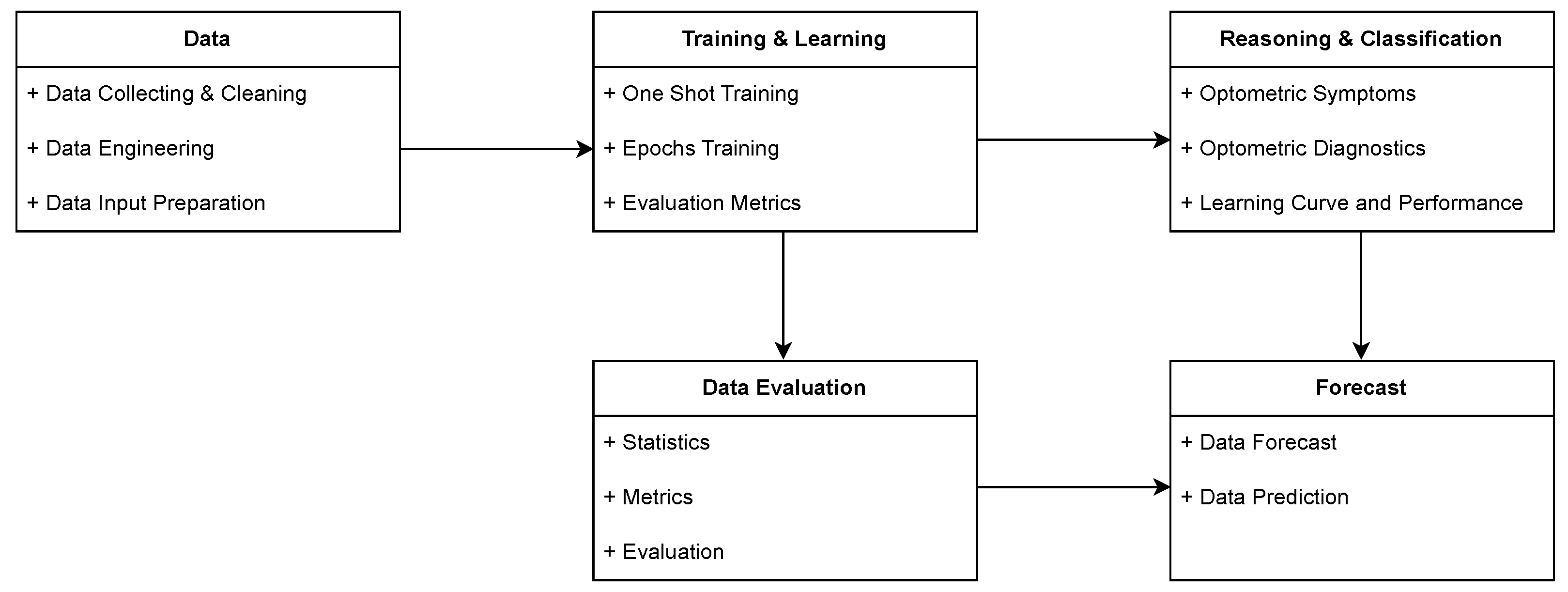
The initial stage of the process encompasses data collection, cleaning, engineering, and input preparation to ensure high-quality input for ML and AI models. Optometry-related academic articles published between 2000 and 2023 were retrieved from the Web of Science database. To refine the dataset, all non-essential metadata, such as DOI, webpage links, and author information, were removed. Subsequently, the dataset underwent preprocessing to optimize its structure for ML algorithms. This step ensured that the raw optometric data was adequately processed and formatted to enhance its suitability for subsequent ML and AI analyses.

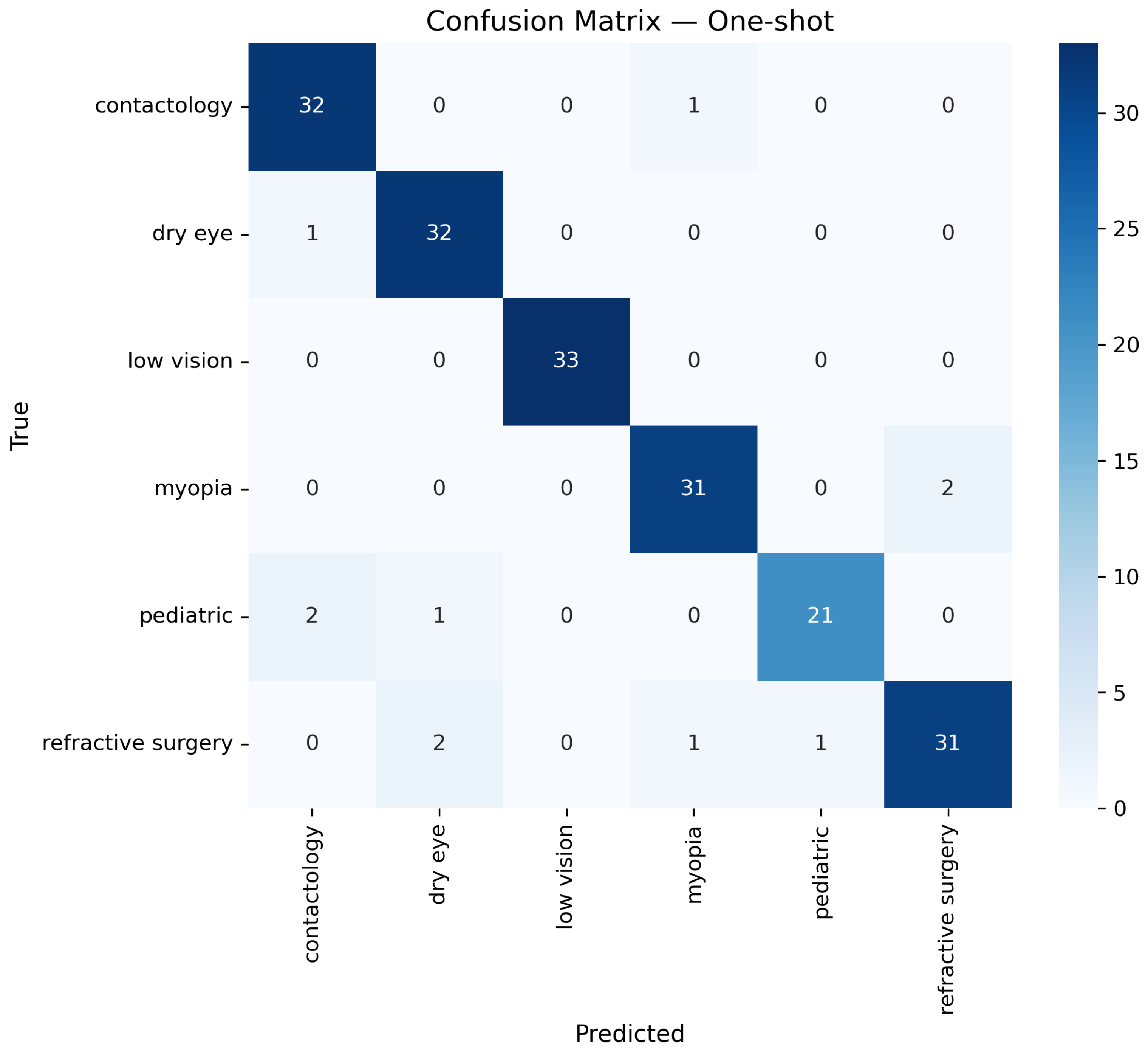
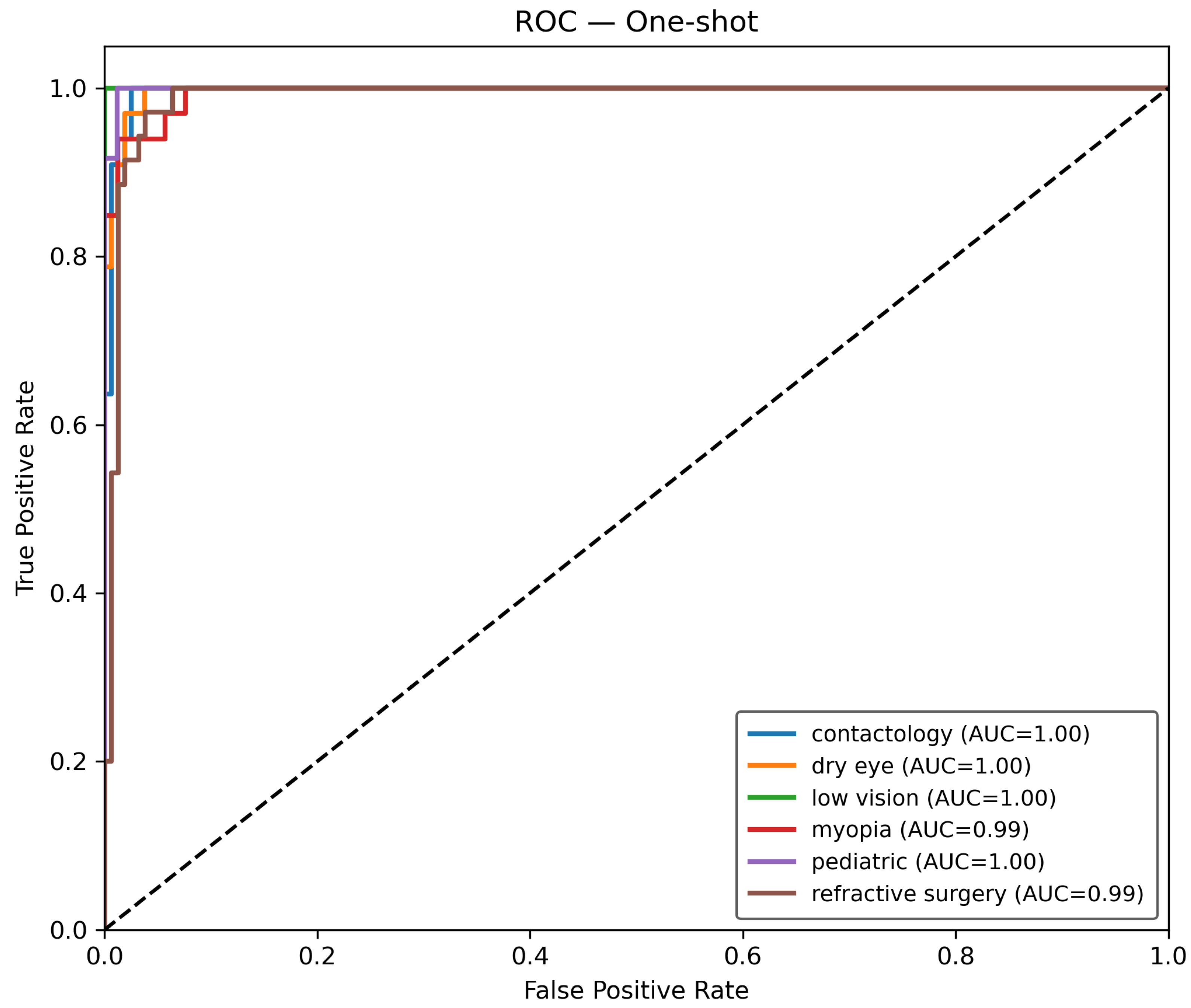
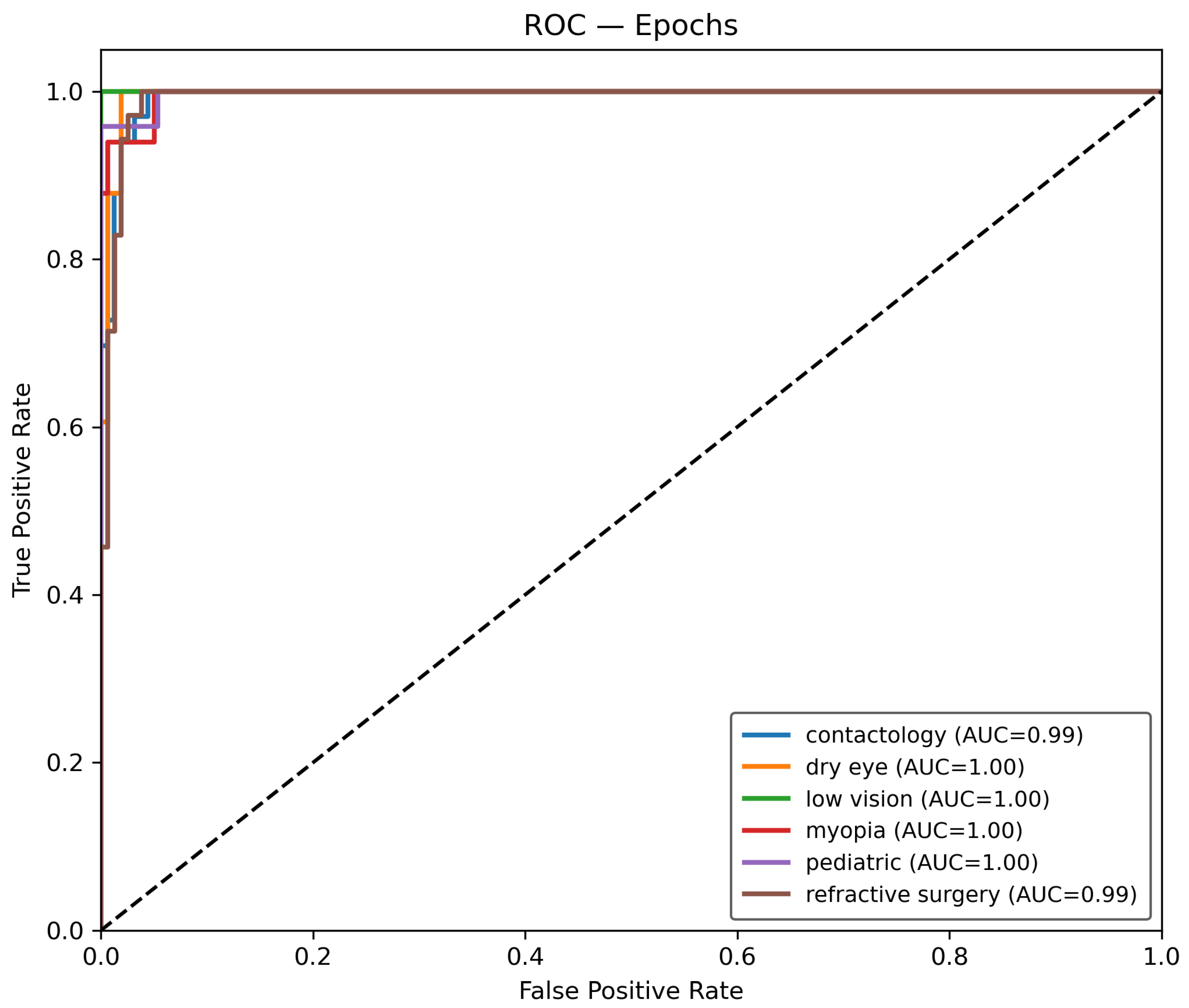
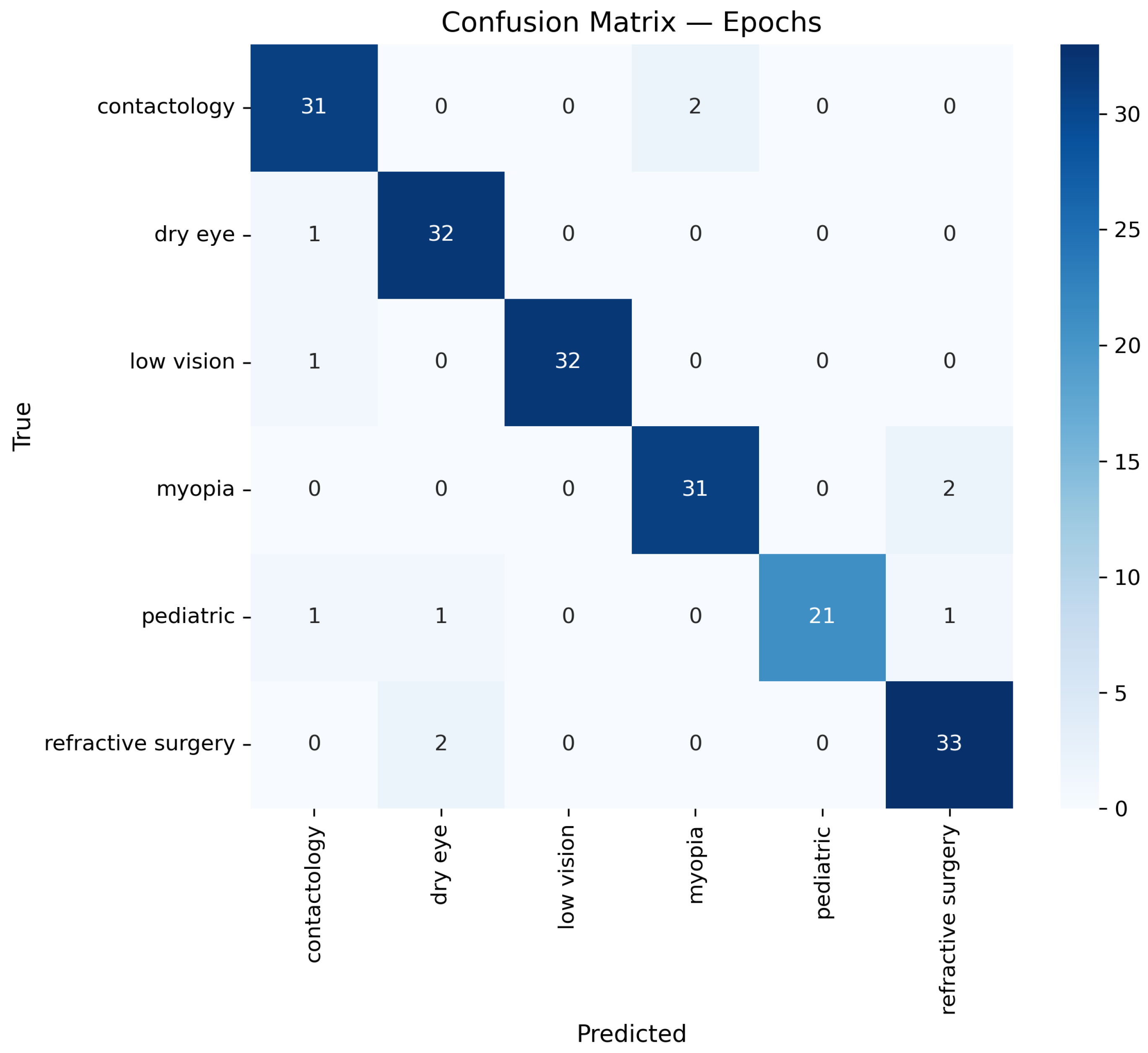
Once the data is prepared, it is used in the O-RF ML workflow comprising one-shot training and epoch-based training. One-shot training refers to models trained with minimal supervised labeled data. Regarding the epoch training, it involved iterative learning over multiple cycles, allowing models to refine their weights and optimize performance. After these two different approaches, the evaluation metrics were computed to ensure the reliability and validity of the models by assessing classification accuracy, precision, recall, F1-score, and AUC-ROC.

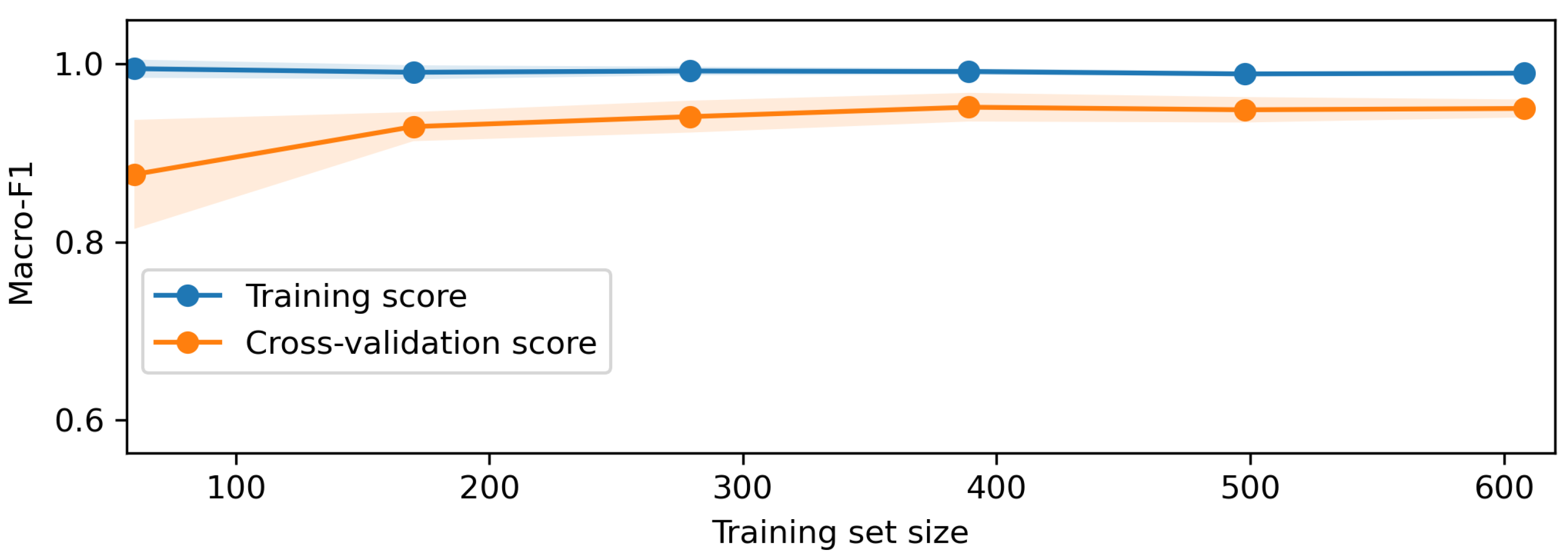
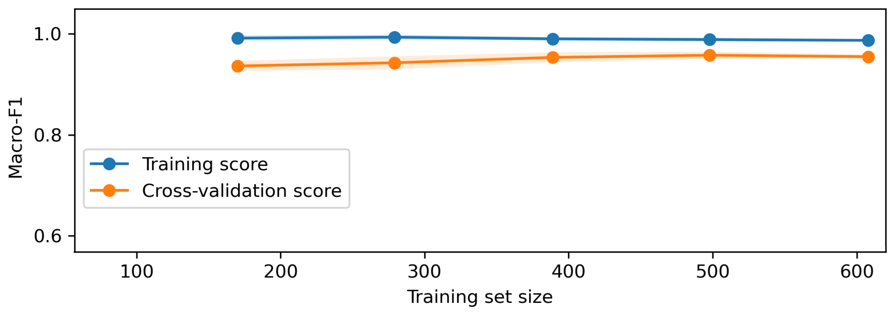
The AI block focuses on the optometric data recognition, diagnostic inference, and learning curve assessment. The optometric data extraction involves recognizing features from the raw data using NLP capabilities. This optometric data diagnostic leverage the trained AI models to provide automated assessments. The learning curve and performance analysis provide an overview of the model’s ability and capacity in the performance of the diagnosis tasks.

The data science module underpins the entire framework, integrating statistical methodologies, metric analysis, and evaluation techniques. These quantitative methods ensure that AI models remain interpretable and statistically valid, fostering transparency and trust for data forecasts and diagnoses.

The final component of the framework focuses on data forecasting and prediction for optometric outcomes, employing the ARIMA model. The ARIMA model was selected as the primary forecasting technique due to its well-established reliability in time-series analysis and its transparent, interpretable nature compared to deep learning approaches. ARIMA enables the model to extrapolate trends and patterns from historical data, facilitating the prediction of future optometric outcomes. The selection of ARIMA was also driven by its widespread adoption in the medical field due to its robustness in time-series analysis and forecasting applications. Its proven effectiveness in capturing temporal dependencies and trends makes it a suitable choice for predictive modeling in optometric diagnostics. Furthermore, ref. [9] demonstrated ARIMA’s effectiveness in predicting disease prevalence and research trends in healthcare applications, including neuroscience and ophthalmology.

2.1. Data

For the development of AI software, the random forest model was selected as the primary ML architecture because of its robustness in classification tasks. The random forest model is not pre-trained, and because so, it requires training from scratch. To address this, the model was trained by one-shot and epochs, using a dataset comprising 32,485 academic articles from the field of optometry, sourced from the Web of Science and spanning from 2000 to 2023. These academic articles used for training were all peer-reviewed, ensuring the training data quality.

Table 1. Collected optometry papers from Web of Science [15].

	Number of		Number of		Number of		Number of		Number of
Year	Articles	Year	Articles	Year	Articles	Year	Articles	Year	Articles
2000	457	2005	576	2010	1392	2015	1318	2020	2445
2001	427	2006	653	2011	1133	2016	1388	2021	2801
2002	418	2007	721	2012	1175	2017	1477	2022	2916
2003	481	2008	815	2013	1555	2018	1654	2023	2800
2004	562	2009	907	2014	1564	2019	1990

presents the number of academic articles published in each year.

To avoid data imbalance in the AI model, ML supervised training was carefully conducted with a similar number of articles for each labeled dataset, and the ML metrics were closely monitored. From the entire dataset, 951 articles were used in supervised training to enhance the optometry knowledge of the model. The classification framework utilizes an O-RF model, trained to differentiate among six optometric categories: Contactology, Dry Eye, Low Vision, Myopia, Pediatrics, and Refractive Surgery. The model assigns probabilities to each class based on a combination of decision trees, leveraging feature importance weighting to enhance classification reliability.

2.2. O-RF Mathematical Formulation

The O-RF model has undergone one-shot and epoch training. In order to do so, it is necessary to train O-RF in identifying and diagnosing each type of data within the entire dataset. Regarding this, a supervised training method was chosen, where data is labeled in accordance with its characteristics. The number of data classified under each label is presented in

Table 2. Supervised Training Data [15].

Label	Number
Contactology	163
Dry Eye	164
Low Vision	164
Myopia	163
Pediatric	121
Refractive Surgery	176

.

Having the dataset and the training data available, the next step is to perform the mathematical formulation that transforms the Table 1 and Table 2 raw text data into a numerical feature representation using the Term Frequency-Inverse Document Frequency (TF-IDF) method. This process is essential for converting unstructured textual data into a structured format suitable for machine learning models.

For any given document $d_i$ and a term $t_j$, let $f_{ij}$ denote the frequency of term $t_j$ in document $d_i$. The normalized term frequency is defined as:

$$\mathrm{tf}(t_j,d_i)={\displaystyle \frac{f_{ij}}{{\sum }_{k=1}^d{f}_{ik}}}$$

(1)

In Equation (1), numerator $f_{ij}$ represents the raw count of term $t_j$ in document $d_i$, and the denominator sums the counts of all d terms in $d_i$, thus normalizing the term frequency relative to the document length. The inverse document frequency quantifies the importance of the term $t_j$ across the entire corpus $\mathcal{D}$ consisting of N documents.

$$\mathrm{idf}\left(t_j\right)=log\left({\displaystyle \frac{N}{1+\left|\right\{d_i\in \mathcal{D}:t_j\in d_i\left\}\right|}}\right)$$

(2)

In Equation (2), N is the total number of documents, and $\left|\right\{d_i\in \mathcal{D}:t_j\in d_i\left\}\right|$ denotes the number of documents in which term $t_j$ appears. The addition of 1 in the denominator prevents division by zero, ensuring numerical stability.

The TF-IDF weight for term $t_j$ in document $d_i$ is the product of the normalized term frequency and the inverse document frequency.

$$w_{ij}=\mathrm{tf}(t_j,d_i)·\mathrm{idf}\left(t_j\right)$$

(3)

Equation (3) combines local term frequency with global inverse document frequency, resulting in a weight $w_{ij}$ that reflects both the importance of $t_j$ in $d_i$ and its rarity across the corpus.

With the TF-IDF weights computed, each document $d_i$ can be represented as a d-dimensional feature vector.

$$x_i=\left[\begin{array}{c}{w}_{i1}\\ w_{i2}\\ ⋮\\ w_{id}\end{array}\right]\in {\mathbb{R}}^d$$

(4)

In Equation (4), ${\mathbf{x}}_i$ encapsulates the TF-IDF weights for all d terms in the vocabulary, where each $w_{ij}$ is defined in (3).

The overall transformation from raw text to a numerical feature vector is encapsulated by the mapping function T.

$$T\left(d_i\right)={\left({\displaystyle \frac{f_{ij}}{{\sum }_{k=1}^d{f}_{ik}}}·log\left({\displaystyle \frac{N}{1+\left|\right\{d\in \mathcal{D}:t_j\in d\left\}\right|}}\right)\right)}_{j=1}^d$$

(5)

Equation (5) represents the complete process for converting a document $d_i$ into its corresponding TF-IDF feature vector, where the computation for each term $t_j$ is performed as described in the previous steps.

Despite a careful data labeling process to avoid class imbalance, an automated process to deal specifically with detected imbalance in the data was created for O-RF. The process to deal with this imbalance can be mathematically described. Let ${\mathcal{X}}_{\min }={\left\{{\mathbf{x}}_i\right\}}_{i=1}^{N_{\min }}$ be the set of samples belonging to the minority class, where $N_{\min }$ is the number of minority samples. To address class imbalance, the Synthetic Minority Oversampling Technique (SMOTE) is employed to generate synthetic samples by interpolating between existing minority samples and their nearest neighbors in the feature space.

For each minority sample ${\mathbf{x}}_i\in {\mathcal{X}}_{\min }$, the k nearest neighbors ${\left\{{\mathbf{x}}_i^{\left(j\right)}\right\}}_{j=1}^k$ are identified, typically using the Euclidean distance. Then, for each selected neighbor ${\mathbf{x}}_i^{\left(j\right)}$, a synthetic sample $\tilde{\mathbf{x}}$ is generated using Equation (6).

$$\tilde{\mathbf{x}}={\mathbf{x}}_i+\lambda \left({\mathbf{x}}_i^{\left(j\right)}-{\mathbf{x}}_i\right),\lambda \sim \mathcal{U}(0,1)$$

(6)

In Equation (6), $\lambda$ is a random variable drawn from a uniform distribution $\mathcal{U}(0,1)$. This ensures that the synthetic sample $\tilde{\mathbf{x}}$ lies on the line segment between ${\mathbf{x}}_i$ and ${\mathbf{x}}_i^{\left(j\right)}$. If an oversampling ratio $\alpha$ is defined (with, for instance, $\alpha =1$ implying equal numbers of minority and majority class samples), the number of synthetic samples $N_{\mathrm{synthetic}}$ required to achieve the desired balance.

$$N_{\mathrm{synthetic}}=\alpha ·N_{\min }-N_{\min }$$

(7)

Equation (7) determines the total number of new synthetic samples to be generated so that the final minority class count becomes $\alpha ·N_{\min }$.

Generating synthetic samples via interpolation as shown in (6), ensuring that new samples reside within the local neighborhood of existing minority instances. Adjusting the overall class distribution according to the desired oversampling ratio defined in (7). This mathematical framework allows the model to learn from a more balanced dataset if a data imbalance is detected, thus mitigating biases introduced by the original class imbalance.

The O-RF uses a derivation of the original RF since it relies on training exclusively with optometry academic articles. For the O-RF model, let $\mathcal{D}={\left\{({\mathbf{x}}_i,y_i)\right\}}_{i=1}^N$ denote the training dataset, where ${\mathbf{x}}_i\in {\mathbb{R}}^d$ is the feature vector and $y_i\in \{1,2,\dots ,C\}$ is the class label of the i-th sample. The O-RF is an ensemble method that aggregates predictions from T decision trees to improve the classification.

For each tree t ($t=1,\dots ,T$), a bootstrap sample ${\mathcal{D}}_t$ is drawn from $\mathcal{D}$ with replacement. At each node of tree t, a random subset of features is selected from the full set of d features. This subset is given by Equation (8) where m is a hyperparameter such that $m\ll d$.

$$F_t\subset \{1,2,\dots ,d\},\left|F_t\right|=m$$

(8)

At each node, the optimal split is determined by selecting the feature $j\in F_t$ and a threshold $\theta$ that minimizes an impurity measure $\mathcal{I}$. The choice is the Gini impurity because it measures how often a randomly chosen element would be incorrectly labeled if it were labeled randomly and independently. Regarding this, the Gini impurity is defined for a region R as Equation (9).

$$G\left(R\right)=1-\sum _{c=1}^{C}p{\left(c\right|R)}^2$$

(9)

In Equation (9), the $p\left(c\right|R)$ is the proportion of samples in R that belong to class c. The optimal split $(j^{*},{\theta }^{*})$ is obtained by solving Equation (10).

$$(j^{*},{\theta }^{*})=arg\underset{j\in F_t,\theta }{min}\left[{\displaystyle \frac{|R_{\mathrm{left}}|}{\left|R\right|}}\mathcal{I}\left(R_{\mathrm{left}}\right)+{\displaystyle \frac{|R_{\mathrm{right}}|}{\left|R\right|}}\mathcal{I}\left(R_{\mathrm{right}}\right)\right]$$

(10)

where $R_{\mathrm{left}}$ and $R_{\mathrm{right}}$ are the two regions created by splitting R with the candidate $(j,\theta )$, and $\left|R\right|$ denotes the number of samples in region R.

Each decision tree $h_t$ partitions the feature space into disjoint regions ${\left\{R_{tc}\right\}}_{c=1}^C$, where each region $R_{tc}$ is associated with class c. The prediction of tree t for a new sample $\mathbf{x}$ is calculated per Equation (11).

$$h_t\left(\mathbf{x}\right)=\sum _{c=1}^{C}c{\mathbf{1}}_{\{\mathbf{x}\in R_{tc}\}}$$

(11)

where ${\mathbf{1}}_{\left\{·\right\}}$ is the indicator function that equals 1 if $\mathbf{x}$ belongs to region $R_{tc}$ and 0 otherwise.

The final prediction $\widehat{y}$ of the O-RF is obtained by aggregating the predictions of all T trees via majority voting using Equation (12), where mode denotes the most frequently occurring class among the individual tree predictions.

$$\widehat{y}=mode{\left\{h_t\left(\mathbf{x}\right)\right\}}_{t=1}^T$$

(12)

One of the key features for every ML model is the chosen hyperparameters since they are crucial to the model tuning and outcome. Let the hyperparameter configuration be denoted as per Equation (13).

$$\theta =({\theta }_1,{\theta }_2,\dots ,{\theta }_k)\in \Theta$$

(13)

where $\Theta$ represents the discrete search space formed by the Cartesian product of the possible values for each hyperparameter.

The goal of grid search is to identify the optimal configuration ${\theta }^{*}$ that maximizes the performance of the model, as measured by a cross-validation metric. This is mathematically formulated in Equation (14).

$${\theta }^{*}=arg\underset{\theta \in \Theta }{max}\mathrm{CV}\left(\theta \right)$$

(14)

where $\mathrm{CV}\left(\theta \right)$ denotes the cross-validation score obtained for configuration $\theta$. In a K-fold cross-validation framework, the cross-validation score is calculated as the average performance across all the K folds per Equation (15).

$$\mathrm{CV}\left(\theta \right)={\displaystyle \frac{1}{K}}\sum _{i=1}^K{\mathrm{score}}_i\left(\theta \right)$$

(15)

where ${\mathrm{score}}_i\left(\theta \right)$ is the performance metric measured on the i-th fold using the hyperparameter configuration $\theta$. The optimized hyperparameters for the O-RF model are presented in

Table 3. Hyperparameters for the one-shot O-RF and epoch O-RF pipelines.

Stage	Hyperparameter	Description	Values
TF-IDF	tfidf__max_features	Vocabulary size	2000, 5000
TF-IDF	tfidf__ngram_range	N-grams included	(1,1), (1,2)
SMOTE	smote__k_neighbors	Nearest neighbors for synthesis	3, 5
O-RF	rf__n_estimators	Number of trees	300, 600
O-RF	rf__max_depth	Maximum tree depth	10, 20
O-RF	rf__min_samples_leaf	Minimum samples per leaf	2, 5
O-RF	rf__max_features	Features considered at each split	sqrt
O-RF	rf__class_weight	Class weighting	None, balanced_subsample
TF-IDF	tfidf__max_features	Vocabulary size	3000, 6000
TF-IDF	tfidf__ngram_range	N-grams included	(1,1), (1,2)
TF-IDF	tfidf__min_df	Minimum document frequency	2, 3
TF-IDF	tfidf__max_df	Maximum document frequency	0.85, 0.90
TF-IDF	tfidf__sublinear_tf	Sublinear TF scaling	True
LR	clf__C	Inverse regularization strength	0.25, 0.50, 1.00
LR	clf__class_weight	Class weighting	None, balanced
CV	StratifiedKFold	5-fold CV with shuffling	n_splits = 5, shuffle = True, random_state = 42
SMOTE	random_state	Reproducibility	42
RF	random_state, n_jobs	Seed and parallelism	42, −1
LR	solver, multi_class, max_iter, n_jobs, random_state	Logistic regression configuration	saga, ovr, 2000, −1, 42

.

The last step in to compute the performance metrics for the O-RF model. In order to assess all the relevant metrics, let us consider N to be the total number of samples in the test set. For each sample i, let $y_i$ denote the true label and ${\widehat{y}}_i$ the predicted label. The first performance metric calculated per Equation (16) is accuracy, which measures the proportion of correctly classified samples, or in other terms, accuracy gives how often the model is correct.

$$\mathrm{Accuracy}={\displaystyle \frac{1}{N}}\sum _{i=1}^N\mathbf{1}\left({\widehat{y}}_i=y_i\right)$$

(16)

In Equation (16), $\mathbf{1}\left(·\right)$ is a binary indicator function, which is 1 when the condition is true and 0 otherwise.

Another important indicator in ML models evaluation is precision. The precision metric, given in Equation (17), provides insights into the model’s ability to correctly predict positive instances while minimizing the risk of false predictions.

$${\mathrm{Precision}}_c={\displaystyle \frac{T{P}_c}{T{P}_c+F{P}_c}}$$

(17)

where for any specific class c, $T{P}_c$ is the number of true positives, $F{P}_c$ is the number of false positives, and $F{N}_c$ is the number of false negatives.

Recall, also known as sensitivity or true positive rate, is also another important metric in classification that emphasizes the model’s ability to identify all relevant instances. Recall, given by Equation (18), measures the proportion of actual positive cases correctly identified by the model.

$${\mathrm{Recall}}_c={\displaystyle \frac{T{P}_c}{T{P}_c+F{N}_c}}$$

(18)

The F1-score for class c, calculated by Equation (19), represents the harmonic mean of precision and recall.

$$F{1}_c={\displaystyle \frac{2·{\mathrm{Precision}}_c·{\mathrm{Recall}}_c}{{\mathrm{Precision}}_c+{\mathrm{Recall}}_c}}$$

(19)

The Receiver Operating Characteristic (ROC) curve is defined by the true positive rate (TPR) given by Equation (20), and the false positive rate (FPR) given by Equation (21) for various threshold values t. For class c, these are computed as:

$${\mathrm{TPR}}_c\left(t\right)={\displaystyle \frac{T{P}_c\left(t\right)}{T{P}_c\left(t\right)+F{N}_c\left(t\right)}}$$

(20)

$${\mathrm{FPR}}_c\left(t\right)={\displaystyle \frac{F{P}_c\left(t\right)}{F{P}_c\left(t\right)+T{N}_c\left(t\right)}}$$

(21)

where $T{N}_c\left(t\right)$ is the number of true negatives for class c at threshold t. The Area Under the Curve (AUC) for class c is then given by Equation (22).

$${\mathrm{AUC}}_c={\int }_0^1{\mathrm{TPR}}_c\left({\mathrm{FPR}}_c^{-1}\left(x\right)\right)dx$$

(22)

which represents the probability that a randomly chosen positive instance is ranked higher than a randomly chosen negative instance.

Another crucial performance metric is specificity, also known as the true negative rate (TNR). Specificity measures the model’s ability to correctly identify negative instances, ensuring that the model minimizes false positives. This metric is defined in Equation (23).

$${\mathrm{Specificity}}_c={\displaystyle \frac{T{N}_c}{T{N}_c+F{P}_c}}$$

(23)

A high specificity value indicates that the model is effective in recognizing negative instances while reducing the likelihood of false positives.

2.3. Forecast

The ARIMA model is a classical time series forecasting method that captures temporal dependencies in the data through autoregressive (AR) and moving average (MA) components, combined with differencing to induce stationarity. An ARIMA model is denoted as ARIMA($p,d,q$), where p is the order of the autoregressive part, d is the degree of differencing, and q is the order of the moving average part.

Regarding Equation (24), $y_t$ denotes the observed time series at time t, B is the backshift operator defined by $B{y}_t=y_{t-1}$, ${\varphi }_1,{\varphi }_2$ are the autoregressive coefficients, ${\theta }_1$ is the moving average coefficient, and ${ϵ}_t$ is a white noise error term.

$$\left(1-{\varphi }_{1}B-{\varphi }_2{B}^2\right)(1-B)y_t=\left(1+{\theta }_{1}B\right){ϵ}_t$$

(24)

Once the model is fitted to the historical data, the h-step-ahead forecast is computed as the conditional expectation using Equation (25).

$${\widehat{y}}_{T+h}=E\left(y_{T+h}\mid {\mathcal{F}}_T\right)$$

(25)

where T is the last observed time point and ${\mathcal{F}}_T$ represents the information set up to time T. The term $y_{T+h}$ corresponds to $\widehat{y}$ from Equation (12), connecting the ML to the forecast model.

With this feature, the ARIMA model examines the time-series data to predict future trends by leveraging historical patterns. This approach aids in understanding how specific categories change over time and in forecasting future developments in optometry. To facilitate this transformation, dimensionality reduction techniques can be employed to process embedding $y_{T+h}$, extracting the most relevant features that highlight key data trends. This step of quantification is essential for effectively capturing the core aspects of the research focus within the high-dimensional space of O-RF embeddings.

2.4. O-RF Tuning

With the O-RF trained model fine-tuned for optometry outputs, the developed model can be used to automatically classify any type of information within the dataset. This is performed by letting $H:{\mathbb{R}}^d\to \{1,2,\dots ,C\}$ be the classification function derived from the trained model. For any new input feature vector $\mathbf{x}\in {\mathbb{R}}^d$, the predicted class label is given by Equation (26).

$$\widehat{y}=H\left(\mathbf{x}\right)$$

(26)

For a dataset consisting of N samples $\mathbf{X}=\{{\mathbf{x}}_1,{\mathbf{x}}_2,\dots ,{\mathbf{x}}_N\}$, the prediction for the entire dataset is:

$$\widehat{Y}=\{H\left({\mathbf{x}}_1\right),H\left({\mathbf{x}}_2\right),\dots ,H\left({\mathbf{x}}_N\right)\}$$

(27)

In Equations (26) and (27), $H\left(·\right)$ encapsulates the ensemble decision process, and $\widehat{Y}$ represents the predicted class label(s).

The AI learning curve can be built to illustrate the relationship between the model performance and the training data. Let $n\in \{n_1,n_2,\dots ,n_L\}$ represent different training set. The training performance can be defined as per Equation (28).

$${\mathrm{Score}}_{\mathrm{train}}\left(n\right)={\displaystyle \frac{1}{n}}\sum _{i=1}^n\mathbf{1}\left(H\left({\mathbf{x}}_i\right)=y_i\right)$$

(28)

The corresponding validation performance, computed via K-fold cross-validation, is given by Equation (29).

$${\mathrm{Score}}_{\mathrm{val}}\left(n\right)={\displaystyle \frac{1}{K}}\sum _{j=1}^K{\mathrm{score}}_j\left(n\right)$$

(29)

Here, ${\mathrm{score}}_j\left(n\right)$ is the performance metric computed on the j-th validation fold using a subset of n training samples.

3. Results

3.1. O-RF Metrics

Both the one-shot and epoch-based O-RF models were compiled into versions occupying less than 1 GB of storage. Training the full pipeline required under one hour, and inference consistently produced results within five seconds on a low-end computer without GPU acceleration. These characteristics indicate that the proposed framework is both efficient and practical for deployment on low-resource hardware while retaining state-of-the-art classification performance.

The metrics for the O-RF model with one-shot training, meaning that the model has only one pass through all the data, for the various classes are summarized in

Table 4. Performance indicators from the O-RF model by one-shot training.

Metric|Label	Contactology	Low Vision	Refractive Surgery	Pediatric	Myopia	Dry Eye
F1-Score	94.12%	100%	91.18%	91.30%	93.94%	94.12%
AUC	99.62%	100%	98.90%	99.90%	99.48%	99.65%
Recall	96.97%	100%	88.57%	87.50%	93.94%	96.97%
Specificity	98.10%	100%	98.72%	99.40%	98.73%	98.10%
Overall Precision:	94.37%
Overall Accuracy:	94.24%

, indicating an average F1-score of 94.11%, an almost perfect Area Under the Curve (AUC) score of 99.59%, a precision of 94.37%, and an accuracy of 94.24%.

In ML a confusion matrix provides a structured representation of classification performance, particularly in supervised learning. Each row in the matrix corresponds to instances assigned to a predicted class, while each column represents the actual class labels. The confusion matrix is a crucial tool for evaluating metrics such as recall, precision, and accuracy, offering deeper insights into the model’s strengths and areas requiring improvement.

The confusion matrix presented in Figure 2 provides a detailed breakdown of classification performance for the trained O-RF model. The diagonal values of 36, 30, 42, 30, 23, and 45 represent the number of correctly classified instances for Contactology, Dry Eye, Low Vision, Myopia, Pediatric, and Refractive Surgery, respectively. These figures indicate a high classification accuracy across most categories, reinforcing the model’s robustness in distinguishing between different optometric conditions.

However, the off-diagonal entries highlight instances of misclassification, which merit further analysis. Notably, Dry Eye was misclassified as Contactology in one instance, Myopia was misclassified as Pediatric in one case, and Pediatric was misclassified as Myopia and Refractive Surgery in two cases. These errors suggest that certain classes share overlapping feature spaces, potentially leading to classification ambiguity.

The Receiver Operating Characteristic (ROC) curve given by Figure 3 provides a graphical representation of the O-RF model’s classification capability across different optometry-related categories. The AUC values summarized in Table 4 confirm the model’s performance, with all six classes achieving an AUC close to 1.00. This indicates that the O-RF model demonstrates flawless classification between positive and negative instances. The ROC curves for each class are expected to closely align with the upper-left boundary of the ROC space, indicating that the model consistently minimizes false positives while maximizing true positive identification. Such uniformity in performance illustrates the robustness and reliability of the O-RF model, making it a highly effective tool for clinical applications where precise and dependable classification is crucial. The ability to consistently achieve an AUC close to 1.00 across diverse diagnostic categories suggests that this model can play a vital role in automated decision-making systems within optometry and related medical fields, contributing to enhanced diagnostic accuracy and improved patient outcomes.

The above metrics were derived using a one-shot training approach, where the entire dataset is fed to the model in a single exposure, enabling it to adjust its weights based on this solitary pass. This technique offers advantages in terms of computational efficiency and simplicity, which took about 38 min to run on an eight-core i5-10210U CPU at 1.60 GHz–2.11 GHz; however, in theory it may lead to suboptimal performance because of the single data passage. The primary limitation of one-shot training is its potential inability to capture the full complexity of the data, which can result in non-optimized models.

Conversely, a more iterative approach involves training the model over multiple epochs, where the dataset is processed several times. This method allows, in theory, the model to gradually refine its parameters and improve its ability to discern intricate patterns through progressive learning. Each epoch represents a complete pass through the dataset, with subsequent updates to the model’s weights. Although this process is computationally more demanding and time-intensive compared to one-shot training, which took about 38 times the time to fully run compared with the one-shot, it can in theory yield superior performance, particularly when dealing with large and/or complex datasets. By facilitating repeated exposure to the data, training over multiple epochs enhances the model’s capacity to generalize, leading to more robust and accurate predictions.

Regarding this, the O-RF model has undergone training for 500 epochs using the same dataset and supervised learning methodology. The performance metrics for epoch-trained O-RF are given in

Table 5. Performance indicators from the O-RF model by epoch training pipeline.

Metric|Label	Contactology	Low Vision	Refractive Surgery	Pediatric	Myopia	Dry Eye
F1-Score	92.54%	98.46%	92.96%	93.33%	93.93%	94.12%
AUC	99.44%	100%	99.29%	99.78%	99.65%	99.60%
Recall	93.94%	96.97%	94.29%	87.50%	93.94%	96.97%
Specificity	98.10%	100%	98.08%	100%	98.73%	98.10%
Overall Precision:	94.70%
Overall Accuracy:	94.24%

. With the epoch training methodology, it is possible to perceive an improvement in all indicators and across all labels when compared to the one-shot method.

The ROC curve, depicted in Figure 4, provides a robust evaluation of the O-RF model’s discriminative ability across different optometry classes. The AUC values remain consistently very close to 100% for all classes, demonstrating that the model achieves perfect separation between positive and negative cases. This optimal classification performance suggests that the model successfully differentiates between conditions without ambiguity, effectively balancing sensitivity and specificity across all categories.

The high specificity values, as seen in Table 5, further reinforce the model’s ability to minimize false positives. Notably, all classes achieve specificity values near 100%, confirming an exceptionally low rate of misclassification. These results are particularly critical in clinical applications, where high specificity is essential to prevent unnecessary interventions caused by false positive classifications.

While the recall values exhibit slight variations, the model maintains robust sensitivity across all classes. Low Vision and Dry Eye achieve the highest recall with 97%, ensuring that close to all true positive instances are correctly identified. However, Pediatric with 87.50% shows slightly lower recall values, indicating that while the model is effective at detecting these conditions, there may be a small fraction of missed cases. This aligns with the F1-scores of these classes, 93.33% for Pediatric and 93.93% for Myopia, suggesting a minor trade-off between precision and recall in these categories. Despite this, the overall precision classification with 94.70% and accuracy with 94.24% reflect the model’s reliability in practical decision-making scenarios.

The consistent AUC values across all classes highlight the robustness of the O-RF model in handling complex classification tasks. The near-perfect precision-recall balance and the model’s ability to maintain high F1-scores across all categories emphasize its utility for clinical implementation. The strong generalizability of the model, as evidenced by its exceptional specificity and recall across multiple epochs, positions it as a highly effective tool for optometric diagnostics, where both sensitivity and specificity are paramount to ensuring accurate clinical outcomes. Both one-shot and epoch O-RF achieve exceptionally high accuracy and AUC scores; the high metrics raised concerns about the potential risk of overfitting due to repeated training cycles on the same dataset. To mitigate this, k-fold cross-validation (k = 10) was applied to assess the model’s robustness across different subsets of the dataset. Additionally, a hold-out validation set (20% of the data) was used to evaluate generalization performance. The results indicate that the model maintains high performance on unseen data, with minimal degradation in accuracy of less than 1%.

The confusion matrix in Figure 5 summarizes the classification behavior of the epoch training pipeline across the six optometry classes. Correct predictions are concentrated on the diagonal and remain high in every class: Contactology 31/33, Dry Eye 32/33, Low Vision 32/33, Myopia 31/33, Pediatric 21/24, and Refractive Surgery 33/35. Off-diagonal counts are small and reveal a few systematic confusions.

The most frequent errors are: Contactology mislabelled as Myopia (2 cases), Dry Eye mislabelled as Contactology (1), Low Vision mislabelled as Contactology (1), Myopia mislabelled as Refractive Surgery (2), Pediatric mislabelled as Contactology, Dry Eye and Refractive Surgery (1 each), and Refractive Surgery mislabelled as Dry Eye (2). These patterns are consistent with the per-class recall reported in Table 5: Pediatric shows the lowest recall at 87.50% (21/24), followed by Contactology and Myopia at 93.94% (31/33 each), while Dry Eye, and Low Vision reach 96.97% (32/33), and Refractive Surgery attains 94.29% (33/35). Specificity is high across the board, with Low Vision and Pediatric at 100% and the remaining classes above 98%, matching the table.

Overall performance remains strong, with overall accuracy of 94.24% and overall precision of 94.70% (Table 5). The error structure indicates occasional overlap between semantically related categories, notably Myopia and Refractive Surgery, and a small amount of leakage from Pediatric into adjacent categories, yet the model preserves a low false positive rate and reliable discrimination for clinical decision support.

3.2. Forecast

Regarding the data forecast,

Table 6. ARIMA forecasted data.

Data Label|Year	2025	2026	2027	2028	2029	2030
Contactology	64	66	64	66	64	66
Dry Eye	84	80	83	82	81	82
Low Vision	81	81	81	81	81	81
Myopia	159	164	160	160	161	161
Pediatric	393	401	398	398	399	398
Refractive Surgery	79	74	75	76	75	75

presents the projected academic research trends for the prevalence of various optometry-related data from 2025 to 2030. These forecasts were generated using an ARIMA model, providing insights into how the data might evolve over time.

The projections reveal distinct patterns across different categories. Pediatric-related research is expected to maintain the highest prevalence, with a steady increase from 393 in 2025 to 401 in 2026, followed by a stabilization around 398–399 in subsequent years. This consistent upward trend suggests sustained growth in pediatric optometry.

Similarly, the Myopia class demonstrates relative stability, with 159 data entries in 2025, peaking at 164 in 2026, and then maintaining values around 160–161 through 2030. This indicates a continued focus on Myopia, likely due to its increasing global impact.

On the other hand, Dry Eye shows minor fluctuations, with a projected decline from 84 in 2025 to 80 in 2026, followed by a modest recovery to 83 in 2027, and then a slight stabilization near 81–82. This suggests periodic variations rather than a sustained growth or decline.

Low Vision-related publications remain completely stable, with a consistent forecast of 81 data entries per year throughout the entire analyzed period, implying a steady level without significant expected growth or decline.

Contactology and Refractive Surgery display alternating patterns, with Contactology fluctuating between 64 and 66 data entries and Refractive Surgery initially declining from 79 in 2025 to 74 in 2026 before stabilizing around 75–76 in later years. This suggests a cyclical behavior rather than a steady upward or downward trajectory.

Overall, these ARIMA-based forecasts indicate that while some optometry subfields, such as Pediatric and Myopia, are likely to remain dominant, others, like Refractive Surgery and Dry Eye, may experience more variability in the data trends. These projections can serve as a valuable guide for researchers and policymakers, helping to anticipate emerging trends and allocate resources accordingly.

3.3. O-RF Performance

The integration of AI in optometry classification tasks can potentially provide significant advancements in diagnostic accuracy and decision-making processes. The effectiveness of an AI-based model is often assessed using learning curves and performance trends, providing insights into model generalization, stability, and reliability. The AI-based classification framework presented leverages the combination of two distinct training strategies within the Random Forest architecture: the O-RF one-shot trained, which was trained on a single batch of labeled data, enabling rapid learning with high initial accuracy, and the O-RF epoch-trained, which is refined iteratively over multiple training epochs, enhancing generalization and adaptability to unseen data. Figure 6 and Figure 7 illustrate the learning progression and classification performance for both the one-shot and epoch O-RF models, highlighting their adaptability to increasing training data and their long-term consistency in AI-driven classification tasks. Figure 6 and Figure 7 illustrate the learning curves using Macro-F1, which is the appropriate metric for the analyzed multi-class dataset because it averages performance across classes rather than letting majority classes dominate. Curves were computed with stratified cross-validation on a leakage-safe pipeline in which TF-IDF and SMOTE are fitted only inside the training folds.

For the one-shot configuration, the training curve sits close to 0.99 across all sampling levels, while the cross-validation curve climbs steadily from roughly 0.88 at the smallest training size to approximately 0.95 at the largest. The gap between the curves shrinks as more data are used, from about 0.12 at the smallest size to about 0.05 at the largest. The shaded uncertainty band around the validation curve contracts with sample size, which indicates decreasing variance across folds. Regarding this, it is safe to say that the developed model does not present overfitting, since a model that is genuinely overfitting shows the opposite pattern: a training curve near perfection coupled with a validation curve that stagnates or degrades as additional training data are added, often with widening uncertainty. None of those signatures appear here. Instead, the validation curve approaches the training curve and stabilizes at a high Macro-F1, which is the textbook indicator of learned structure that generalizes.

For the epoch configuration pipeline given by Figure 7, the developed model presents even stronger capabilities. The training curve again remains near 0.99, while the cross-validation curve begins around 0.93 and approaches about 0.96 at the largest training size. The generalization gap is slightly smaller than in one-shot, settling near 0.04, and the validation band is narrow at larger sizes. This pattern means additional data help the model more than they help the training score, which is precisely what one expects when the model is not memorizing but is learning stable decision boundaries. If the model were overfitting, the validation curve would not increase monotonically with more data and would not converge toward the training curve.

Taken together, Figure 6 and Figure 7 show consistent and convergent behavior; training performance remains high but not perfectly flat, validation performance increases with sample size and then plateaus close to the training level, and the fold-to-fold uncertainty narrows. These visual facts are sufficient to reject problematic overfitting in both models and affirm that the developed models can perform well. The small residual gap of roughly three to four points at the largest training size is typical of real text classification with class imbalance and label noise and reflects irreducible error rather than memorization. Classic learning-curve theory predicts exactly this shape when model capacity is appropriate and evaluation is performed correctly using cross-validation.

3.4. Comparative Analyses

The comparative assessment of the one-shot models and the epoch-trained models O-RF with O-BERT [15] highlights key differences in their ability to handle optometry-related AI tasks. These differences are illustrated in

Table 7. Comparison Optometry Random Forest and Optometry BERT on AI applications in optometry.

	Model	Contactology	Low Vision	Refractive Surgery	Pediatric	Myopia	Dry Eye
F1-Score	One-Shot O-BERT	90.00%	90.70%	86.00%	80.90%	84.40%	86.20%
	Epoch O-Bert	91.20%	91.70%	86.10%	81.90%	84.30%	88.30%
	One-Shot O-RF	94.11%	100%	91.18%	91.30%	93.94%	94.12%
	Epoch O-RF	92.54%	98.46%	92.96%	93.33%	93.94%	94.12%
AUC	One-Shot O-BERT	0.98	1.00	0.98	0.98	0.98	0.98
	Epoch O-Bert	0.98	1.00	0.99	0.98	0.98	0.99
	One-Shot O-RF	0.9962	1.00	0.9890	0.9990	0.9948	0.9965
	Epoch O-RF	0.9944	1.00	0.9929	0.9978	0.9965	0.9960
Recall	One-Shot O-BERT	86.11%	90.32%	92.86%	81.82%	86.00%	88.89%
	Epoch O-Bert	91.67%	90.32%	92.86%	72.72%	80.00%	84.44%
	One-Shot O-RF	96.97%	100%	88.57%	87.50%	93.94%	96.97%
	Epoch O-RF	93.94%	96.97%	94.29%	87.50%	93.94%	96.97%
Specificity	One-Shot O-BERT	98.86%	96.69%	97.06%	97.77%	98.40%	95.21%
	Epoch O-Bert	96.02%	98.34%	98.82%	97.77%	92.72%	96.41%
	One-Shot O-RF	98.10%	100%	98.72%	99.40%	98.73%	98.10%
	Epoch O-RF	98.10%	100%	98.08%	100%	98.73%	98.10%
Overall Precision	One-Shot O-BERT	87.00%
	Epoch O-Bert	92.80%
	One-Shot O-RF	94.36%
	Epoch O-RF	94.70%
Overall Acuracy	One-Shot O-BERT	86.80%
	Epoch O-Bert	85.86
	One-Shot O-RF	94.24%
	Epoch O-RF	94.25%

, where a quantitative analysis of the main indicators is evaluated.

4. Discussion

It should be emphasized that in this proof-of-concept study, the O-RF model was applied to classify optometry-related academic articles; nevertheless, the model is ready to work with real clinical data since the pipeline was designed to be trained with whatever data it is told to learn. Regarding this, the performance metrics reported in Table 7 reflect the model’s ability to distinguish among categories of literature, and since the medical data is more straightforward, better metrics are expected with real clinical data.

In this context, the performance of the O-RF model was evaluated under two distinct training strategies: one-shot training and epoch training. The F1-score, defined as the harmonic mean of precision and recall, serves as a comprehensive measure of classification performance by balancing these two metrics. Conventionally, an F1-score above 90% is considered “Very Good,” scores between 80% and 90% are classified as “Good,” those ranging from 50% to 80% are deemed “Acceptable,” whereas scores below 50% indicate “Poor” classification performance. Precision above 90% is regarded as “High Precision,” implying strong confidence in positive classifications, whereas values between 80% and 90% are “Moderate Precision,” and those below 80% suggest a higher likelihood of false positives. Similarly, accuracy exceeding 95% is typically considered “Excellent,” values between 85% and 95% are classified as “Good,” while accuracy between 70% and 85% is “Acceptable.” Accuracy below 70% generally indicates suboptimal model performance. Regarding the AUC, this serves as a key metric for evaluating a model’s effectiveness in differentiating between classes across different threshold settings. An AUC score of 0.5 signifies a model performing at random chance; values below 0.5 indicate poor classification capability, while an AUC of 1.0 represents a perfectly calibrated model with optimal discrimination between categories.

The evaluation of the O-RF model also considers recall and specificity, two critical metrics for assessing classification performance. Recall, also known as sensitivity or the TPR, quantifies the model’s ability to correctly identify positive instances. A high recall indicates that the model successfully captures most actual positive cases, reducing false negatives. Conventionally, a recall above 90% is regarded as “Very High Recall,” reflecting strong sensitivity. Values between 80% and 90% are considered “Good Recall,” while those ranging from 50% to 80% are classified as “Moderate Recall.” A recall below 50% suggests the model struggles to correctly identify positive cases, leading to a high false-negative rate. Specificity, also referred to as the TNR, measures the model’s ability to correctly classify negative instances, ensuring that false positives are minimized. A specificity above 95% is considered “Excellent,” demonstrating the model’s ability to confidently exclude negative cases. Values between 85% and 95% are classified as “Good,” whereas a specificity between 70% and 85% is “Moderate.” Specificity below 70% indicates the model has difficulty distinguishing between positive and negative cases, increasing the risk of false positives.

The epoch-trained O-RF model demonstrated a marginal improvement in overall accuracy compared to the one-shot trained model. Similarly, the overall precision improved slightly in epoch training O-RF, where these improvements suggest that iterative updates through multiple epochs refine the model’s ability to generalize across different classes. Both one-shot and epoch models exhibited strong classification capabilities, as evidenced by consistently high F1-scores and AUC across all categories. However, the epoch-trained model showed an increase in F1-score for categories such as Refractive Surgery and Pediatric suggesting enhanced classification robustness. Despite a slight decrease in Contactology and Low Vision F1-Score, its value remains within an optimal range.

Both the one-shot O-RF and the epoch O-RF exhibit excellent discrimination and well-balanced error profiles. For the one-shot O-RF, the classwise AUC values are near ceiling across the board, ranging from 0.989 in Refractive Surgery to 1.000 in Low Vision, which indicates that the model ranks true class instances ahead of negatives with very high probability even before any thresholding is applied. This ranking strength is matched by a favorable operating point: recall is high in every class, including perfect sensitivity in Low Vision and values above 96 percent in Contactology and Dry Eye, and specificity remains consistently high between 98.10% and 99.40%. The combination of high recall and high specificity means the model is simultaneously capturing positives and rejecting negatives with minimal trade-off. Aggregated metrics confirm this balance, with an overall precision of 94.36% and an overall accuracy of 94.24%, which is consistent with the near-ceiling AUCs and indicates that thresholding is not masking any weakness.

The epoch O-RF retains the same near-perfect separability while slightly improving operating characteristics in a few clinically relevant categories. AUC values remain at or above 0.994 in all classes except Pediatric, which still sits at an excellent 0.9978, and Low Vision again achieves 1.00. Compared with one-shot, recall increases in Refractive Surgery from 88.57% to 94.29%, while specificity remains very high at 98.08%, and Pediatric specificity reaches 100% with unchanged recall. Contactology and Dry Eye keep very strong recall at 93.94% and 96.97% with specificities of 98.10%, and Myopia preserves the same recall with a small gain in AUC. These shifts translate into a small but meaningful improvement in the global operating point: overall precision rises to 94.70%, while overall accuracy is essentially unchanged at 94.25%. The pair of results shows that the epoch procedure preserves the ranking strength of the one-shot model while trimming false positives in aggregate, producing a slightly more conservative and stable classifier.

In the comparative analysis with O-BERT [15], which was designed to perform similar data labeling and diagnostic classification tasks, a clear distinction in performance emerges. While both models demonstrate strong capabilities in optometry-related AI applications, the epoch-trained O-RF model consistently outperforms O-BERT across key evaluation metrics.

Among the most critical performance indicators, accuracy, which quantifies how often the model produces correct classifications, highlights the epoch-trained O-RF model qualified in this context for academic optometric data classification and can be used for diagnosis after plugging in medical data instead of academic literature. This model not only achieves the highest overall accuracy but also excels in precision, specificity, and recall, ensuring a well-balanced trade-off between minimizing false positives and false negatives. In contrast, while O-BERT remains competitive, particularly in recall-oriented tasks, it does not reach the same classification consistency as O-RF, particularly in high-precision applications where misdiagnosis needs to be minimized.

Despite the fact that epoch-trained models require greater computational resources due to their iterative learning approach, the gains in classification performance justify the additional training time and processing power. The O-RF model benefits significantly from repeated learning cycles, refining its decision boundaries and minimizing classification errors over successive iterations. This results in a more stable and generalizable AI model, capable of maintaining high performance across diverse optometry-related classification tasks. The results establish the epoch-trained O-RF model as the most effective methodology for AI-driven optometric data classification and diagnosis. Its superior performance across multiple evaluation criteria positions it as a robust and highly reliable tool for assisting healthcare professionals in automated screening, predictive analytics, and clinical decision support systems.

The implementation of the ARIMA in forecasting optometric research trends highlights its effectiveness in identifying future directions based on historical data patterns. By leveraging past trends, ARIMA serves as a powerful analytical tool for academic institutions and policymakers, enabling informed decision-making regarding resource distribution and long-term strategic planning in optometry. Applying ARIMA to predict optometric trends from 2025 to 2030 offers critical insights into the evolving landscape of the field. The model’s capacity to anticipate future shifts in research priorities allows for the optimization of funding allocation and ensures that resources are directed toward the most impactful areas. Forecasts for different categories, including Contactology, Dry Eye, Low Vision, Myopia, Pediatrics, and Refractive Surgery, reveal distinct trajectories, emphasizing the dynamic nature of optometric advancements. These findings align with previous studies, such as those provided by authors in [21], who applied similar predictive methodologies in neuroscience research forecasting, further demonstrating the reliability and applicability of ARIMA in medical research planning. By proactively identifying emerging trends, academic institutions, funding agencies, and researchers can strategically align their efforts with future demands, ensuring that optometric research remains innovative, data-driven, and relevant to clinical and technological advancements.

5. Conclusions

The O-RF AI model architecture was developed to enhance the classification and predictive capabilities of optometry-related data. Through rigorous training and evaluation, the model demonstrated high performance across multiple optometric classes, effectively classifying data related to Contactology, Dry Eye, Low Vision, Myopia, Pediatrics, and Refractive Surgery. The application of the epoch-trained O-RF model yielded the best overall performance, surpassing both one-shot O-RF and the comparative O-BERT models in terms of accuracy, F1-score, specificity, and recall. The integration of iterative training cycles in the epoch-trained model significantly improved its classification reliability and generalization capabilities, making it a highly effective tool for AI-driven optometry applications.

The epoch-trained O-RF model demonstrated superior classification accuracy compared to O-BERT, reinforcing its potential for diagnostic support and clinical applications. While O-BERT proved effective in data labeling and optometric content classification, its performance was slightly lower in precision and specificity, which are critical factors in clinical decision-making. The higher recall scores of O-BERT models suggest that they may be useful for broad information retrieval tasks, but O-RF remains the preferred model for high-accuracy classification, particularly in cases requiring a balance between sensitivity and precision.

Despite the high performance achieved by the epoch-trained O-RF model, it is important to acknowledge that no AI system achieves absolute accuracy, and there is always room for further enhancement. Future research should focus on incorporating real-world clinical diagnostic data into the training process to further refine classification accuracy and improve generalization across diverse patient populations. Additionally, integrating advanced deep learning techniques alongside the Random Forest framework could further optimize model performance, enhancing its predictive power and robustness in clinical settings.

Beyond its classification capabilities, the ARIMA model was applied to forecast trends from 2025 to 2030, utilizing data previously categorized by the O-RF model. The forecasting results confirmed the model’s ability to predict future research output trends in optometry, making it a valuable tool for strategic planning and resource allocation in both research and clinical research settings. These predictive capabilities align with prior research that has successfully employed similar methodologies in medical fields such as neuroscience. By identifying emerging research directions, the model offers actionable insights that can guide academic agendas, funding distribution, and the alignment of future clinical studies.

For future work, and regarding making the developed models more robust, the future evolution of O2-RF should prioritize the inclusion of real-world patient data in order to include real-world diagnostics capabilities. It is also interesting to develop a hybrid model that leverages both structured (RF-based) and unstructured (BERT-based) learning approaches. This combination could enhance both the interpretability and adaptability of AI systems in medical applications. The continued development of optometry AI architectures will be essential in advancing automated screening tools, improving diagnostic accuracy, and optimizing resource allocation for global eye health initiatives.