Figure 1.
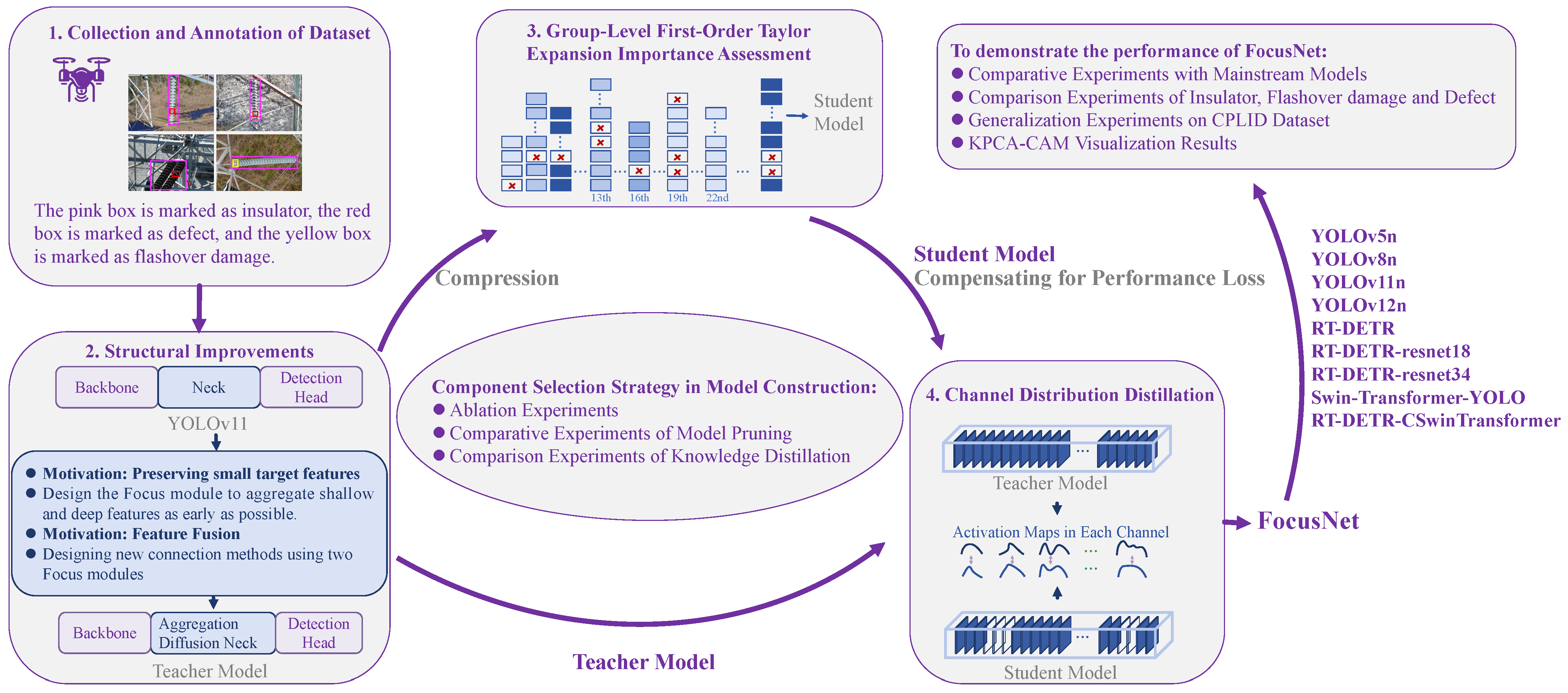
Research Roadmap. The framework follows a phased process: 1. Dataset construction (UAV image collection with DJI M300 + LabelImg annotation); 2. Teacher model development (Focus module design + Aggregation Diffusion Neck construction); 3. Model compression (Group-Level First-Order Taylor Expansion pruning to generate student model, where the red "X" symbol indicates that the channel in the convolution layer is removed during the pruning process); 4. Performance compensation (Channel Distribution Distillation strategy); 5. Scheme optimization (ablation, pruning, and distillation comparison experiments); 6. Model verification (comparative experiments with mainstream models like YOLO series and RT-DETR series).
Figure 2.
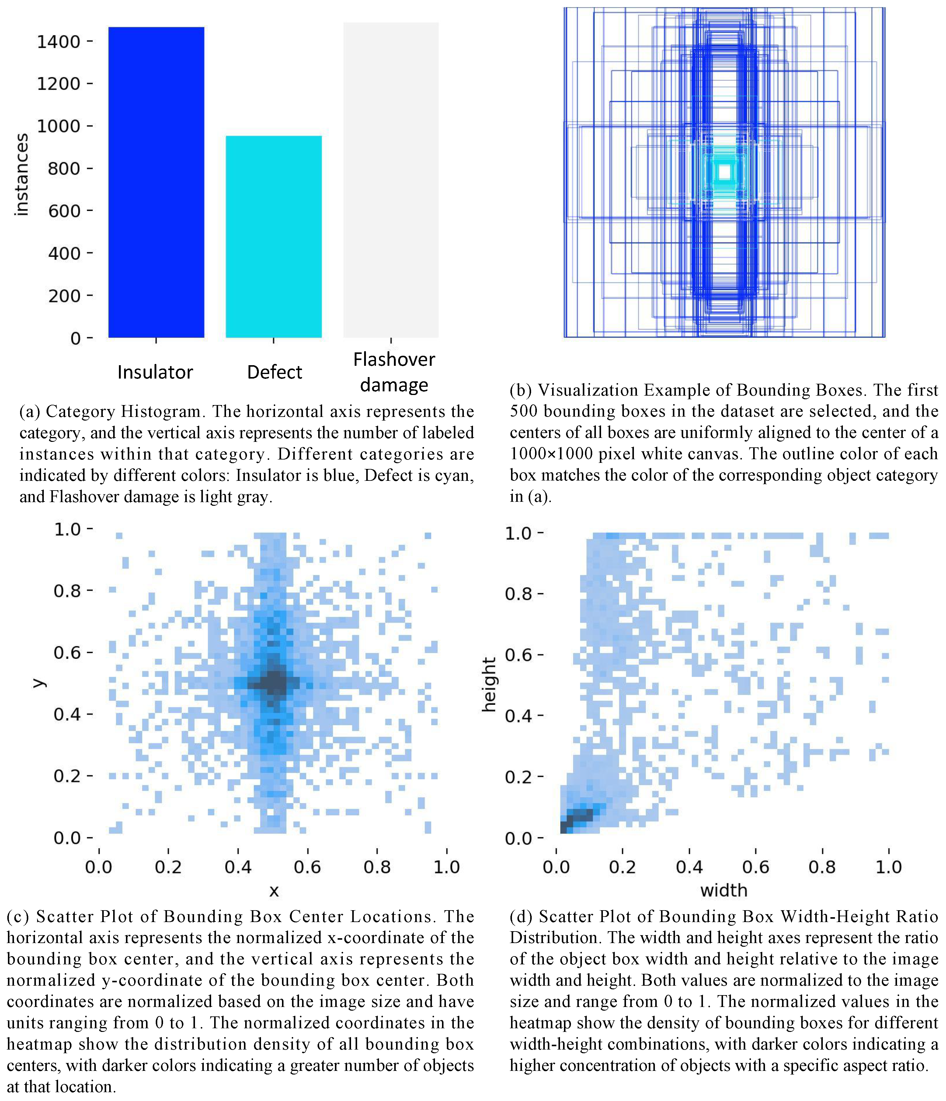
Labeling and Data Distribution. This figure presents a visual analysis of the insulator defect dataset, including the category count distribution, annotation box distribution, target centroid distribution, and width–height distribution of the detected targets.
Figure 2.
Labeling and Data Distribution. This figure presents a visual analysis of the insulator defect dataset, including the category count distribution, annotation box distribution, target centroid distribution, and width–height distribution of the detected targets.
Figure 3.
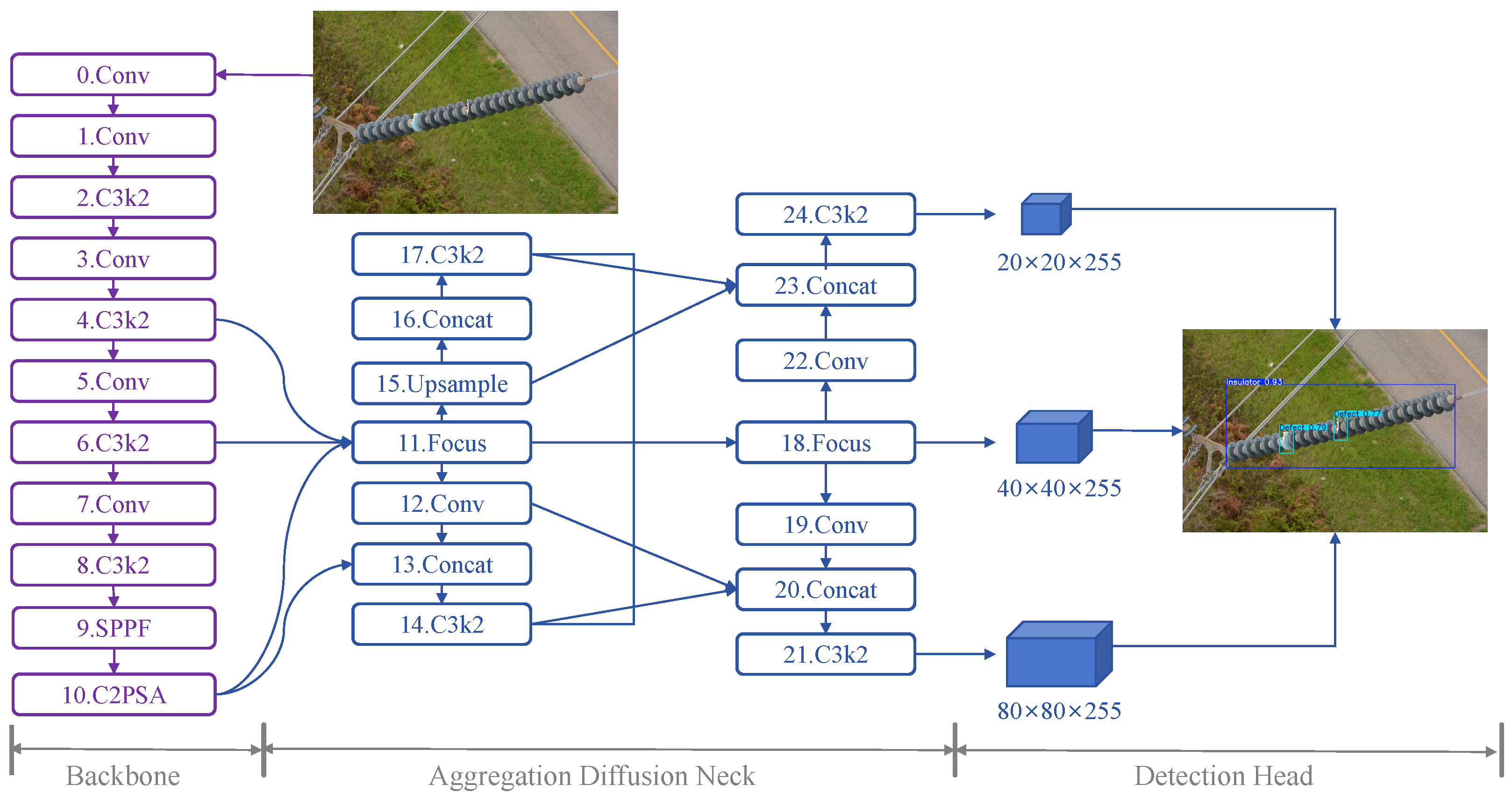
The structure of FocusNet. Aggregation Diffusion Neck is an innovation in the network structure. The Focus module and Concat aggregate feature maps with different numbers of channels and different receptive field sizes. The C3k2, Conv, and Upsample modules diverge feature maps to multiple aggregation blocks.
Figure 4.
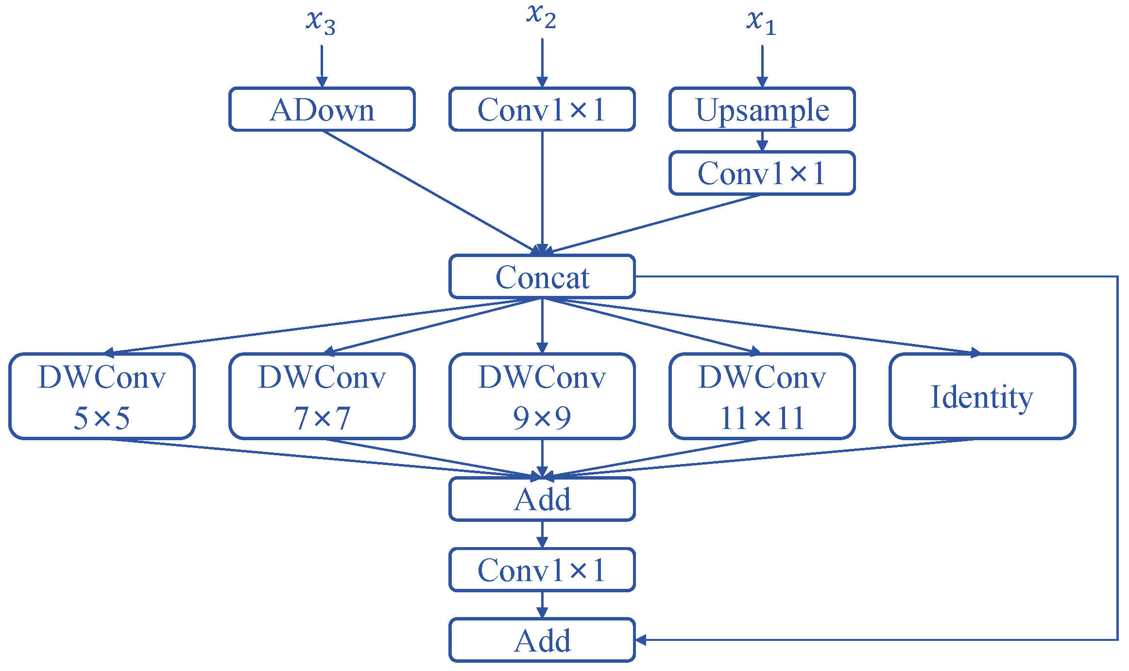
Focus. This is a neural network module structure for feature fusion and multi-scale feature extraction. ADown is adaptive downsampling, which is used to adjust the size of feature maps. convolution is used to adjust the number of channels. Upsample is used to increase the resolution so that high-level features can be aligned with low-level features in size. DWConv contains four convolution kernels of different sizes and is used to extract features with different receptive fields. Identity represents directly passing the original features to retain basic information. Add means performing element-wise addition on the output tensors of multiple branches to fuse features with different receptive fields.
Figure 5.
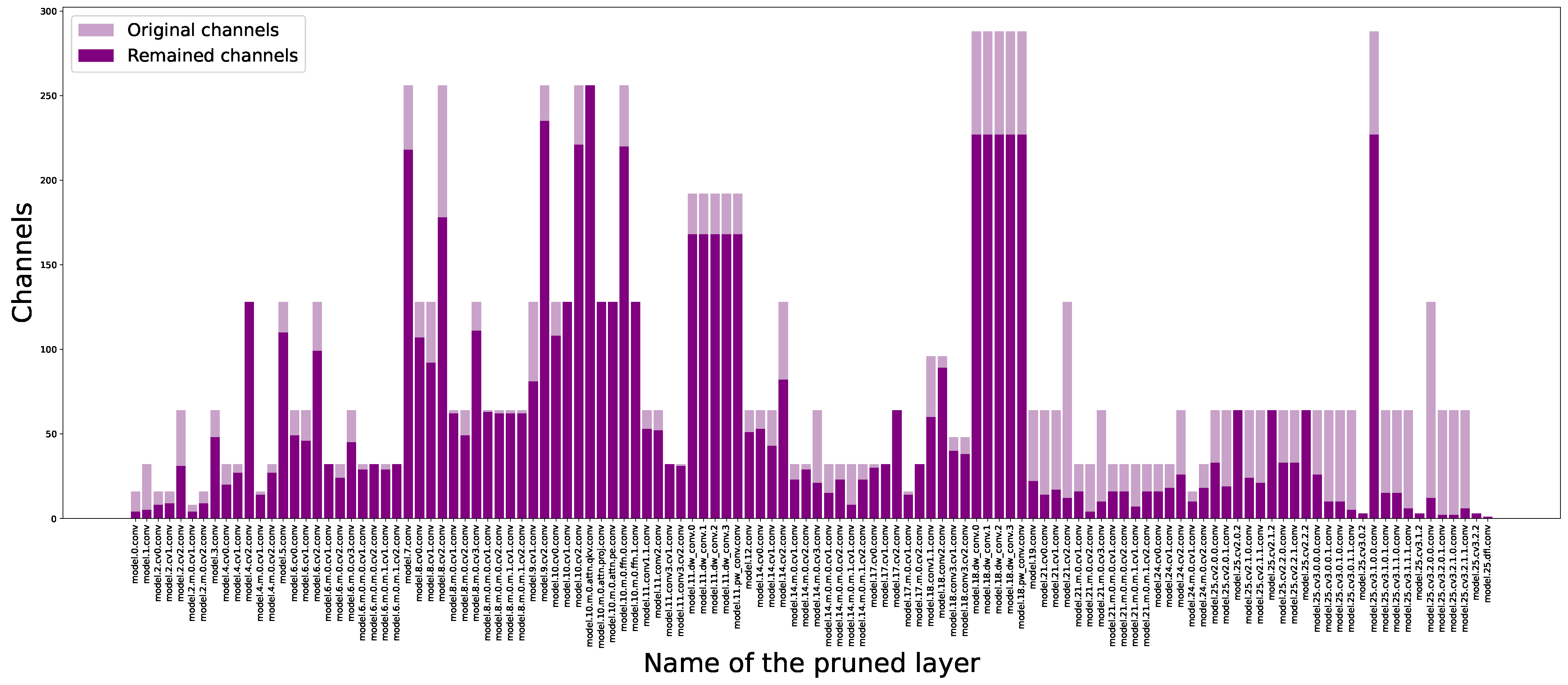
Group-Level First-Order Taylor Expansion Importance Assessment Method. The horizontal axis represents the name of the pruned layer, and the vertical axis represents the number of channels, ranging from 0 to 300. Two colors are used in the figure to distinguish data: light purple represents the number of channels in the original model, and dark purple represents the number of channels in the pruned model, visually showing the difference in the number of channels in each layer before and after pruning.
Figure 6.
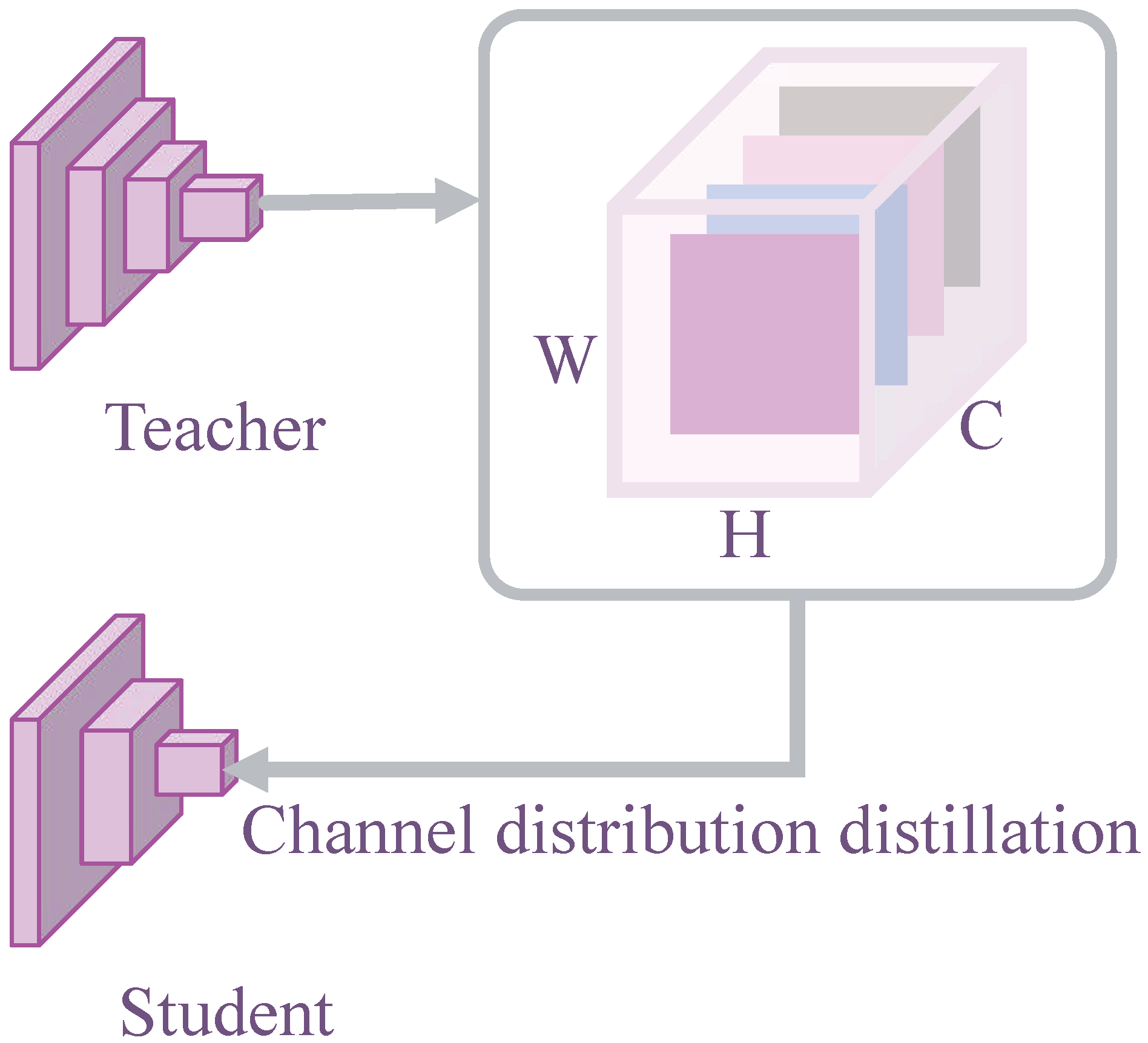
Knowledge Distillation. C represents the number of channels in the feature map, W represents the width of the feature map, and H represents the height of the feature map.
Figure 6.
Knowledge Distillation. C represents the number of channels in the feature map, W represents the width of the feature map, and H represents the height of the feature map.
Figure 7.
Verification Demonstration. These are visualizations of batch results from the validation phase of our self-built insulator dataset. The images show insulators of varying colors and structures, with the locations of the insulators and defects clearly circled in each image. Flashover damage, a frequently occurring defect, is labeled white in many images. Defects, which occur less frequently, are labeled cyan.
Figure 8.
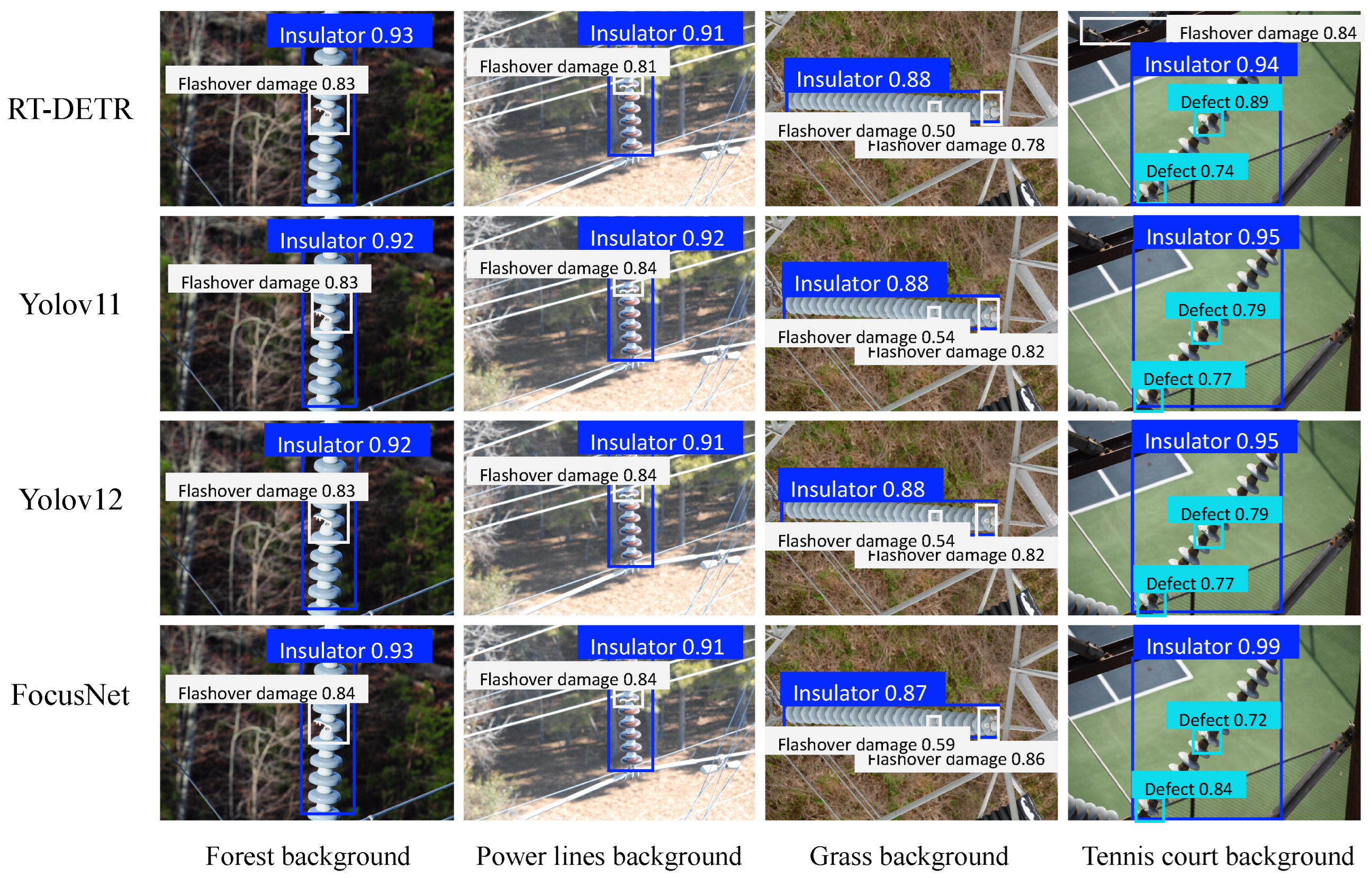
Detection Results. These are the detection results of different object detection models for insulator, flashover damage, and defect in four different backgrounds (forest, power lines, grassland, and tennis court). The results include the category names and confidence levels. Insulators are marked in blue, defects in cyan, and flashover damage in white.
Figure 9.
Precision Changes during training. This figure shows the changing trend of the precision of different improved versions of the Yolov11n model during training with the number of training epochs. At the same time, the zoomed-in figure focuses on the accuracy details in the later stages of training (Epoch 480–500).
Figure 10.
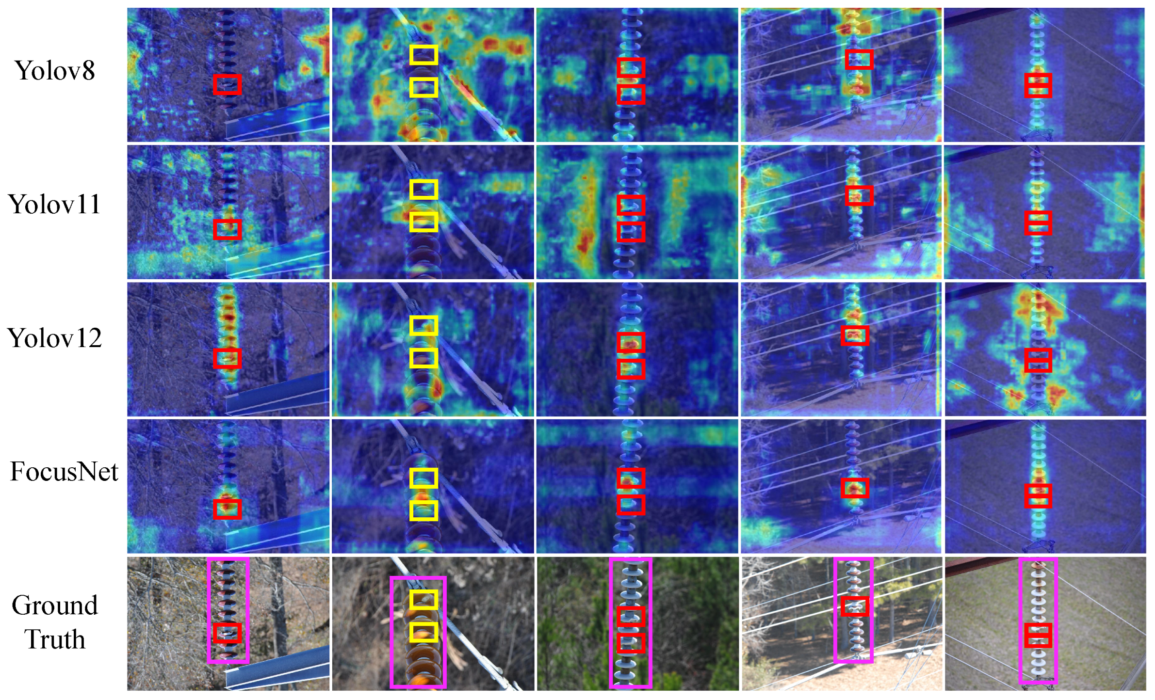
KPCA-CAM visual interpretability. The red areas in the heat map represent high-response areas that the model focuses on, and the blue areas are low-response background. The pink box is marked as insulator, the red box is marked as defect, and the yellow box is marked as flashover damage.
Figure 10.
KPCA-CAM visual interpretability. The red areas in the heat map represent high-response areas that the model focuses on, and the blue areas are low-response background. The pink box is marked as insulator, the red box is marked as defect, and the yellow box is marked as flashover damage.
Table 1.
Insulator dataset.
Table 1.
Insulator dataset.
| Category | Insulator | Defect | Flashover Damage |
|---|
| Instance number | 2183 | 1460 | 2146 |
| Image pixels | | | |
| Shooting distance | 5–7 m (consistent for all categories) |
| Shooting angle | 30°–80° (Angle from horizontal plane) |
| Shooting background | Rivers, vegetation, mountains, farmland, transmission tower, conductors |
| Weather conditions | Sunny, cloudy, overcast |
Table 2.
Hyperparameter settings for model training.
Table 2.
Hyperparameter settings for model training.
| Hyperparameters | Value | Hyperparameters | Value |
|---|
| Image size | 640 × 640 | Epoch | 500 |
| Weight decay | 0.0005 | Batch size | 32 |
| Momentum | 0.937 | Learning rate | 0.01 |
Table 3.
Comparative experiments of mainstream models. Black bold font indicates the optimal result, and ‘‘–’’ means missing data.
Table 3.
Comparative experiments of mainstream models. Black bold font indicates the optimal result, and ‘‘–’’ means missing data.
| Model | P% | R% | mAP@0.5% | mAP@0.5:0.95% | Params | GFLOPs | Memory |
|---|
| SSD | 89.28 | 73.78 | 84.11 | – | 34.31 | – | – |
| Faster R-CNN | 58.61 | 88.75 | 81.43 | – | 41.53 | – | – |
| YOLOv5n | 97.00 | 94.80 | 97.90 | 78.00 | 2.20 | 5.80 | 4.70 |
| YOLOv8n | 97.30 | 97.30 | 98.80 | 81.10 | 2.70 | 6.80 | 5.70 |
| YOLOv11n | 95.60 | 96.90 | 98.50 | 80.50 | 2.60 | 6.30 | 5.50 |
| YOLOv12n | 97.30 | 95.10 | 98.60 | 79.70 | 2.60 | 6.30 | 5.50 |
| RT-DETR | 96.70 | 95.70 | 98.90 | – | 2.50 | – | – |
| RT-DETR-resnet18 | 98.40 | 97.50 | 98.40 | 80.20 | 19.90 | 56.90 | 80.70 |
| RT-DETR-resnet34 | 97.90 | 97.90 | 98.90 | 79.00 | 31.10 | 88.80 | 125.70 |
| Swin-Transformer-YOLO | 96.90 | 96.60 | 98.30 | 78.40 | 29.70 | 77.60 | 60.00 |
| RT-DETR-CSwinTransformer | 97.20 | 98.20 | 99.20 | 80.80 | 30.50 | 89.90 | 123.20 |
| FocusNet | 98.50 | 98.50 | 99.20 | 83.50 | 1.40 | 3.80 | 3.40 |
Table 4.
Ablation experiment.
Table 4.
Ablation experiment.
| Model | R% | mAP@0.5:0.95% | Params | GFLOPs |
|---|
| YOLOv11n | 96.90 | 80.50 | 2.60 | 6.30 |
| YOLOv11n+ Aggregation Diffusion Neck | 97.80 | 82.70 | 2.70 | 7.60 |
| YOLOv11n+ Aggregation Diffusion Neck+ Group Taylor | 98.20 | 82.10 | 1.40 | 3.80 |
| YOLOv11n+ Aggregation Diffusion Neck+ Group Taylor+ CDD | 98.50 | 83.50 | 1.40 | 3.80 |
Table 5.
Comparative experiments of model pruning. Black bold font indicates the optimal result.
Table 5.
Comparative experiments of model pruning. Black bold font indicates the optimal result.
| Model | R% | mAP@0.5% | Params | Memory |
|---|
| Slim [30] | 97.60 | 99.10 | 1.40 | 3.10 |
| Group norm [31] | 96.50 | 98.30 | 2.00 | 4.40 |
| Group sl [31] | 98.10 | 98.10 | 1.50 | 3.40 |
| Group Taylor | 98.50 | 99.20 | 1.40 | 3.40 |
Table 6.
Comparative experiments on knowledge distillation. Black bold font indicates the optimal result.
Table 6.
Comparative experiments on knowledge distillation. Black bold font indicates the optimal result.
| Model | P% | R% | mAP@0.5% | mAP@0.5:0.95% |
|---|
| MIMIC [32] | 97.30 | 98.40 | 99.10 | 83.30 |
| L1 | 97.20 | 98.70 | 98.90 | 83.40 |
| L2 | 97.30 | 98.3 | 98.80 | 82.90 |
| CDD | 98.50 | 98.50 | 99.20 | 83.50 |
Table 7.
Comparison experiments of insulator, flashover damage, and defect.
Table 7.
Comparison experiments of insulator, flashover damage, and defect.
| | Model | P% | R% | mAP@0.5% | mAP@0.5:0.95% |
|---|
| Insulator | YOLOv5n | 98.60 | 99.30 | 99.20 | 94.80 |
| YOLOv8n | 98.50 | 99.70 | 99.40 | 95.70 |
| YOLOv11n | 98.30 | 99.70 | 99.50 | 96.00 |
| RT-DETR | 98.60 | 99.70 | 99.50 | 90.30 |
| RT-DETR-resnet18 | 98.60 | 100.00 | 99.50 | 89.70 |
| FocusNet | 98.90 | 100.00 | 99.50 | 96.40 |
| Flashover damage | YOLOv5n | 95.00 | 90.20 | 95.70 | 66.80 |
| YOLOv8n | 96.00 | 90.20 | 97.50 | 67.80 |
| YOLOv11n | 93.00 | 93.60 | 97.10 | 69.10 |
| RT-DETR | 95.40 | 98.80 | 98.40 | 73.40 |
| RT-DETR-resnet18 | 97.60 | 99.60 | 98.40 | 73.20 |
| FocusNet | 97.90 | 96.90 | 98.50 | 73.70 |
| Defect | YOLOv5n | 97.50 | 94.70 | 98.90 | 72.40 |
| YOLOv8n | 97.50 | 95.40 | 98.80 | 75.60 |
| YOLOv11n | 95.60 | 97.40 | 98.90 | 75.90 |
| RT-DETR | 98.50 | 98.50 | 99.50 | 77.90 |
| RT-DETR-resnet18 | 97.40 | 99.00 | 99.40 | 77.90 |
| FocusNet | 98.70 | 99.40 | 99.40 | 80.30 |
Table 8.
Generalization experiments on CPLID dataset. Black bold font indicates the optimal result, and ‘‘–’’ means missing data.
Table 8.
Generalization experiments on CPLID dataset. Black bold font indicates the optimal result, and ‘‘–’’ means missing data.
| Model | P% | R% | mAP@0.5% | Params | GFLOPs |
|---|
| Improved Faster R-CNN [19] | – | – | 92.00 | – | 24.00 |
| Improved YOLOv3 [24] | 98.00 | 95.00 | 96.50 | – | – |
| Improved YOLOv4 [25] | 93.80 | 93.99 | 97.26 | – | – |
| ID-YOLO [26] | 92.14 | – | 95.60 | 5.90 | – |
| Insu-YOLO [27] | – | – | 95.90 | – | 13.80 |
| YOLOv5n | 96.40 | 97.90 | 99.10 | 2.10 | 5.80 |
| YOLOv8n | 95.40 | 97.40 | 99.00 | 2.60 | 6.80 |
| YOLOv11n | 95.10 | 98.40 | 98.90 | 2.50 | 6.30 |
| YOLOv12n | 98.00 | 96.30 | 99.00 | 2.56 | 6.30 |
| RT-DETR | 96.40 | 98.10 | 99.20 | 32.00 | 103.4 |
| RT-DETR-resnet18 | 94.70 | 97.40 | 99.10 | 19.87 | 56.90 |
| RT-DETR-resnet34 | 96.80 | 97.20 | 99.00 | 31.11 | 88.80 |
| Swin-Transformer-YOLO | 97.20 | 98.40 | 99.10 | 29.72 | 77.60 |
| RT-DETR-CSwinTransformer | 95.90 | 97.20 | 98.90 | 30.49 | 89.90 |
| FocusNet | 98.90 | 99.20 | 99.20 | 1.40 | 3.80 |
