Analysis and Simulation of Polishing Robot Operation Trajectory Planning

Abstract

Trajectory planning is essential for robotic polishing tasks, as the effectiveness of this planning directly influences the quality of the work and the energy efficiency of the operation. This study introduces an innovative trajectory planning method for robotic polishing tasks, focusing on the development and application of quintic B-spline interpolation. Recognizing the critical impact of trajectory planning on the quality and energy efficiency of robotic operations, we analyze the structure and parameters of the ABB-IRB120 robot within a laboratory setting. Using the Denavit–Hartenberg parameter method, a kinematic model is established, and the robot’s motion equations are derived through matrix transformation. We then propose a novel approach by implementing both fifth-degree polynomial and quintic B-spline interpolation algorithms for planning the robot’s spatial spiral arc trajectory, which is a key contribution of this work. The effectiveness of these methodologies is validated through simulation in MATLAB’s robotics toolbox. Our findings demonstrate that the quintic B-spline interpolation not only significantly improves task precision but also optimizes energy consumption, making it a superior method for trajectory planning in robotic grinding applications. By integrating advanced interpolation techniques, this study provides substantial technological and environmental benefits, offering a groundbreaking reference for enhancing the precision and efficiency of robotic control systems.

1. Introduction

With the development of modern science and technology, robots are widely used in various production industries, which greatly improves the efficiency of industrial production. In the realm of manufacturing, the precision and efficiency of grinding robots are largely contingent upon the optimization of their trajectory planning. The core scientific problem addressed in this study is the optimization of trajectory planning to enhance both the precision and energy efficiency of robotic grinding operations. Trajectory planning is a pivotal aspect of robot motion control, encompassing the generation and optimization of motion paths for the robot’s end-effector (e.g., a grinding tool) to facilitate efficient and precise grinding operations. This involves addressing the scientific challenge of optimizing both the accuracy and the energy consumption of the robotic operations. The quality of trajectory planning affects the movement effect of the robot and then affects the quality of grinding. Trajectory planning is the prerequisite for achieving optimal performance in grinding robots. Linear and arc trajectory planning are two basic trajectory planning methods. Because the planned trajectory is relatively simple, the application surface is narrow. Traditional trajectory planning techniques have many drawbacks, such as not finding a global solution, requiring gradients, not being used for discontinuous functions, etc. [1]. More and more scholars adopt intelligent algorithms in path planning, such as the particle swarm optimization (PSO) [2], genetic algorithm [3,4], ant colony algorithm [5], artificial bee colony algorithm [6,7], and so on. These intelligent algorithms aim to overcome the limitations of traditional methods and address the core scientific challenge of enhancing trajectory precision while reducing energy consumption.

Fang et al. [8] use an improved B-spline interpolation method to optimize the joint trajectory of the welding robot and verify the feasibility of this method through simulation experiments. It effectively enhances the smooth continuity of the angular values and angular velocity values of each joint’s trajectory, making the robot’s operation smoother and more stable [9]. Feng [10] and Zhou [11] perform kinematic analysis on the joints of the ABB IRB140 grinding robot, establish a robot model using an enhanced DH method, and deduce both forward and inverse kinematic equations through the analysis of the robot’s geometric relationships and joint variables. Trajectory planning is carried out using the quintic polynomial function method, yielding improved joint trajectories and end-effector trajectory curves through simulation. In reference [12], Alaa Saadah et al. applied MATLAB to trajectory planning for the arc welding of a KUKA KR5 robot. The trajectory planning and simulation of the robot operation were realized utilizing the Jacobian matrix of linear paths and circular paths. The achievement of good results was tested through experimental setups. Wang Lei and others used a beetle swarm optimization algorithm for trajectory planning of robotic manipulators [3]. The beetle antennae search algorithm has distinct advantages in dealing with low-dimensional trajectory optimization problems. However, it may face efficiency issues in high-dimensional problems, such as trajectory planning for a six-axis robot, and its universality and robustness still need to be verified. Yunjeong and Byung Kook [13] propose a time-optimal trajectory planning algorithm for differential drive-wheeled mobile robots. By segmenting the trajectory and employing the bang-bang principle, it achieves rapid and safe mobility. The authors in [14,15,16] also propose a time-optimal trajectory planning algorithm for robot applications, achieving good results. Studies in the literature [6,11,17,18,19,20] made corresponding trajectory planning or optimization research for different robots, which achieved certain expected results.

Our study aims to further these efforts by addressing the dual challenges of optimizing trajectory precision and energy efficiency, particularly through the comparative study of fifth-degree polynomial and B-spline interpolation algorithms. This paper, with spiral arc trajectory as an example, through the simulation model in MATLAB R2021a/SIMULINK, aims to design the ABB-IRB120 six-axis robot model, build the robot space arc grinding trajectory motion model, take five polynomial interpolation algorithms and five B spline interpolation algorithms for comparative study, select the trajectory planning method to eliminate the grinding robot jitter in motion, and improve the quality of grinding.

To provide a clearer outline of our work, this paper is organized as follows: In Section 2, we detail the establishment of the kinematic model for the ABB-IRB120 robot and describe our approach to modeling the spatial spiral curve trajectory. In Section 3, we discuss the application of quintic polynomial and B-spline interpolation algorithms, present the simulation results assessing their effectiveness and efficiency, and rigorously validate these methods through detailed comparative analyses. Finally, in Section 4 we summarize the findings and discuss the implications of our work, highlighting potential areas for future research.

2. Materials and Methods

2.1. The Establishment of the Robotic Arm Kinematics Model and the Spatial Spiral Curve Model

2.1.1. Robot Kinematics and Modeling

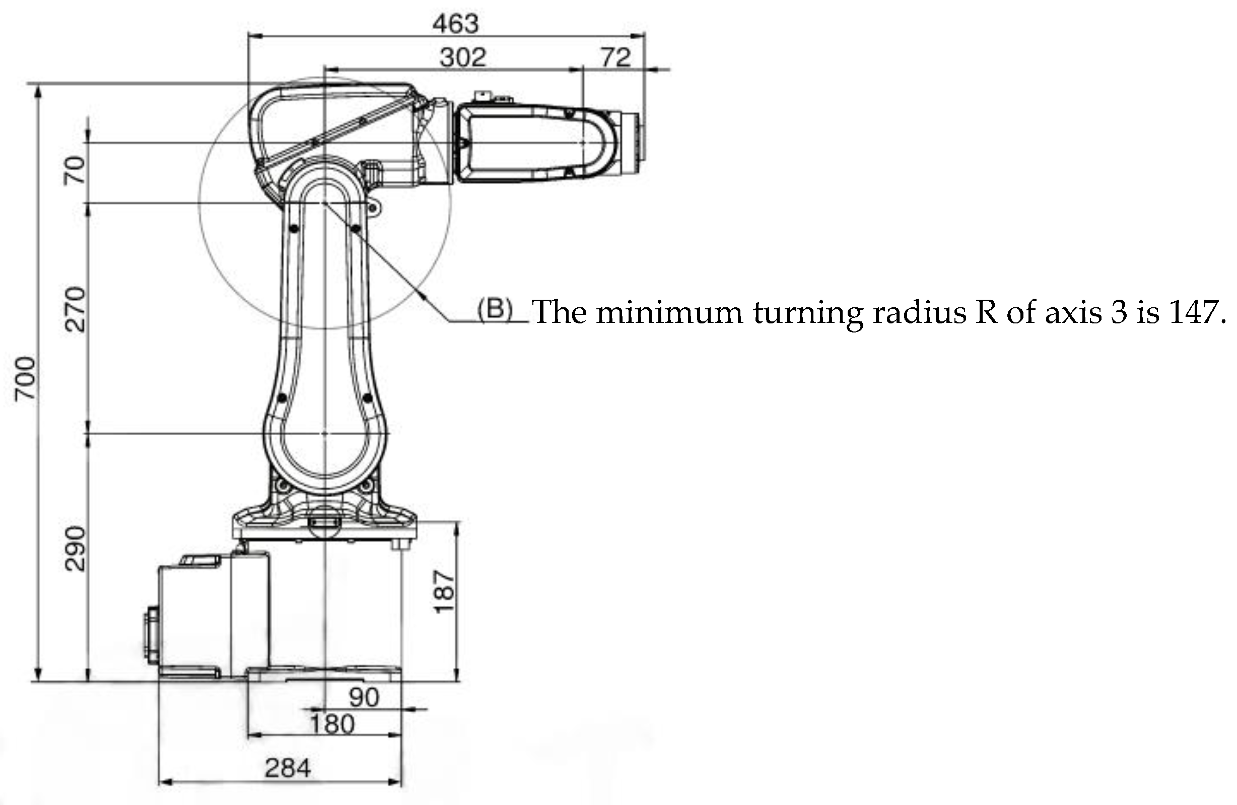
The ABB-IRB120, as a compact six-axis industrial robot, has been widely adopted in the manufacturing industry due to its high precision, exceptional flexibility, and reliability. Figure 1 illustrates the planar schematic diagram of the ABB-IRB120 six-axis robot, which provides a clear visual representation of the robot’s structural composition and relationship between its various links. This schematic serves as a foundational basis for understanding the robot’s kinematic and dynamic characteristics.

The link parameters of the ABB IRB120 robot are critical in defining its motion capabilities and performance. The link parameters for the ABB IRB120 polishing robot are referenced in the literature [8,21]. These parameters, such as link lengths, twist angles, and offset distances, are essential components of the robot’s kinematic model and are used to calculate its forward and inverse kinematics.

Table 1. The D-H parameters table for the ABB-IRB120 six-axis robot.

Link Rod i	Twist Angle ${\mathit{\alpha }}_{\mathit{i}-1}$/Rad	Link Length ${\mathit{a}}_{\mathit{i}-1}$/mm	Joint Angle ${\mathit{\theta }}_{\mathit{i}}$/rad	Link Offset ${\mathit{d}}_{\mathit{i}}$/mm	Other
1	0	0	$\theta$1	l1	1l = 290 mm
2	−π/2	0	$\theta$2−π/2	0	—
3	0	l2	$\theta$3	0	l2 = 270 mm
4	−π/2	l3	$\theta$4	l4	l3 = 70 mm l4 = 302 mm
5	π/2	0	$\theta$5 + π	0	—
6	π/2	0	$\theta$6	l5	l5 = 72 mm

presents the comprehensive DH (Denavit–Hartenberg) parameter table for the ABB-IRB120 six-axis robot. By using these parameters, it is possible to accurately determine the position and orientation of the robot’s end-effector relative to its base frame.

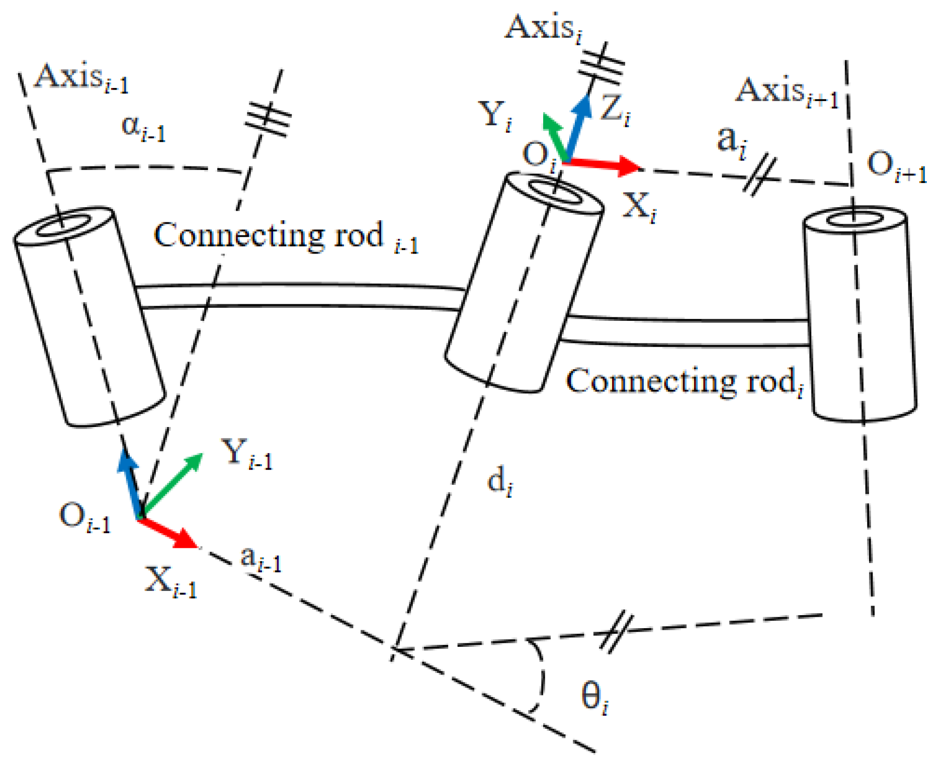
In this setup, the coordinate system for the robotic arm’s links is established using the modified DH parameters method. When studying a generalized linkage system with n joints, the homogeneous transformation matrix between adjacent links is considered, considering the neighboring links and joint Axis_i−1, Axis_i, and Axis_i+1, as shown in Figure 2.

The transformation matrix for the linkage of the improved DH coordinate system is as follows [10]:

$${{}_{}{}^{i-1}T}_i=\left|\begin{array}{cc}\begin{array}{cccc}\mathrm{c}\mathrm{o}\mathrm{s}{\theta }_i& -\mathrm{s}\mathrm{i}\mathrm{n}{\theta }_i& 0& a_{i-1}\\ \mathrm{c}\mathrm{o}\mathrm{s}{\alpha }_{i-1}\mathrm{s}\mathrm{i}\mathrm{n}{\theta }_i& \mathrm{c}\mathrm{o}\mathrm{s}{\alpha }_{i-1}\mathrm{c}\mathrm{o}\mathrm{s}{\theta }_i& -\mathrm{s}\mathrm{i}\mathrm{n}{\alpha }_{i-1}& -d_i\mathrm{s}\mathrm{i}\mathrm{n}{\alpha }_{i-1}\\ \mathrm{s}\mathrm{i}\mathrm{n}{\alpha }_{i-1}\mathrm{s}\mathrm{i}\mathrm{n}{\theta }_i& \mathrm{s}\mathrm{i}\mathrm{n}{\alpha }_{i-1}\mathrm{c}\mathrm{o}\mathrm{s}{\theta }_i& \mathrm{c}\mathrm{o}\mathrm{s}{\alpha }_{i-1}& d_i\mathrm{c}\mathrm{o}\mathrm{s}{\alpha }_{i-1}\\ 0& 0& 0& 1\end{array}& \\ & \end{array}\right|$$

(1)

where ${\alpha }_i$, $a_i$, and ${\theta }_i$ are the linkage parameters. Then, the positive kinematic equation of the robot is obtained from the pose transformation matrix of each joint of the robot [22]:

$$\begin{array}{cc}{}^{0}T_6& ={}^{0}T_1({\theta }_1)\cdot {}^{1}T_2({\theta }_2)\cdot {}^{2}T_3({\theta }_3)\cdot {}^{3}T_4({\theta }_4)\cdot {}^{4}T_5({\theta }_5)\cdot {}^{5}T_6({\theta }_6)\\ & =\left[\begin{array}{cc}\begin{array}{cccc}{n}_x& o_x& a_x& p_x\\ n_y& o_y& a_y& p_y\\ n_z& o_z& a_z& p_z\\ 0& 0& 0& 1\end{array}& \\ & \end{array}\right]\end{array}$$

(2)

Here,

$$\begin{gathered} n_x=s{\theta }_6\left[c{\theta }_{1}s{\theta }_{4}s({\theta }_2+{\theta }_3)-c{\theta }_{4}s{\theta }_1\right]-c{\theta }_6\left[c{\theta }_{5}s{\theta }_{1}s{\theta }_4+c{\theta }_{1}s{\theta }_{5}c({\theta }_2+{\theta }_3)+c{\theta }_{1}c{\theta }_{4}c{\theta }_{5}s({\theta }_2+{\theta }_3)\right] \\ {n}_y=s{\theta }_6\left[c{\theta }_{1}c{\theta }_4+s{\theta }_{1}s{\theta }_{4}s({\theta }_2+{\theta }_3)\right]-c{\theta }_6\left[s{\theta }_{1}s{\theta }_{5}c({\theta }_2+{\theta }_3)-c{\theta }_{1}c{\theta }_{5}s{\theta }_4+c{\theta }_{4}c{\theta }_{5}s{\theta }_{1}s({\theta }_2+{\theta }_3)\right] \\ {n}_z=c{\theta }_6\left[s{\theta }_{5}s({\theta }_2+{\theta }_3)-c{\theta }_{4}c{\theta }_{5}c({\theta }_2+{\theta }_3)\right]+s{\theta }_{4}s{\theta }_{6}c({\theta }_2+{\theta }_3) \\ {o}_x=c{\theta }_6\left[c{\theta }_{1}s{\theta }_{4}s({\theta }_2+{\theta }_3)-c{\theta }_{4}s{\theta }_1\right]+s{\theta }_6\left[c{\theta }_{5}s{\theta }_{1}s{\theta }_4+c{\theta }_{1}s{\theta }_{5}c({\theta }_2+{\theta }_3)+c{\theta }_{1}c{\theta }_{4}c{\theta }_{5}s({\theta }_2+{\theta }_3)\right] \\ {o}_y=c{\theta }_6\left[c{\theta }_{1}c{\theta }_4+s{\theta }_{1}s{\theta }_{4}s({\theta }_2+{\theta }_3)\right]+c{\theta }_6\left[s{\theta }_{1}s{\theta }_{5}c({\theta }_2+{\theta }_3)-c{\theta }_{1}c{\theta }_{5}s{\theta }_4+c{\theta }_{4}c{\theta }_{5}s{\theta }_{1}s({\theta }_2+{\theta }_3)\right] \\ {o}_z=c{\theta }_{6}s{\theta }_{4}c({\theta }_2+{\theta }_3)-s{\theta }_6\left[s{\theta }_{5}s({\theta }_2+{\theta }_3)-c{\theta }_{4}c{\theta }_{5}c({\theta }_2+{\theta }_3)\right] \\ {p}_x=c{\theta }_1\left[ls{\theta }_2+c{\theta }_{1}c{\theta }_{4}s({\theta }_2+{\theta }_3)\right] \\ {p}_y=c{\theta }_{1}c{\theta }_{5}c({\theta }_2+{\theta }_3)-s{\theta }_5\left[c{\theta }_{4}s{\theta }_{1}s({\theta }_2+{\theta }_3)-c{\theta }_{1}c{\theta }_4\right] \\ {p}_z=-c{\theta }_{5}s({\theta }_2+{\theta }_3)-c{\theta }_{4}s{\theta }_{5}c({\theta }_2+{\theta }_3) \\ {p}_x=c{\theta }_1\left[l_{2}s{\theta }_2+l_{3}s({\theta }_2+{\theta }_3)+l_{4}c({\theta }_2+{\theta }_3)+l_{5}c{\theta }_{5}c({\theta }_2+{\theta }_3)-l_{5}c{\theta }_{4}s{\theta }_{5}s({\theta }_2+{\theta }_3)\right]-l_{5}s{\theta }_{1}s{\theta }_{4}s{\theta }_5 \\ {p}_y=s{\theta }_1\left[l_{2}s{\theta }_2+l_{3}s({\theta }_2+{\theta }_3)+l_{4}c({\theta }_2+{\theta }_3)+l_{5}c{\theta }_{5}c({\theta }_2+{\theta }_3)-l_{5}c{\theta }_{4}s{\theta }_{5}s({\theta }_2+{\theta }_3)\right]+l_{5}c{\theta }_{1}s{\theta }_{4}s{\theta }_5 \\ {p}_z=l_1+l_{2}c{\theta }_2+l_{3}c({\theta }_2+{\theta }_3)-l_{4}s({\theta }_2+{\theta }_3)-l_{5}c{\theta }_{5}s({\theta }_2+{\theta }_3)-l_{5}c{\theta }_{4}s{\theta }_{5}s({\theta }_2+{\theta }_3) \end{gathered}$$

In the formulas, cθ = cosθ, sθ = sinθ, [n_x, n_y, n_z]^T, [o_x, o_y, o_z]^T, [a_x, a_y, a_z]^T, [p_x, p_y, p_z]^T represent, respectively, the normal vector, orientation vector, approach vector of the end-effector in the base coordinate system, and the position vector of the end-effector in the base coordinate system [10]. After obtaining the above terminal pose matrix of the robot, we analyze the inverse kinematics of the robot and solve the motion variables of each joint of the robot, and the solution of θ is obtained by the inverse kinematics as follows:

The first joint variable θ₁ can be obtained as follows:

θ₁:θ₁ = atan2(p_y− l₅a_y, p_x − l₅a_x)

(3)

The 2nd joint variable θ₂ can be obtained as follows:

$${\theta }_2=a\mathit{tan}2(A_2,\pm \sqrt{1-A_2^2})-{\varphi }_2$$

(4)

In this formula,

$$A_2={\displaystyle \frac{l_2^2-l_3^2-l_4^2+{\left[c{\theta }_1(p_x-l_5{a}_x)+s{\theta }_1(p_y-l_5{a}_y)\right]}^2+(p_z-l_1-l_5{a}_z{)}^2}{2l_2}},$$

$${\varphi }_2=a\mathit{tan}2(p_z-l_1-l_5{a}_z,c{\theta }_1(p_x-l_5{a}_x)+s{\theta }_1(p_y-l_5{a}_y))$$

The third joint variable θ₃ can be obtained as follows:

$${\theta }_3=a\mathit{tan}2(c{\theta }_1(p_x-l_5{a}_x)+s{\theta }_1(p_y-l_5{a}_y)-l_{2}s{\theta }_2,p_z-l_1-l_5{a}_z-l_{2}c{\theta }_2)-{\theta }_2-{\varphi }_3$$

in which

$${\varphi }_3=a\mathit{tan}2(l_4,l_3)$$

(5)

The fifth joint variable θ₅ can be obtained as follows:

$${\theta }_5=a\mathit{tan}2(\pm \sqrt{1-A_5^2},A_5)$$

(6)

In this formula,

$$A_5=(a_{x}c{\theta }_1+a_{y}s{\theta }_1)c({\theta }_2+{\theta }_3)-a_{z}s({\theta }_2+{\theta }_3)$$

The fourth joint variable θ₄ can be obtained as follows:

$${\theta }_4=a\mathit{tan}2(A_{42},A_{41})$$

(7)

In this formula,

$$A_{41}={\displaystyle \frac{-(a_{x}c{\theta }_1+a_{y}s{\theta }_1)s({\theta }_2+{\theta }_3)-a_{z}c({\theta }_2+{\theta }_3)}{s{\theta }_5}},$$

$$A_{42}={\displaystyle \frac{a_{y}c{\theta }_1-a_{x}s{\theta }_1}{s{\theta }_5}}$$

The sixth joint variable θ₆ can be obtained as follows:

$${\theta }_6=a\mathit{tan}2(A_{62},A_{61})$$

(8)

In this formula,

$$A_{61}={\displaystyle \frac{-(n_{x}c{\theta }_1+n_{y}s{\theta }_1)c({\theta }_2+{\theta }_3)+n_{z}s({\theta }_2+{\theta }_3)}{s{\theta }_5}},$$

$$A_{62}={\displaystyle \frac{(o_{x}c{\theta }_1+o_{y}s{\theta }_1)c({\theta }_2+{\theta }_3)-o_{z}s({\theta }_2+{\theta }_3)}{s{\theta }_5}}$$

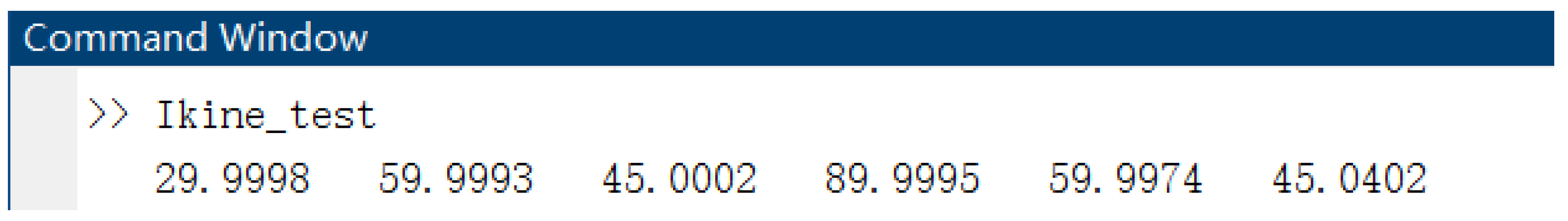
Taking the motion variables $q=({\displaystyle \frac{\pi }{6}},{\displaystyle \frac{\pi }{3}},{\displaystyle \frac{\pi }{4}},{\displaystyle \frac{\pi }{2}},{\displaystyle \frac{\pi }{3}},{\displaystyle \frac{\pi }{4}})$ as examples, the pose matrix of the end-effector can be obtained from Equation (2) as follows:

$${}^{0}T_6=\left[\begin{array}{cc}\begin{array}{cccc}0.5520& 0.6310& -0.5451& 154.1186\\ 0.7269& -0.0439& 0.6853& 160.9804\\ 0.4085& -0.7745& 0.4830& 80.3997\\ 0& 0& 0& 1.0000\end{array}& \\ & \end{array}\right]$$

(9)

Using the end pose result of Equation (9), the q = abb120_ikine(T) result is solved by the inverse kinematics equation as shown in Figure 3:

By comparing the above selection of kinematic variables $q=({\displaystyle \frac{\pi }{6}},{\displaystyle \frac{\pi }{3}},{\displaystyle \frac{\pi }{4}},{\displaystyle \frac{\pi }{2}},{\displaystyle \frac{\pi }{3}},{\displaystyle \frac{\pi }{4}})$ in forward kinematics, the results of inverse kinematics are not significantly different from the selection in forward kinematics, indicating the correctness of the established kinematics equations.

The robot multi-axis linkage angle value can be obtained through the above formula. The multi-axis linkage angle values are shown in

Table 2. Multi-axis linkage angle values.

θ1	θ2	θ3	θ4	θ5	θ6
52.7652	21.8561	18.1634	−116.0455	62.3940	−10.7425
60.7978	29.3186	6.4654	−106.6156	65.5352	−18.9757
84.7266	6.5544	34.0268	−93.3423	85.9207	−22.0362
59.7385	−9.7148	49.1090	−112.4336	68.9605	−15.9549
52.7652	19.2235	15.5904	−113.4557	60.2128	−16.1320

.

Utilizing the robotics toolbox, a three-dimensional simulation model of the ABB-IRB120 robot is constructed in MATLAB, and the simulation robot workspace is created by the Monte Carlo method. The simulation model of the robot workspace and grinding curve is shown in Figure 4. This integrated visualization offers an intuitive understanding of the robot trajectory planning.

2.1.2. Space Spiral Arc Curve Model

Suppose the radius of the spatial spiral circular arc curve is r = 100 mm, the pitch is p = 60 mm, and the inclination angle is φ₀.

Assuming that the z-axis of the spatial coordinate system w for the space spiral line to be polished coincides with the axis of the helix [9], and the spatial coordinate origin is (x_t,y_t,z_t) = (0,0,0), the parametric equations of the spiral in three-dimensional space are as follows:

$$\left\{\begin{array}{l}x=x_t+r\ast \mathit{cos}({\displaystyle \frac{2\pi }{p}}\ast \varphi )\\ y=y_t+r\ast \mathit{sin}({\displaystyle \frac{2\pi }{p}}\ast \varphi )\\ \mathrm{z}=z_t+\varphi \end{array}\right.$$

(10)

Spiral inclination angle ${\phi }_0=a\mathit{tan}2({\displaystyle \frac{p}{2\pi \ast r}})$, where φ is the variable parameter in Formula (10), φ increases from 0 equal step distance to 2p, and the parameter Equation (10) can generate the spatial spiral arc curve of the corresponding pitch p.

Suppose that the spatial coordinate system w of the spatial helix to be polished is relative to the base coordinate frame o:

$${}_w{}^{o}T=\left[\begin{array}{l}1 0 0 200\\ 0 1 0 300\\ 0 0 1 400\\ 0 0 0 1\end{array}\right]$$

(11)

In the spiral parameter equation given in Equation (10), the parametric variable φ is assigned every p/n, starting from 0 and ending when the final value is 2p. Then, obtain the junction position coordinates on the spatial spiral curves of the two pitches (x_w(i), y_w(i), z_w(i)). The total number is 2n + 1, and we can obtain the following position matrix for the 2n + 1 nodes:

$$T_w(\text{:},\text{:},i)=\left[\begin{array}{l}1 0 0 x_{w(i)}\\ 0 1 0 {\mathrm{y}}_{w(i)}\\ 0 0 1 z_{w(i)}\\ 0 0 0 1\end{array}\right]$$

(12)

Given ${}_w{}^{o}T$ and $T_w(:,:,i)$, the position matrix of selected nodes on the spatial helix in the actual workpiece coordinate system can be obtained from the formula ${}_w{}^{o}T$ and $T_w(:,:,i)$.

$$T_o(\text{:},\text{:},i)=\left[\begin{array}{l}1 0 0 x_{o(i)}\\ 0 1 0 {\mathrm{y}}_{o(i)}\\ 0 0 1 z_{o(i)}\\ 0 0 0 1\end{array}\right]$$

(13)

Through Formula (13), obtain the position of each node, connect the end position, and form the model of the spatial helical curve.

Then, solve the joint trajectory q (position), $\dot{q}$ (velocity), and $\ddot{q}$ (acceleration) of the robot when passing through each node of the spatial solid curve.

In this paper, we solve the problem of mapping the velocity of a robot in Cartesian space to the velocity in joint space using the vector product method. The displacements of the robot in Cartesian space x and joint space q can be represented by the following equations:

$$x=x(q)$$

(14)

After taking the derivative of both sides of Equation (14) concerning time, the relationship between the velocity of the robot in Cartesian space x and the velocity in joint space q is obtained as follows:

$$\stackrel{•}{x}=J(q)\stackrel{•}{q}$$

(15)

In the above formula,

$\dot{x}$ represents the velocity of the robot’s end-effector in Cartesian space;

$\dot{q}$ is the joint velocity of the robot in the joint space;

J(q) represents the Jacobian matrix for robots.

Multiplying the left-hand side of both sides of Equation (15) by J(q)⁻¹, we can obtain the formula for solving the joint speeds of the robot as follows:

$$\stackrel{•}{q}=J(q{)}^{-1}\stackrel{•}{x}$$

(16)

The velocity of the robot’s end-effector in Cartesian space is a 6-dimensional column vector, which is $\stackrel{•}{x}={\left[v_x,v_y,v_z,w_x,w_y,w_z\right]}^T$. Assuming that the velocity of the robot’s end-effector in the z-axis direction is uniform and the velocity value is v_z = 2 mm/s, the remaining velocity components of the i-th node can be expressed as

$$\left\{\begin{array}{l}{v}_x(i)=w_z(i)\ast r\ast \mathit{sin}((i-1)\ast {\alpha }_c)\\ v_y(i)=w_z(i)\ast r\ast \mathit{cos}((i-1)\ast {\alpha }_c))\\ w_x(i)=0\\ w_y(i)=0\\ w_z(i)=(2\ast \pi )/({\displaystyle \frac{p}{v_z}})\end{array}\right.$$

(17)

Here, α_c represents the step angle.

Thus, the operational speed of the robot, x, has been determined. Furthermore, from Equation (16), we can obtain the joint speed.

By taking the derivative of both sides of Equation (15), we can obtain the robot joint acceleration equation:

$$\stackrel{••}{x}=J(q)\stackrel{••}{q}+\stackrel{•}{J(q)}\stackrel{•}{q}$$

(18)

The following equation can be obtained from (18):

$$\stackrel{••}{q}=J(q{)}^{-1}[\stackrel{••}{x}-\stackrel{•}{J(q)}\stackrel{•}{q}]$$

(19)

Because the above assumes that the end speed of the robot is uniform in Cartesian space, it can be obtained as follows:

$$\stackrel{••}{x}={\left[\mathrm{0,0},\mathrm{0,0},\mathrm{0,0}\right]}^T$$

(20)

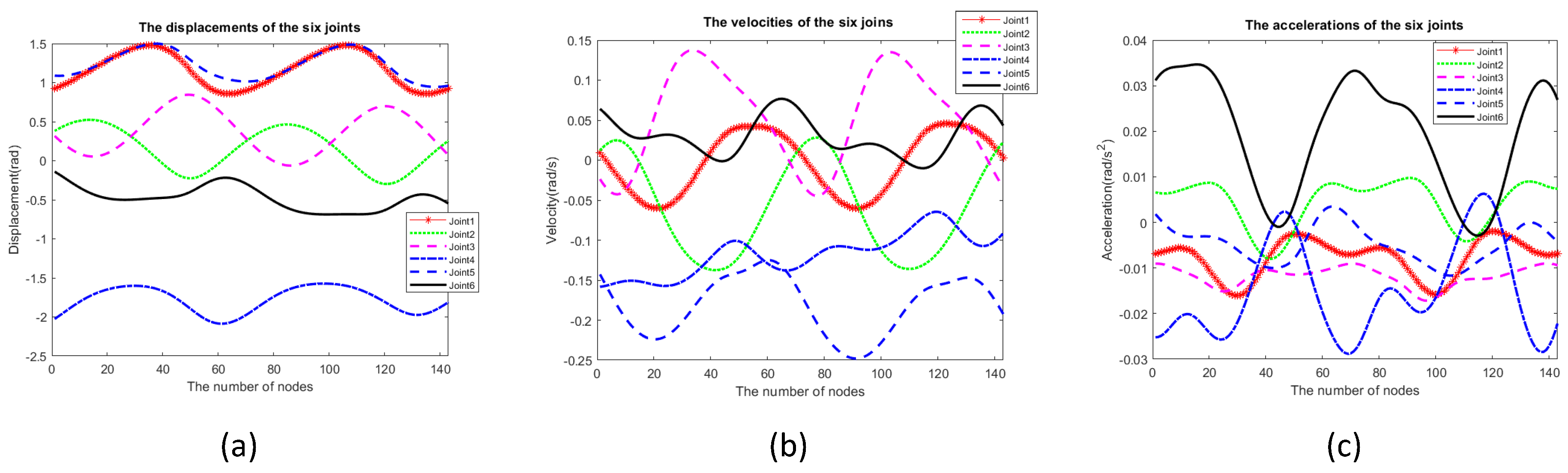
By combining Equations (18)–(20), we can solve for $\ddot{q}$. Through the calculations above and by using MATLAB for programming, we can obtain the waveforms of displacement, velocity, and acceleration for each joint, as shown in Figure 5.

2.2. Spiral Arc Trajectory Planning of Quintic Polynomial Interpolation Algorithm

Polynomial interpolation algorithms are frequently applied in trajectory planning, especially in robotics and other fields requiring smooth and precise path control. As the degree of the polynomial increases, the interpolation curve can approximate given data points more accurately, but this also introduces higher computational complexity and potential numerical instability. The quintic polynomial interpolation algorithm is a commonly used method in robot trajectory planning, as it can maintain trajectory smoothness and accuracy while relatively balancing computational complexity. It is particularly suited for planning robotic joint trajectories with continuous position, velocity, acceleration, and jerk (rate of change in acceleration), ensuring a smoother and more controlled movement. This complex algorithm utilizes the ability of polynomial functions to effectively model the complex relationship between joint displacement and time. By uniquely determining the coefficients of the polynomial based on specified boundary conditions, including the initial and final positions, velocities, and accelerations of the joint, corresponding trajectory plans can be tailored to the specific requirements of the robot and its tasks.

In the context of the quintic polynomial approach, the relationship between the joint displacement (which represents the change in position or angle of a particular joint over time) and time is expressed mathematically through a polynomial equation of the fifth degree. This equation encapsulates not just the instantaneous position of the joint at any given time but also its rate of change (i.e., velocity) and acceleration, which is beneficial to understanding the movement of the joint in its entire trajectory.

In the five-degree polynomial algorithm, the relationship between joint displacement and time is as follows:

$$\theta (t)=a_0+a_{1}t+a_2{t}^2+a_3{t}^3+a_4{t}^4+a_5{t}^5$$

(21)

For the motion trajectory of this design, for each node, only the first node, namely the time t₀ of the starting point, is zero, and the time t₀ of the other nodes is not zero. Therefore, the following equation can be obtained:

$$\left\{\begin{array}{l}\theta (0)={\theta }_0=a_0+a_1{t}_0+a_2{t}_0^2+a_3{t}_0^3+a_4{t}_0^4+a_5{t}_0^5\\ \theta (f)={\theta }_f=a_0+a_1{t}_f+a_2{t}_f^2+a_3{t}_f^3+a_4{t}_f^4+a_5{t}_f^5\\ \stackrel{•}{\theta }(0)=\stackrel{•}{{\theta }_0}=a_1+2a_2{t}_0+3a_3{t}_0^2+4a_4{t}_0^3+5a_5{t}_0^4\\ \stackrel{•}{\theta }(f)=\stackrel{•}{{\theta }_f}=a_1+2a_2{t}_f+3a_3{t}_f^2+4a_4{t}_f^3+5a_5{t}_f^4\\ \stackrel{••}{\theta }(0)=\stackrel{••}{{\theta }_0}=2a_2+6a_3{t}_0+12a_4{t}_0^2+20a_5{t}_0^3\\ \stackrel{••}{\theta }(f)=\stackrel{••}{{\theta }_f}=2a_2+6a_3{t}_f+12a_4{t}_f^2+20a_5{t}_f^3\end{array}\right.$$

(22)

In the equations, $\theta \left(0\right),\stackrel{•}{\theta }\left(0\right),\stackrel{••}{\theta }\left(0\right)\mathrm{a}\mathrm{n}\mathrm{d}\theta (f),\stackrel{•}{\theta }(f),\stackrel{••}{\theta }(f)$, respectively, represent the joint angle, angular velocity, and angular acceleration at the starting moment and ending moment. By computational solving, the values of polynomial coefficients a₀, a₁, a₂, a₃, a₄, and a₅ can be obtained.

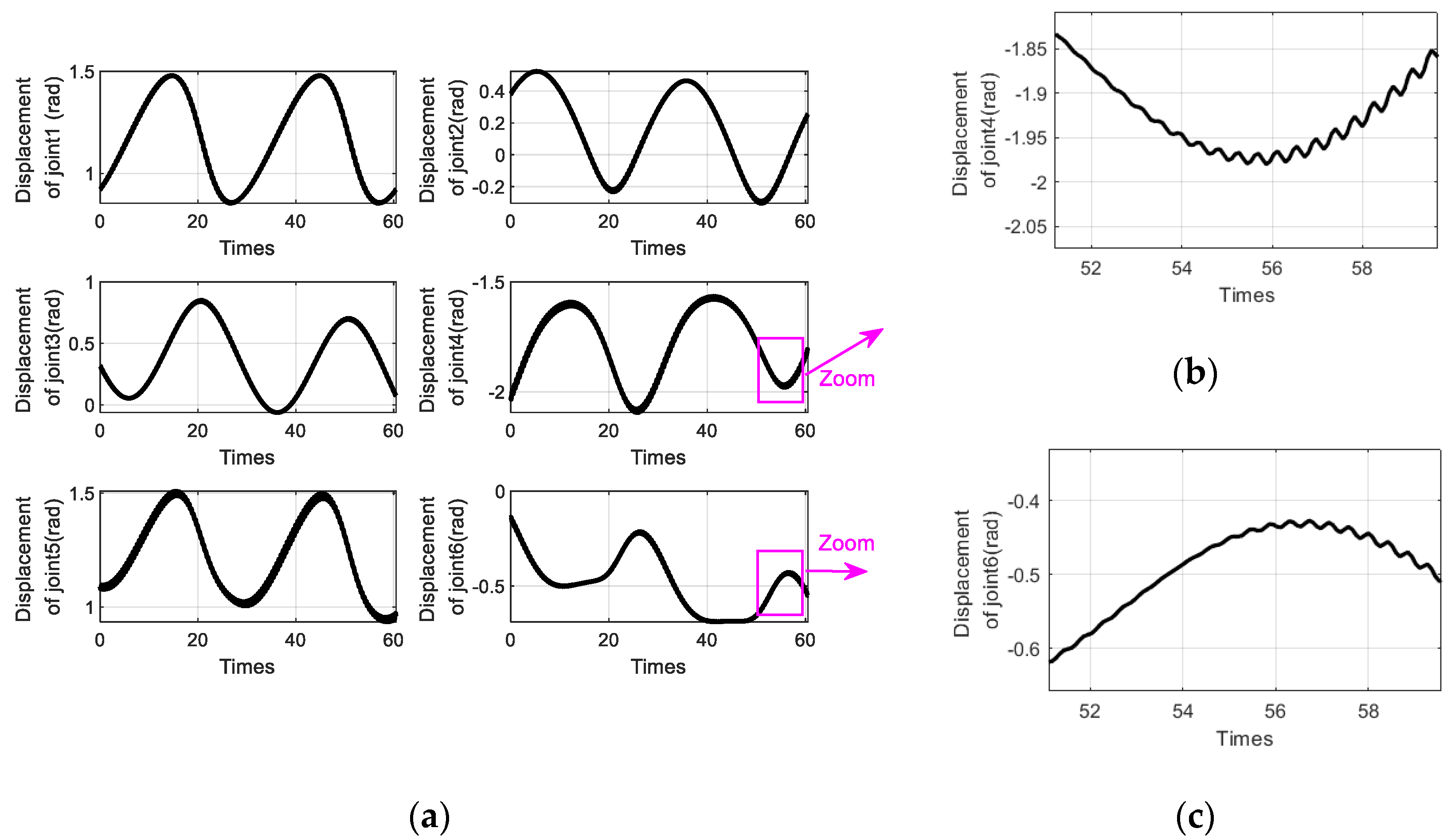
Figure 6 shows the trajectory plots for each joint of the robot, achieved using the quintic polynomial interpolation algorithm.

Figure 6 presents a visualization of the motion trajectories executed by the various joints of a robotic system, employing the quintic polynomial interpolation algorithm as its methodology. This algorithm is renowned for its ability to generate smooth and continuous motion profiles, making it a popular choice in robotics applications.

Subfigure (a) of Figure 6 specifically showcases the displacement plots for all six joints of the robot over the course of its programmed movement. These plots offer a clear overview of how each joint contributes to the overall motion of the robot, revealing the interplay between them as they work in harmony to achieve the desired task.

To gain a deeper insight into the fine-grained behavior of specific joints, subfigures (b) and (c) zoom in on certain segments of the displacement curves for joint 4 and joint 6, respectively. While the quintic polynomial interpolation algorithm is designed to ensure a smooth and seamless trajectory, upon closer inspection, one can observe minute fluctuations in the form of a sawtooth pattern within these magnified segments.

These subtle fluctuations, though seemingly insignificant, can have a non-negligible impact on the robot’s motion stability and precision. In precision-critical applications, such as assembly lines, surgical robots, or any scenario where even the slightest deviation from the intended path can lead to errors or damage, these fluctuations become a matter of concern.

Therefore, it is of great importance for us to study and formulate strategies to mitigate or eliminate these sawtooth patterns. Potential solutions may include refining the boundary conditions used in quintic polynomial interpolation, implementing additional smoothing algorithms, or exploring alternative trajectory planning methods that are inherently more stable and accurate. By solving these minor fluctuations, the overall performance and reliability of the robotic system can be significantly improved.

2.3. The Trajectory Planning of the Spiral Arc Curve Based on the Quintic B-Spline Interpolation Algorithm

The quintic B-spline interpolation algorithm is an advanced and versatile technique for crafting precise polynomial curves in numerous applications, particularly in the realm of robotics and computer-aided design. This sophisticated method employs a quintic polynomial to meticulously interpolate through a predefined set of control points, allowing for the creation of smooth and continuous trajectories.

One of the most noteworthy characteristics of the quintic B-spline interpolation is its ability to ensure continuity up to the fifth-order derivatives of the generated curve. This feature is crucial in achieving ultra-smooth transitions between segments, eliminating abrupt changes or jerks that could otherwise compromise the precision and efficiency of the system. The continuity of these higher-order derivatives also ensures that the overall shape of the curve remains predictable and manageable, facilitating the precise control of the trajectory.

Furthermore, the quintic B-spline algorithm boasts a remarkable property known as local control. This means that adjustments made to individual control points directly affect only the local segment of the curve around that point, without disturbing the global shape significantly. This localized influence is invaluable in robot path planning, where even minor modifications to the trajectory can have significant implications on the robot’s movement and performance. By enabling fine-tuned adjustments without compromising the integrity of the overall path, the quintic B-spline interpolation algorithm offers a high degree of flexibility and adaptability in designing efficient and optimal robot paths.

As we know, the quintic B-spline interpolation algorithm is a powerful tool that leverages the properties of a fifth-degree polynomial to construct smooth, continuous curves with controlled higher-order derivatives. Its local control feature further enhances its suitability for complex applications such as robot path planning, enabling precise and efficient trajectory planning in dynamic environments.

In addition to its local control and continuity properties, the quintic B-spline also falls into a broader category of B-spline curves characterized by their order. The k-th B-spline has the characteristics of order k−1, and the quintic B-spline curve has the characteristics of fourth order. The k-th B-spline curve can be represented by segmented polynomials:

$$P(t)=\sum _{i=0}^n{P}_i{F}_{i,k}(t) t\in \left[t_{k-1},t_{n+1}\right]$$

(23)

In the above equation,

$$\left\{\begin{array}{l}{F}_{i,0}(t)=\left\{\begin{array}{l}1 t_i\le t\le t_{i+1}\\ 0 \mathrm{o}\mathrm{t}\mathrm{h}\mathrm{e}\mathrm{r}\mathrm{s}\end{array}\right.\\ F_{i,k}(t)={\displaystyle \frac{t-t_i}{t_{i+k}-t_i}}{F}_{i,k-1}(t)+{\displaystyle \frac{t_{i+k+1}-t}{t_{i+k+1}-t_{i+1}}}{F}_{i+1,k-1}(t)\\ \mathrm{c}\mathrm{o}\mathrm{n}\mathrm{v}\mathrm{e}\mathrm{n}\mathrm{t}\mathrm{i}\mathrm{o}\mathrm{n}{\displaystyle \frac{0}{0}}=0\end{array}\right.$$

Let the robot joint position point sequence be represented by (t_i, P_i)_i = 0, 1, …, n, and the total movement time is t = t_f – t₀. To ensure the consistency between the starting end of the B spline and its actual data point, the repetition degree at both ends was taken as k + 1 = 6. Therefore, the corresponding knot value u_k+I = u_5+I (I = 0, 1, …, n) requires n + 5 control vertices Qi (I = 0, 1, …, n + 4) and a corresponding junction point vector u = [u₀, u₁, …, u_n+10].

Follow the steps of the quintic B-spline interpolation for solving the trajectory of a spatial spiral circular arc. First, calculate the knot vector u = [u₀, u₁,······, u_n+10]; then, find n + 5 control points Qi. The Q value of the control vertices can be obtained according to He et al. [22].

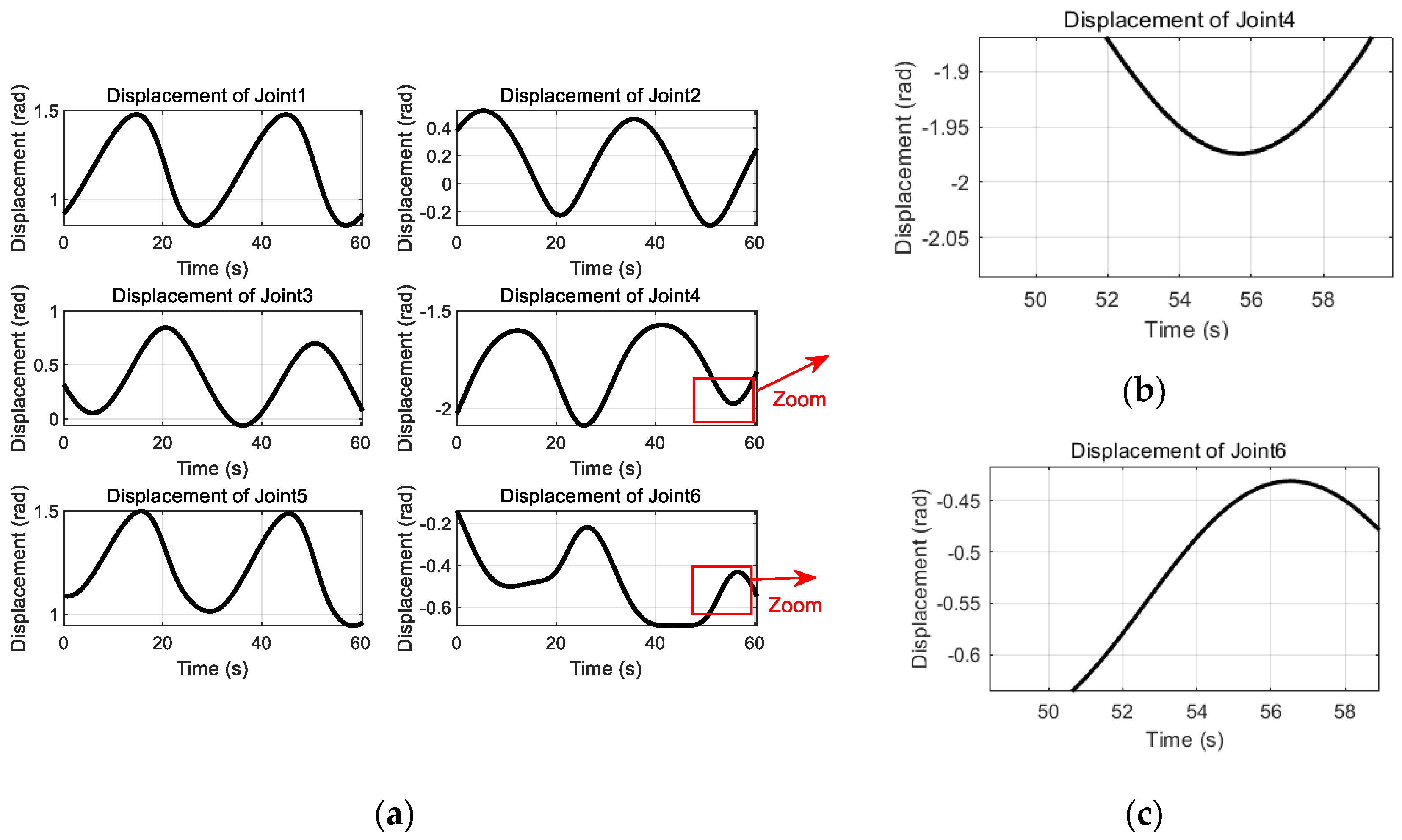
Figure 7 shows the trajectory plots of each joint of the robot achieved by using the quintic B-spline interpolation algorithm.

Figure 7a displays the displacement diagrams of the robot’s six joints, which were obtained using the quintic B-spline interpolation algorithm. In Figure 7b, by zooming in on a specific segment of joint 4’s displacement, we can observe the remarkable level of detail in the joint trajectory planning. The curve exhibits an exceptional degree of smoothness, devoid of any jagged edges or abrupt changes that could potentially compromise the robot’s performance. This high level of precision ensures that the joint movements are not only accurate but also fluid, contributing significantly to the robot’s overall effectiveness and responsiveness.

Similarly, Figure 7c, which focuses on a portion of joint 6’s displacement, also demonstrates the smoothness of the curve, further reinforcing the advantages of the B-spline approach. The seamless transition between displacement points, without any abrupt changes or distortions, showcases the algorithm’s ability to generate highly accurate and predictable motion trajectories. This is crucial for effective robot trajectory planning.

Furthermore, the B-spline interpolation algorithm’s adaptability and flexibility make it an ideal choice for handling complex robot motions. Its ability to approximate curves with high accuracy and minimal computational overhead allows for real-time implementation, enabling robots to quickly respond to changes in their environment or adjust their movements on the fly [23]. This capability is essential for robots operating in dynamic and unpredictable environments, where swift decision-making and precise execution are of utmost importance.

In conclusion, the displacement diagrams presented in Figure 7, particularly the zoomed-in views of joints 4 and 6, serve as compelling evidence of the superiority of the B-spline interpolation algorithm in achieving superior interpolation effects and generating smooth, predictable motion profiles for robotic systems.

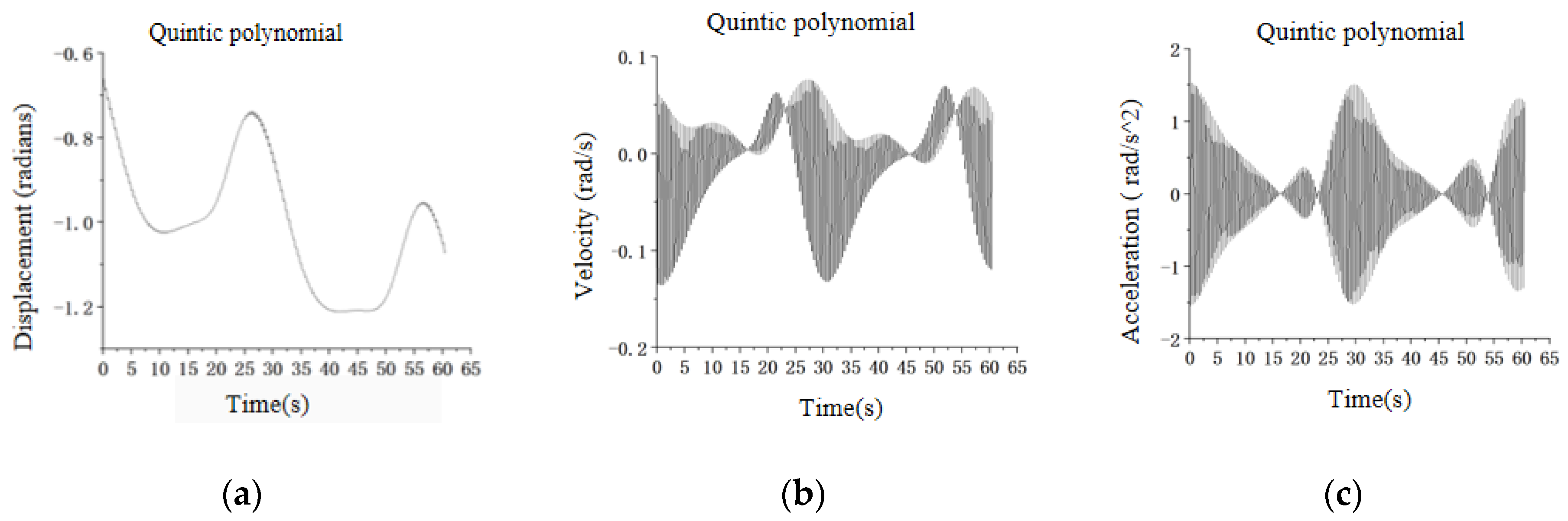
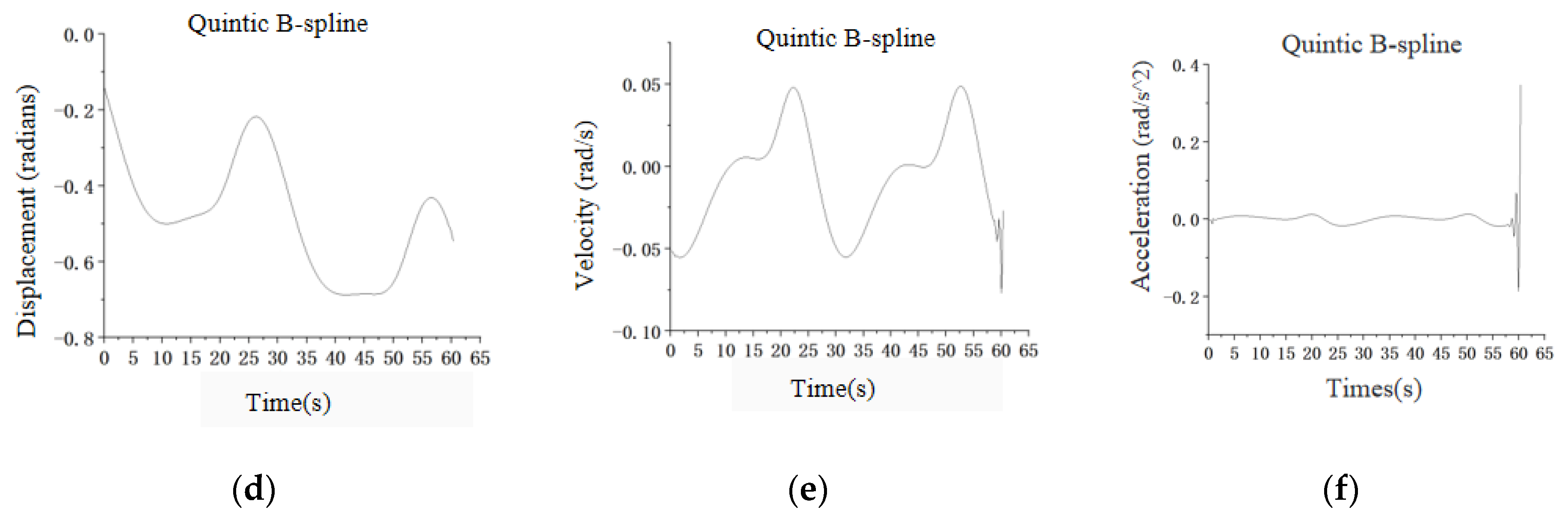
Using the B-spline interpolation algorithm, taking joint 6 as an example, the simulation curves of joint displacement, angular velocity, and angular acceleration are obtained through MATLAB programming, as shown in Figure 8d–f.

3. Comparison of Trajectory Planning Between Quintic Polynomial Interpolation Algorithm and Quintic B-Spline Interpolation Algorithm

To accurately capture the dynamics of each robotic joint, MATLAB was used as the primary tool to compute the crucial kinematic parameters: angular displacement, angular velocity, and angular acceleration. These computations are essential for understanding the behavior of the robotic system and ensuring smooth, predictable movements. We utilized line charts to depict the relationships between these variables and time, providing a clear and Intuitive representation of the data trends.

We focused on comparing the performance of two interpolation methods: the conventional fifth-degree polynomial interpolation and the more advanced fifth-degree B-spline interpolation algorithm. To illustrate the differences, we chose joint 6 as a representative example and plotted its angular displacement, angular velocity, and angular acceleration over time for both interpolation methods, as shown in Figure 8.

The simulated curve graphs in Figure 8a–c represent the joint displacement, angular velocity, and angular acceleration of joint 6, which were obtained using MATLAB programming with a quintic polynomial interpolation algorithm.

Figure 8 presents a detailed comparison of two interpolation techniques, highlighting notable differences in the motion trajectories’ smoothness and continuity. The quintic B-spline interpolation algorithm notably provides a smoother and more natural motion profile for joint 6, affecting its angular displacement, velocity, and acceleration. This superior performance is attributed to the B-spline curves’ inherent smoothness and local control capabilities, allowing precise motion adjustments and reducing oscillations or discontinuities.

Consequently, we chose the quintic B-spline interpolation algorithm for planning the spiral arc grinding trajectory, enhancing the robotic system’s precision, reducing vibrations, and boosting overall performance. With these benefits, B-spline interpolation is ideal for complex, high-precision tasks, improving the robotic grinding process’s reliability and efficiency. Regarding the robot’s movement, the end-effector maintains a constant speed, ensuring consistent time intervals between consecutive nodes. With a radius of 100 mm and a pitch of 60 mm, we calculated an initial inclination angle of φ₀ = 0.0952 and a maximum step angle of α_c ≤ 0.089. The spatial segmentation includes 71 nodes, with a set velocity of 2 mm/s along the z-axis, resulting in a time of 0.4258 s between nodes. 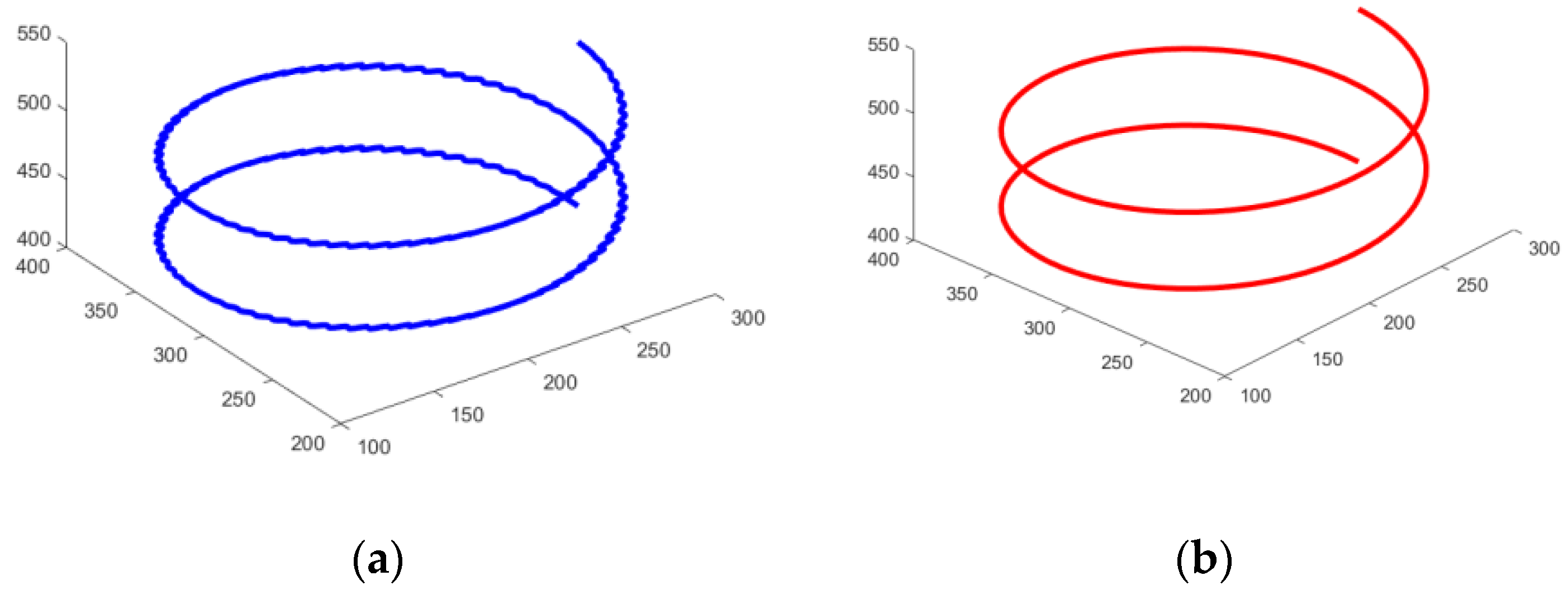Figure 9 shows the corresponding end position values of the robot.

As shown in Figure 8 and Figure 9, it becomes evident that the adoption of the quintic B-spline interpolation algorithm for trajectory planning yields significant advantages in terms of smoothness and stability. Specifically, Figure 8 not only showcases the joint trajectory but also underscores the remarkable smoothness in the profiles of joint velocity and acceleration along the trajectory. This absence of any sharp or abrupt changes is crucial as it ensures that the robot’s movements are not only precise but also free from any jarring motions that could potentially damage the mechanical components or compromise the accuracy of the task being performed.

Furthermore, the visualization in Figure 9 underscores the effectiveness of utilizing B-spline interpolation for trajectory planning by demonstrating the smooth and continuous motion path traced by the robot’s end-effector. This seamless progression, devoid of any jerky movements, underscores the robustness and reliability of the planning method. The end position values presented in this figure serve as concrete evidence that the trajectory is not only well defined but also accurately executed, underscoring the high degree of control and predictability achieved through this approach.

Additionally, the smooth motion trajectories generated by the B-spline interpolation algorithm are particularly advantageous in applications requiring precise and delicate manipulation, such as in surgical robotics, where even the slightest deviation or instability can have significant consequences. By ensuring that the robot moves smoothly and without any large vibrations, the use of this interpolation technique significantly enhances the safety and effectiveness of such operations. Thus, we believe that integrating the quintic B-spline interpolation algorithm into trajectory planning strategies serves as a valuable tool for achieving smooth and stable robot movements. As demonstrated in Figure 8 and Figure 9, this approach not only ensures precision in the execution of complex trajectories but also minimizes the risk of mechanical stress and wear, thereby enhancing the overall performance and longevity of the robotic system.

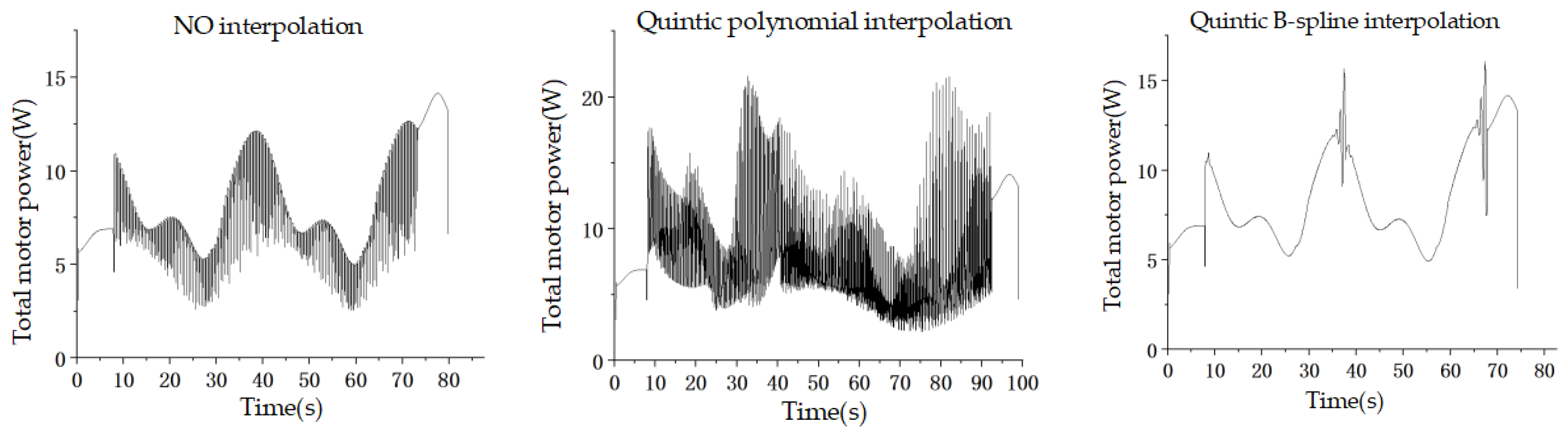
Moreover, the calculated MATLAB data were used to simulate the planning of a spatial spiral curve path for a space station polishing operation in RobotStudio 6.08, comparing three methods: no interpolation, quintic polynomial interpolation, and quintic B-spline interpolation. Enabling the simulation signal monitor in RobotStudio software, set up the signal monitor to record the total motor power and cumulative motor energy. Export the total motor power and cumulative motor energy for each of the three scenarios. Using Origin as an analytical tool, these data are processed and plotted on line charts as shown in Figure 10 and Figure 11. Figure 10 compares the energy consumption of three interpolation methods: no interpolation, quintic polynomial, and quintic B-spline interpolation. It is observed that no interpolation consumes the least power, highlighting its efficiency despite the potential compromise in motion smoothness. Quintic polynomial interpolation, while providing smoother trajectories, requires significantly more power due to frequent dynamic adjustments in motor control. In contrast, quintic B-spline interpolation offers a balance, showing moderated energy consumption with improved trajectory smoothness. 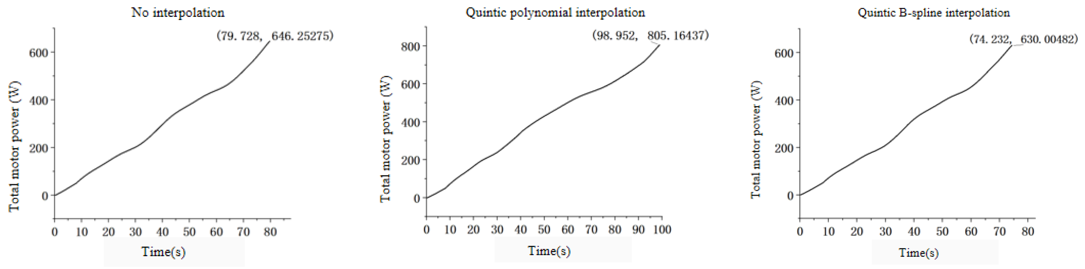The data from Figure 11 shows that the energy consumption of the no-interpolation and quintic B-spline interpolation methods are comparable, highlighting that the advanced quintic B-spline interpolation achieves enhanced motion smoothness and accuracy without significantly increasing energy use compared to simpler or no-interpolation methods. This underscores the quintic B-spline’s advantage of optimizing motion control while maintaining energy efficiency, making it an ideal choice for precision-demanding applications where both factors are crucial. In addition, we introduce a concise quantitative comparison for Figure 10 and Figure 11 for clear evaluation: (1) No Interpolation: The total energy consumption for the no-interpolation method is 646.25275 watt-hours, which reflects the most energy-efficient approach among the three methods evaluated; (2) Quintic polynomial interpolation: This method shows the highest energy consumption at 805.16337 watt-hours, indicating that while it may offer smoother trajectories, it does so at the cost of higher energy use. (3) Quintic B-spline interpolation: The energy consumption for the quintic B-spline method is 630.00482 watt-hours, positioning it as slightly more energy-efficient than the no-interpolation method, while potentially offering better control and smoothness in trajectory planning.

From the comprehensive analysis of the graphical results, it becomes evident that when tasked with grinding a consistent spatial spiral curve, the quintic polynomial interpolation algorithm, while effective, exhibits certain limitations. Specifically, it necessitates the longest execution time, indicating a less efficient trajectory planning process. Furthermore, the total motor power curve exhibits the most pronounced fluctuations, suggesting that the robot’s motor system is subjected to increased stress and potentially higher wear rates. Consequently, this algorithm consumes the greatest amount of total motor energy, impacting operational costs and potentially reducing the robot’s overall energy efficiency.

In contrast, the quintic B-spline interpolation algorithm emerges as the optimal choice for this specific application. By consuming the least amount of time for trajectory planning, it significantly enhances the robot’s productivity and response speed. Moreover, the smooth variation in the total motor power curve demonstrates the algorithm’s capability to minimize stress on the motor system, promoting longer component lifespans and reduced maintenance requirements. This smoothness also translates into reduced energy consumption, making the robot’s operation more environmentally sustainable and cost-effective.

The planning effect of not using interpolation falls between the two algorithms. While this approach may suffice for certain applications with less stringent requirements, it fails to match the efficiency and precision offered by the quintic B-spline interpolation algorithm.

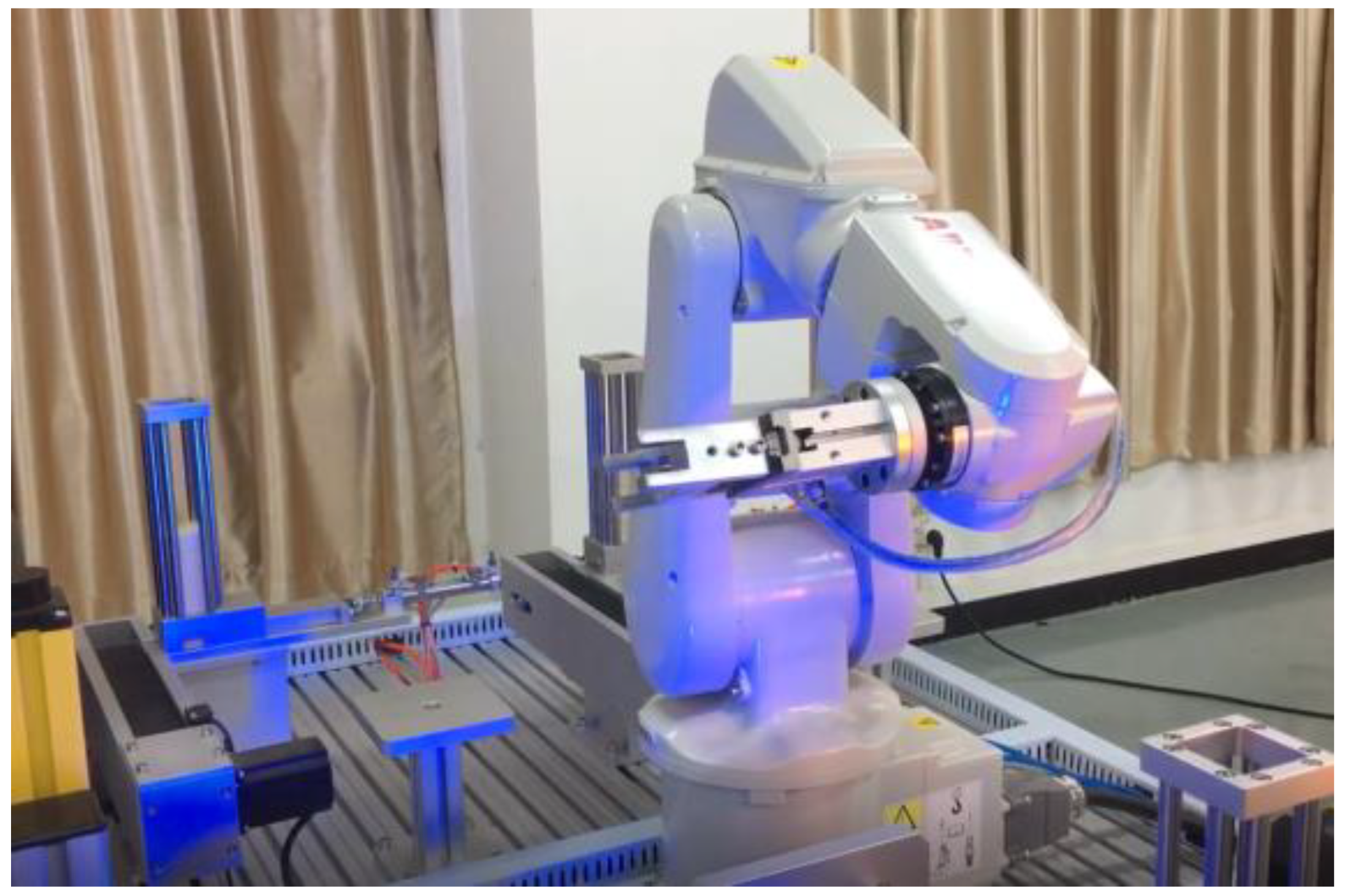
When the trajectory planning program derived from the B-spline interpolation algorithm is integrated into the robot experimental platform, the results are truly remarkable. The robot seamlessly follows the planned trajectory, executing the grinding task with stability and precision. Figure 12 is a diagram demonstrating the robot’s operation, which vividly illustrates the robot’s smooth and vibration-free operation and serves as a testament to the algorithm’s effectiveness.

In conclusion, the adoption of the quintic B-spline interpolation algorithm for trajectory planning of robots engaged in spatial spiral curve grinding offers a trifecta of benefits: a shortened running time, reduced energy consumption, and the elimination of vibrations. These advantages not only elevate the robot’s performance but also contribute to a more sustainable and cost-effective manufacturing process.

While our study focused exclusively on a spiral trajectory, we chose this due to its complexity and relevance in precision-demanding applications such as 3D printing and robotic assembly. To substantiate the choice and effectiveness of the interpolation methods used—quintic polynomial and B-spline—across various trajectory types, we refer to several studies that have successfully applied these techniques in broader contexts. For instance, Ref. [24] demonstrates the efficacy of B-spline interpolation in creating smooth and precise trajectories for industrial robots. Similarly, quintic polynomial interpolation’s applicability and benefits across different trajectory shapes are well documented [25]. These references underscore the robustness and versatility of the interpolation methods utilized in our study, supporting their effectiveness beyond the specific case of spiral trajectories examined. Although our paper currently presents results for a single trajectory type, the foundational principles and previous successful applications of these interpolation techniques reinforce the validity of our approach and findings within a broader context.

4. Conclusions

In this study, the application of quintic B-spline interpolation for spiral arc curve trajectory planning in robotic systems was demonstrated to effectively enhance motion smoothness and stability across various robot joints, leading to significantly improved performance outcomes. Our results validate that this method not only minimizes energy consumption but also effectively eliminates robot jitter, thereby enhancing the efficiency of robot trajectory planning. The quintic B-spline approach has proven to be a robust solution for maintaining high precision in complex tasks without compromising energy efficiency. Future work will continue to optimize this approach by focusing on reducing execution time, minimizing wear on robot joints to extend their lifespan, and enhancing obstacle avoidance capabilities. Additionally, integrating advanced sensing technologies such as vision systems and force sensors will enable dynamic adjustments to the trajectory in response to real-time environmental feedback, further ensuring task success under variable conditions. This comprehensive approach promises to significantly advance the field of robotic trajectory planning, particularly for precision-demanding tasks like robot grinding.