Abstract
The split delivery vehicle routing problem (SDVRP) is a relaxed variant of the capacitated vehicle routing problem (CVRP) where the restriction that each customer is visited precisely once is removed. Compared with CVRP, the SDVRP allows a reduction in the total cost of the routes traveled by vehicles. The exact methods to solve the SDVRP are computationally expensive. Moreover, the complexity and difficult implementation of the state-of-the-art heuristic approaches hinder their application in real-life scenarios of the SDVRP. In this paper, we propose an easily understandable and effective approach to solve the SDVPR based on an a priori adaptive splitting algorithm (AASA) that improves the existing state of the art on a priori split strategy in terms of both solution accuracy and time complexity. In this approach, the demand of the customers is split into smaller demand values using a splitting rule in advance. Consequently, the original SDVRP instance is converted to a CVRP instance which is solved using an existing CVRP solver. While the proposed a priori splitting rule in the literature is fixed for all customers regardless of their demand and location, we suggest an adaptive splitting rule that takes into account the distance of the customers to the depot and their demand values. Our experiments show that AASA can generate solutions comparable to the state of the art, but much faster.
1. Introduction
The split delivery vehicle routing problem (SDVRP) introduced by [1] is a relaxation of the traditional capacitated vehicle routing problem (CVRP), where each customer can be visited more than once. In both CVRP and SDVRP, a number of identical vehicles having limited capacity serve a set of customers with given demands. The vehicles depart a depot and return to the depot after visiting customers. The pairwise travel costs between customers and between customers and the depot are given. The objective is to minimize the total travel cost of the vehicles. The difference between CVRP and SDVRP is that in contrast to CVRP, where each customer is required to be visited once and by only one vehicle, SDVRP allows multiple visits to a customer. Therefore, the demand of a customer may be split among multiple vehicles. The authors in [2] showed that splitting the customer demands potentially reduces the total cost by up to . Furthermore, they show that there always exists an optimal solution to the SDVRP in which there is no k-split cycle and no two routes have more than one common customer.
Apart from environmental benefits, such as reduced emissions and energy efficiency, by allowing split deliveries, SDVRP can reduce the total distance traveled and the number of vehicles required. This optimization leads to lower fuel consumption, reduced vehicle wear and tear, and decreased maintenance costs. For businesses with large delivery fleets, these savings can be substantial. Split delivery may reduce labor, inventory, and storage costs as efficient routing reduces the time drivers spend on the road, which translates to lower labor costs. Reduced travel time also minimizes overtime and improves overall productivity. Moreover, split deliveries enable better alignment with demand patterns. By avoiding the need to stockpile large quantities of inventory, businesses can reduce warehousing costs and minimize the risk of overstocking or obsolescence. These findings justify the essence of formulating and solving the SDVRP.
State-of-the-art research has applied the SDVRP to various practical scenarios. For instance, Mullaseril et al. [3] addressed the problem of distributing feed to cattle on a large ranch in Arizona, where inaccuracies in feed loading necessitate split deliveries. Their approach, modeled as a capacitated rural postman problem with time windows, demonstrated that allowing split deliveries significantly reduced the total distance traveled by the fleet in most cases. Sierksma and Tijssen [4] studied the crew exchange process between offshore gas platforms in the North Sea. They formulated this as a discrete split delivery routing problem and employed integer programming with column generation and a cluster-and-route procedure. Their experiments showed that while their column generation approach (CGRP) was more accurate, the cluster-and-route (CR) method offered faster computation times. Song et al. [5] explored the distribution of newspapers from printing plants to agents in South Korea. They implemented a two-phase solution procedure, including agent allocation and split delivery scheduling, which improved the overall delivery efficiency and reduced costs by 15% compared to manual methods. More recently, within the context of waste management, ref. [6] utilized the SDVRP framework to model and solve complex waste collection and transportation challenges, incorporating realistic collection policies and offering insights into optimizing operational costs and fleet management, where they showed how an appropriate collection policy can significantly reduce fleet operating costs by 40–60% and fleet size by approximately 50% without causing overflow.
The SDVRP is known to be an NP-hard problem [7]. Therefore, exact solutions are only applicable to the SDVRP instances of smaller scale. Such methods typically formulate the SDVRP as a mixed integer linear program (MILP) [8] and propose different variants of branching algorithms such as branch-and-cut [9,10], branch-and-price [11,12], and branch-and-price-and-cut [13,14] for various versions of the SDVRP. However, with increasing the size of the problem, the corresponding MILP models will soon become intractable for exact solutions. To tackle this issue, various traditional approximation techniques, heuristics and metaheuristics have been proposed to deal with the high time-complexity of the large SDVRP models. For instance, a max–min clustering before solving the optimization problem is proposed in [15]. Tabu search has been used in several papers [16,17,18]. In [16], the authors proposed an approach relying on simulated annealing to solve the SDVRP. Other lines of research propose methods utilizing ant colony optimization [19,20], genetic algorithms [21,22], and particle swarm optimization [23,24], to solve the SDVRP. Using column generation is another optimization technique that has been applied to the SDVRP by [8,25]. The authors in [26] applied the cutting plane method to tackle the time complexity of the SDVRP.
Recently, the authors in [27] introduced a metaheuristic approach incorporating several mathematical programming components within an iterative local search framework. We refer to this method as ILS-MIP in the rest of the paper. ILS-MIP starts from an initial set of solutions obtained using the I1 Solomon heuristic followed by a perturbation step (to escape local optima), a local search step using classical neighborhood search heuristics, and several steps based on hybrid components. The hybrid components are called only if the incumbent solution of the search is not improved after a number of steps. The hybrid components encompass a mixed integer program (MIP)-based improvement heuristic performing two operations of inserting splits or removing potential unnecessary splits. Another used hybrid component is based on converting the current SDVRP solution to a CVRP instance and using a hybrid genetic search (HGS) framework [28] specialized to solve a CVRP. An MIP model is also used in the third component of the hybrid step where a residual problem is constructed by removing the edges that are not used in any solution of the current set of solutions. The residual problem is then solved using an MIP solver. Finally, the fourth component uses the branch-and-cut (BC) framework proposed in [29]. While ILS-MIP is a powerful and effective methodology, its complexity and significant runtime for larger instances makes it challenging for addressing real-world problems.
Although the state-of-the-art algorithms for the SDVRP are known for their ability to produce high-quality solutions, they often pose challenges in terms of complexity and practical implementation. In response to these challenges, the authors in [30] introduced an efficient algorithm that decomposes the SDVRP into two sub-problems. First, a demand-splitting rule is applied to all customers. The idea of splitting the customer demands was introduced in [31]; the authors propose a heuristic solution for SDVRP with time windows based on the column generation approach. In this paper, it is assumed that the demand of each customer is served by a number of orders selected from a set of feasible orders where each order is a pre-determined discrete split of the customer demand. The authors in [30] proposed applying the a priori splitting strategy in which the demand of each customer is split into smaller demands, each representing a new customer located in the same position as the original customer. As a result, a new problem instance is generated with an increased number of customers. Second, the new problem is assumed to be an instance of the CVRP which is solved using existing powerful CVRP solvers. The transformation of the SDVRP to a CVRP not only facilitates the implementation of SDVRP but also enables leveraging the rich literature on the CVRP. The obtained solution for the resulting CVRP is then translated back to the original SDVRP.
Regarding the splitting strategy, the solutions proposed in both [30,31] are based on a static splitting rule without taking into account the specific characteristics of the problem, such as customers’ location and demand. In the method proposed by [30], a fixed splitting rule that is inspired by the US coin denominations is applied to all customer demands and the VRPH solver introduced by [32] is used to solve the resulting CVRP instance. We refer to this algorithm as VRPHAS in the rest of this paper. The numerical evaluation of VRPHAS illustrates its ability to produce acceptable sub-optimal solutions in much less time compared to the state-of-the-art heuristic algorithms. However, the adoption of the introduced splitting rule is not well justified. Instead of applying a fixed rule to all customers, a splitting rule that is adaptive, based on the specific characteristics of a customer can potentially result in an improved solution for the SDVRP. In this paper, we study the problem of defining a good splitting rule for each customer. To this end, we introduce an a priori adaptive splitting algorithm (AASA). In combination with the VRPH solver, AASA results in an improved performance in terms of the optimality gap without significantly increasing the computational complexity of VRPHAS. AASA achieves this by taking into account the distance between the customers and the depot, the value of the customers’ demand along with the vehicles’ capacity. Similar to VRPHAS, AASA can be used with any CVRP solver. Thus, it provides a method to solve the SDVRP that is easily understandable, can be implemented simply, and generates high-quality solutions very quickly.
The rest of the paper is organized as follows. In Section 2.1, we provide a formal definition of the SDVRP. Our proposed solution is explained in Section 2.2. Section 3 presents the numerical results. Finally, the conclusion is discussed in Section 4.
2. Problem Definition and the Proposed Solution
2.1. SDVRP Definition
Let denote an undirected and weighted complete graph representing the network of customers and a depot. The vertex set represents the depot denoted by the vertex 0 and n customers indexed as . A non-negative weight is associated with each edge of the graph that stands for the cost of traveling between customers i and j. Moreover, each customer has a positive demand, denoted by . A set of M vehicles is available to serve the customers’ demands. Each vehicle has a limited capacity denoted by Q. The objective of the SDVRP is to find a route for each vehicle such that the demands of all customers are satisfied with the minimum total cost. In this paper, we assume that the cost of traveling between customers is their Euclidean distance denoted by the function , i.e., .
2.2. Proposed Heuristic Algorithm for SDVRP
In the following, we first describe the idea of the a priori splitting rule proposed by [30] and then discuss the core algorithmic idea of AASA based on two motivational observations. We then formalize AASA in detail.
A Priori Splitting Rule
The proposed splitting rule in [30] is inspired by the US coin denominations. The authors propose two splitting options , and . The first option replaces customer i, with the demand of , by , , and customers with the demand values of , , and , respectively. Hence, we have:
A similar breakdown can be given for the second splitting rule option. Using the splitting rule , the demand of customer i is split into smaller values. The customer i is then replaced by customers located at the same position as customer i and with the demand values resulting from (1)–(4). After applying the splitting rule to all customers, a new graph is constructed with vertices (customers). The new graph is considered as an instance of the CVRP and the VRPH solver is used to solve it. The resulting solution is also a solution to the original SDVRP instance. In the next section, we justify the essence of the adaptation of the splitting rule and propose the AASA algorithm.
2.3. A Priori Adaptive Splitting Algorithm (AASA)
The a priori splitting rule described by Equations (1)–(4) is a fixed rule, i.e., a single splitting rule is applied to all customers regardless of their demand and location. However, the information regarding the customers’ demand and location can be leveraged in the vehicle routing decisions towards reducing the total travel cost as well as the size of the resulting CVRP instance. We propose an adaptive splitting rule based on the location and demand information that is shown to effectively improve the solution. In the following, we first present the motivation behind the main building blocks of our proposed splitting rule. We then explain the AASA algorithm.
2.3.1. Motivation
In this section, we present the motivation behind our proposed splitting algorithm through illustrative examples. We study the impact of the splitting rule granularity on the total travel cost and the solution runtime considering customers’ demand values and their distances from the depot. Our investigations reveal the benefits of using coarser/finer splitting rules for different customers depending on their demand and location. By a coarser splitting rule, we mean one that entails larger splitting portions as opposed to a finer splitting rule where the portions are smaller. For instance, for a demand point with , the splitting rule is coarser compared to the rule .
Impact of coarser rules for customers with higher demands: Using coarser rules for customers with high demands introduces a two-fold benefit: (i) it reduces the runtime due to a smaller number of resulting customers in the resulting CVRP and (ii) it often results in a lower total cost of delivery. To capture this effect, we employ an exponential pattern (such as 128/64/32/16/8/4/2) for the AASA rule. We illustrate this effect for the instance of the third dataset provided in [33], as depicted in Figure 1. In this instance, the vehicle capacity is 200 and the depot is located at the location in Figure 1a,b. Each point in the plane corresponds to a customer. The routes of the vehicles in the obtained solution are denoted by different colors. Figure 1a,b show the solution of the SDVRP instance considering the and splitting rules, respectively. We observe that the splitting rule of reduces the solver runtime by an order of . The lower runtime is expected since using an exponential pattern in the splitting rule results in splitting the higher demands into a piece with a very high value and most likely fewer pieces in total. This effect can also be observed from the size of the generated CVRP instance. The rule resulted in a new instance with 855 customers (nodes), while the rule generated a network with 572 customers. Moreover, the coarser splitting rule of resulted in a cost of that improves upon the cost of the rule (proposed by the VRPHAS algorithm) by .
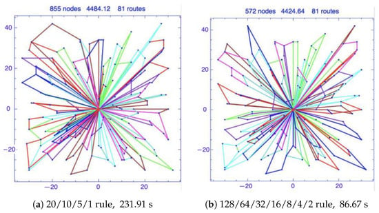
Figure 1.
Impact of using splitting rules with different granularity for different demands.
Impact of coarser rules for customers further away from the depot: The second motivation behind our proposed AASA rule is that using coarser rules for the demands with a larger distance from the depot and splitting closer demands into smaller pieces results in lower solver runtime and possibly a better solution. The intuition behind this observation is that as the distance between a customer and the depot increases, each visit to that customer would significantly increase the cost. Therefore, it is desirable to satisfy the demand of further customers within the fewest possible number of visits and that is only possible by applying coarser splitting rules to those nodes. Moreover, by splitting closer-to-depot customer demands into smaller pieces, we provide the opportunity for the vehicles returning to the depot to utilize their remaining capacity to fulfill smaller demands and, therefore, minimize the fraction of their unused capacity. It is important to note that all of these intuitive statements are based on the fact that after splitting demands and generating a new network with a larger number of customers, we use the VRPH solver and basically solve the generated instance by a number of heuristic and metaheuristic methods. Figure 2a–c illustrate the above observation for the instance from [34]. The best-known solution for this instance is . In Figure 2a,b, the results of using the and rules are shown. Although these two rules alone provide acceptable results with the costs of and , respectively, we observe that by using a combination of the two rules as shown in Figure 2c, we can achieve lower cost of . In this experiment, the 32 customers are clustered into two categories of size 16. For the 16 customers closer to the depot, we used the splitting rule , and the coarser splitting rule is applied to the remaining 16 customers located farthest from the depot.
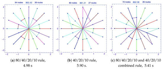
Figure 2.
Impact of using splitting rules with different granularity according to the customers’ distance to the depot.
2.3.2. AASA Algorithm
The above observations highlight the significance of applying an adaptive splitting rule for different customers instead of using a fixed splitting rule for all customers, as in VRPHAS. Motivated by these observations, we incorporate the following factors into AASA:
- Vehicle capacity: As implied by [30], it makes sense to look for the splitting rule as a function of the vehicle capacity. This not only presents a structured representation with vehicle capacity as the kernel allowing for better generalization but also leads the policy towards leaving the lowest portion of the vehicles’ capacities unused, and consequently, increases the vehicles’ utilization.
- Customer location: We believe one potential improvement to the VRPHAS splitting rule is to personalize the rule for each customer considering its distance from the depot. We observe that if the customers that are located further from the depot are visited by one (or very few) vehicle(s), the total travel cost is lower. Otherwise, if a long distance needs to be traversed multiple times, the cost will be negatively impacted. This can be avoided by coarsening the splitting rule for further customers. In AASA, the impact of customers’ locations is addressed by partitioning the customers into a number of clusters based on their distance from the depot. We then use a different splitting rule for each cluster. A coarser splitting rule is used for clusters of customers further from the depot while finer rules are applied to the clusters closer to the depot.
- Customer demand: Another important factor in the adaptation of the splitting rule is the demand of customers. Depending on how large the demand is, the splitting rule can be applied in full or partially to result in an appropriate number of additional demand points with appropriate demand values. In order to create the exponential pattern in the splitting rule, we propose to decompose the customers’ demands based on the different powers of prime numbers. For instance, the demand of a customer with served by vehicles with capacity can be decomposed as if , and if .
Leveraging the above factors, the AASA solution framework is shown in Figure 3. First, AASA employs a clustering algorithm to partition the customers into multiple levels. In our experiments, we used a simple distance-based clustering as follows:
where L is the number of levels, and is the maximum customer–depot distance among all customers, i.e, . As a result of this clustering rule, first, the customers are separated with L uniformly spaced rings around the depot. Second, for the customers at each level, the same splitting rule is applied. After all the demands are split, a CVRP instance is generated. Finally, the VRPH solver is used to solve the resulting CVRP instance.

Figure 3.
AASA framework.
The pseudo-code for AASA is given in Algorithm 1. The algorithm starts by taking as input the SDVRP instance as a graph , the vehicle capacity Q, the vector of customer–depot distances denoted by where , and the vector of customer demands . Next, it computes d, the greatest common divisor () of the demands vector and the vehicle capacity, which will be used as a parameter in the adaptive splitting rule. The vehicles may carry goods only in quantities that are multiples of d units. This is to control the granularity of the splitting rule. Next, the demand vector is scaled down by d and averaged over the customers to find that is used in finding determining the largest quantity of goods that is demanded by the customers in the equivalent CVRP model.
| Algorithm 1 A priori Adaptive Splitting Algorithm (AASA) |
Input: Output:
|
The algorithm takes into account L different levels for the distance-based clustering as provided in (5). Then, for each level i, the splitting rule is determined using the value . Next, the clustering of the customers is made according to Equation (5). The split function substitutes each node (customer) of the graph G with new customers according to the rule to gradually form the graph . Note that the splitting rule ensures that the demands further away from the depot are split with coarser rules. Once the graph is completed, the CVRP solver will solve the generated new problem. We experimented with different values of the prime number p and observed that has the best performance overall in the current version of AASA.
For example, consider the instance from SET-1 as shown in Figure 2. We will have , i.e., . The simple distance-based clustering in Equation (5) with results in two levels, where covers the customers that are furthest from the depot and covers the customers that are closest to the depot. We will have and . Therefore, for the first level, we have and for .
VRPH solver: Once the a priori splitting rule is applied to an SDVRP problem, any commercial solver can be used to solve the resulting CVRP instance. In this paper, we use the VRPH solver to solve CVRP instances. VRPH is a publicly available solver with a provable record of generating high-quality solutions. It takes as input a CVRP instance written to a file with a format similar to that of the Traveling Salesman Problem Library (TSPLIB) files and prints the solution to an output file. VRPH implements an open-source library of several local search heuristics for generating and improving feasible solutions to the CVRP instances. We refer the reader to [35] for a detailed description of the heuristics and the modular structure of the VRPH software. In this paper, we use VRPH as a standalone solver with the parameters set at their default values.
3. Performance Evaluation
In this section, we evaluate the performance of AASA through extensive numerical simulations. We benchmark the performance of AASA against three baseline strategies, using instances from datasets that are widely used in the literature for the comparison of various vehicle routing solutions. Table 1 presents the summary of the evaluation datasets used throughout this section. Further details about the instances of each dataset are provided in Section 3.1.

Table 1.
Evaluation datasets.
3.1. Benchmarking Instances
We consider 4 benchmarking sets that include 88 instances overall as presented in Table 1. SET-1 [34] contains 21 instances, each with customers uniformly distributed on the perimeter of concentric circles centered at the depot. The instances are sorted by the number of customers and the number of concentric circles. SET-2 [36] and SET-3 [33] instances use similar customer demand profiles but vary in the number of customers and vehicle capacity. These demands are randomly sampled from the range with chosen by six different scenarios as in Table 1. SET-2 contains 14 and SET-3 contains 42 instances, 6 of which are repeated. Therefore, we test only the 36 of them that are not redundant. The coordinates of the customers in SET-2 are randomly generated using the coordinates of eil51, eil76, and eil101 from TSPLIB, which are also used in SET-4 [37]. SET-4 includes 11 instances where no specific rule is preserved throughout for generating the customer demands.
3.2. Benchmarking Solutions
We benchmark the performance of the AASA algorithm against the following baseline methods:
- No-splitting (CVRP): The baseline method that treats an SDVRP instance as a CVRP instance and runs the VRPH [32] solver to generate solutions.
- VRPHAS: The method based on a priori splitting that is proposed by [30].
- ILS-MIP: The metaheuristic method proposed by [27].
We note that when computing the optimality gap corresponding to each method for each experimental instance, we take the best solution known in the literature as the reference solution. Furthermore, we note that in ILS-MIP, the travel cost between each pair of customers is assumed to be their rounded Euclidean distance except for SET-1 instances where the exact Euclidean distance is taken as the cost. Hence, we compare the results of ILS-MIP and AASA only for SET-1. For the rest of the datasets, we compare the performance of AASA against the No-splitting and the VRPHS methods.
3.3. Metrics and Setup
We consider the optimality gap and the solver runtime as metrics for performance comparison between the above strategies. The optimality gap which indicates the deviation from the best-known solution is defined as:
where is the objective value of the considered method. We run both VRPHAS and AASA algorithms on the same PC with an Intel Xeon processor at GHz and 16 GB of main memory. It is important to note that the gap results we obtained for the VRPHAS method do not match the values presented in [30] for some instances. However, since we need to compare both the runtime and the gap results for the VRPHAS and AASA methods on similar hardware, we reflect the results of our run for VRPHAS. Moreover, we report the computation time of the ILS-MIP method presented in [27], including the values of time and corresponding to the time required for the proposed iterative algorithm to terminate and the time at which the best solution of ILS-MIP is achieved, respectively. A time limit (TL) is considered for the algorithm termination that is assumed to be equal to 1349 s by [27]. It is important to note that the ILS experiments are conducted on a PC with an Intel Core i7-8700 3.2 GHz processor and 32 GB of memory which is more powerful than our PC. Therefore, we can expect that ILS-MIP performs even worse in terms of computation time compared to AASA if both were run on the same hardware.
3.4. Numerical Results
3.4.1. CVRP Instance Attributes Comparison: AASA vs. VRPHAS
As illustrated in Section 2.3.1, one of the promises of our proposed splitting algorithm is generating smaller size CVRP instances that can be solved consistently faster. To show this, we present the size of the CVRP instances and the number of routes (i.e., vehicles) in the generated CVRP solution obtained by the splitting strategies of VRPHAS and AASA for the evaluation sets SET-1 to SET-4 in Table 2, Table 3, Table 4 and Table 5, respectively. It is observed that for all the benchmarking datasets, AASA reduces the size of the CVRP problem compared to the VRPHAS method. Moreover, the number of routes in the solution obtained by AASA is less than or equal to the VRPHAS solution except for a few instances. Although the reduced number of routes indicates the potential of AASA in producing better solutions compared to VRPHAS, it does not provide sufficient evidence for cost-efficiency since the actual routes taken by the vehicles determine the total cost. However, together with the solution gap results shown in the next section, we can conclude that AASA performs better than VRPHAS in terms of both solution quality and runtime and that is a result of the adaptive splitting approach we proposed.

Table 2.
CVRP instance attributes: VRPHAS vs. AASA on SET-1.

Table 3.
CVRP instance attributes: VRPHAS vs. AASA on SET-2.

Table 4.
CVRP instance attributes: VRPHAS vs. AASA on SET-3.

Table 5.
CVRP instance attributes: VRPHAS vs. AASA on SET-4.
3.4.2. Optimality Gap and Runtime Comparison: AASA against Baselines
Table 6 presents the performance of AASA against VRPHAS, ILS-MIP, and the no-splitting strategies for the instances of SET-1. First, we observe that the no-splitting method results in very low-quality solutions as the resulting optimality gap obtained by this method is very high compared to the VRPHAS, AASA, and ILS-MIP heuristics. Moreover, we observe that while the ILS-MIP strategy outperforms the AASA and VRPHAS solution approaches in terms of optimality gap for almost all instances of SET-1, it requires very large computation times. The average runtime for ILS-MIP is s as opposed to the average runtime of s and s corresponding to the VRPHAS and AASA solution approaches, respectively. This huge time complexity hinders the practical application of the ILS-MIP approach in real-world problems with time sensitivity or scalability requirements. Figure 4 and Figure 5 illustrate the per-instance optimality gap and runtime of our proposed splitting rule against the fixed splitting rule introduced in VRPHAS. Our proposed method outperforms the VRPHAS in terms of time complexity for all instances, and it also improves upon the average optimality gap of VRPHAS. Moreover, while the VRPHAS method results in the optimality gap in the worst-case scenario (), AASA achieves the maximum optimality gap of for the same instance. We also observe that AASA finds the best-known solution for four instances as opposed to the VRPHAS method obtaining the best-known solution for three instances of SET-1.

Table 6.
Performance of VRPHAS, AASA, and ILS-MIP on SET-1.
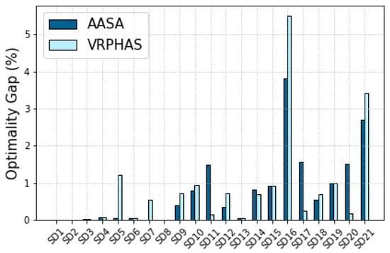
Figure 4.
Per-instance gap of SET-1.
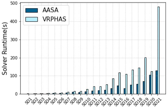
Figure 5.
Per-Instance solver runtime of SET-1.
Table 7 shows the results of VRPHAS, AASA, and the no-splitting methodologies for the instances of SET-2. According to Table 7, the no-splitting approach results in a higher gap compared to both the VRPHAS and AASA rules. Furthermore, our proposed AASA strategy outperforms the VRPHAS method in terms of the average optimality gap, as well as runtime. Moreover, the per-instance results depicted in Figure 6 and Figure 7 indicate that the AASA strategy improves upon the optimality gap and solver runtime of the VRPHAS method for almost all instances of SET-2. It can also be observed that while the VRPHAS method exhibits an optimality gap of in the worst-case scenario (), AASA achieves a maximum optimality gap of ().

Table 7.
Performance of VRPHAS, AASA, and the no-splitting methodologies on SET-2.
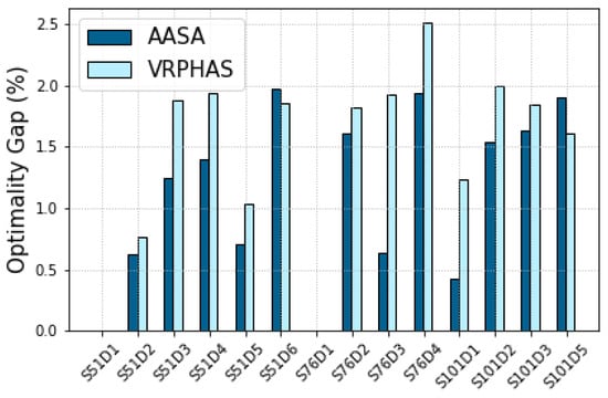
Figure 6.
Per-instance gap of SET-2.
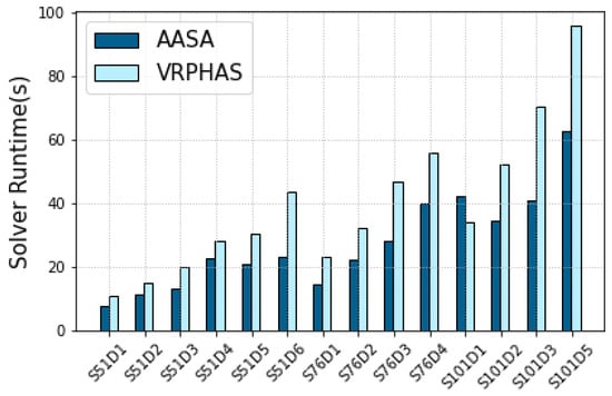
Figure 7.
Per-instance solver runtime of SET-2.
Similarly, the comparison of the results for SET-3 and SET-4 provided in Table 8 and Table 9 show that our proposed splitting algorithm again improves both average optimality gap and runtime of the VRPHAS splitting mechanism and, therefore, it can effectively generate higher-quality solutions, faster than VRPHAS. The improvement in the runtime is mainly owing to the rule granularity consideration introduced in AASA as discussed in Section 2.2, which results in smaller instances to be solved by the CVRP solver compared to the VRPHAS method. Figure 8 and Figure 9 illustrate the per-instance optimality gap and runtime of SET-3. According to Table 8 and Figure 8, although the VRPHAS method results in the maximum optimality gap of (), the worst-case optimality gap achieved by AASA is (). The optimality gap and run-time of SET-4 instances are presented in Figure 10 and Figure 11. Table 9 and Figure 10 illustrate that the AASA method improves the worst-case optimality gap of VRPHAS in SET-4, since AASA achieves the maximum optimality gap of () as opposed to the maximum gap of obtained by VRPHAS for the same instance.

Table 8.
Performance of VRPHAS, AASA, and the no-splitting methodologies on SET-3.

Table 9.
Performance of VRPHAS, AASA, and the no-splitting methodologies on SET-4.
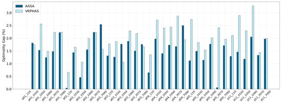
Figure 8.
Per-instance gap of SET-3.
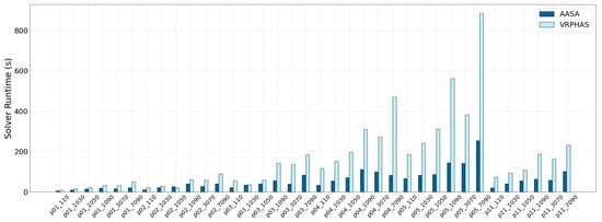
Figure 9.
Per-instance solver runtime of SET-3.
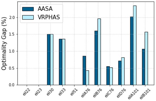
Figure 10.
Per-instance AASA gap of SET-4.
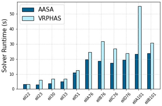
Figure 11.
Per-instance solver runtime of SET-4.
4. Conclusions
In this paper, we propose an efficient and effective heuristic algorithm for the SDVRP based on a two-step procedure of splitting the demand of customers into smaller demands and solving the generated network assuming it to be a CVRP instance. Our approach focuses on enhancing the state-of-the-art splitting rule by considering customer locations and demand values. Our proposed adaptive splitting algorithm incorporates clustering customers based on their location and choosing a specific splitting rule for each cluster. It is shown to outperform the fixed splitting rule of the approach adopted by the state of the art, for all four benchmark datasets on average, with respect to both performance and computational effort.
Author Contributions
Conceptualization, N.T., A.G., J.S.B. and B.L.G.; Methodology, N.T., A.G. and J.S.B.; Software, N.T. and A.G.; Validation, A.G. and B.L.G.; Formal analysis, N.T., A.G. and B.L.G.; Investigation, N.T. and A.G.; Resources, N.T. and A.G.; Writing – original draft, N.T., A.G. and B.L.G.; Writing – review and editing, J.S.B. and B.L.G.; Visualization, J.S.B. and B.L.G.; Supervision, J.S.B. and B.L.G.; Project administration, J.S.B.; Funding acquisition, N.T., A.G. and J.S.B. All authors have read and agreed to the published version of the manuscript.
Funding
The research of N. Torkzaban, A. Gholami, and J. Baras was partially supported by ONR grant N00014-17-1-2622, and by a grant from Lockheed Martin Chair in Systems Engineering.
Data Availability Statement
Data are contained within the article.
Conflicts of Interest
The authors declare no conflict of interest.
References
- Dror, M.; Trudeau, P. Savings by split delivery routing. Transp. Sci. 1989, 23, 141–145. [Google Scholar] [CrossRef]
- Archetti, C.; Savelsbergh, M.; Speranza, M. Worst-case analysis for split delivery vehicle routing problems. Transp. Sci. 2006, 40, 226–234. [Google Scholar] [CrossRef]
- Mullaseril, P.; Dror, M.; Leung, J. Split-delivery routing heuristics in livestock feed distribution. J. Oper. Res. Soc. 1997, 48, 107–116. [Google Scholar] [CrossRef]
- Sierksma, G.; Tijssen, G. Routing helicopters for crew exchanges on off-shore locations. Ann. Oper. Res. 1998, 76, 261–286. [Google Scholar] [CrossRef]
- Song, S.; Lee, K.; Kim, G. A practical approach to solving a newspaper logistics problem using a digital map. Comput. Ind. Eng. 2002, 43, 315–330. [Google Scholar] [CrossRef]
- Luo, K.; Zhao, W.; Zhang, R. A multi-day waste collection and transportation problem with selective collection and split delivery. Appl. Math. Model. 2024, 126, 753–771. [Google Scholar] [CrossRef]
- Archetti, C.; Feillet, D.; Gendreau, M.; Speranza, M.G. Complexity of the VRP and SDVRP. Transp. Res. Part C Emerg. Technol. 2011, 19, 741–750. [Google Scholar] [CrossRef]
- Archetti, C.; Bianchessi, N.; Speranza, M.G. A column generation approach for the split delivery vehicle routing problem. Networks 2011, 58, 241–254. [Google Scholar] [CrossRef]
- Hernández-Pérez, H.; Salazar-González, J.-J. A Branch-and-cut algorithm for the split-demand one-commodity pickup-anddelivery travelling salesman problem. Eur. J. Oper. Res. 2021, 297, 467–483. [Google Scholar] [CrossRef]
- Wolfinger, D.; Salazar-González, J.-J. The pickup and delivery problem with split loads and transshipments: A branch-and-cut solution approach. Eur. J. Oper. Res. 2020, 289, 470–484. [Google Scholar] [CrossRef]
- Casazza, M.; Ceselli, A.; Calvo, R.W. A route decomposition approach for the single commodity Split Pickup and Split Delivery Vehicle Routing Problem. Eur. J. Oper. Res. 2019, 289, 897–911. [Google Scholar] [CrossRef]
- Li, J.L.; Qin, H.; Shen, H.X.; Tong, X.; Xu, Z. Exact algorithms for the multiple depot vehicle scheduling problem with heterogeneous vehicles, split loads and toll-by-weight scheme. Comput. Ind. Eng. 2022, 168, 108137. [Google Scholar] [CrossRef]
- Li, J.; Qin, H.; Baldacci, R.; Zhu, W. Branch-and-price-and-cut for the synchronized vehicle routing problem with split delivery, proportional service time and multiple time windows. Transp. Res. Part E Logist. Transp. Rev. 2020, 140, 101955. [Google Scholar] [CrossRef]
- Gschwind, T.; Bianchessi, N.; Irnich, S. Stabilized branch-price-and-cut for the commodity-constrained split delivery vehicle routing problem. Eur. J. Oper. Res. 2019, 278, 91–104. [Google Scholar] [CrossRef]
- Min, J.N.; Jin, C.; Lu, L.J. Maximum-minimum distance clustering method for split-delivery vehicle-routing problem: Case studies and performance comparisons. Adv. Prod. Eng. Manag. 2019, 14, 125–135. [Google Scholar] [CrossRef]
- Wang, J.; Jagannathan, A.K.; Zuo, X.; Murray, C.C. Two-layer simulated annealing and tabu search heuristics for a vehicle routing problem with cross docks and split deliveries. Comput. Ind. Eng. 2017, 112, 84–98. [Google Scholar] [CrossRef]
- Xia, Y.; Fu, Z. An adaptive tabu search algorithm for the open vehicle routing problem with split deliveries by order. Wirel. Pers. Commun. 2018, 103, 595–609. [Google Scholar] [CrossRef]
- Xia, Y.; Fu, Z.; Tsai, S.B.; Wang, J. A new TS algorithm for solving low-carbon logistics vehicle routing problem with split deliveries by backpack—From a green operation perspective. Int. J. Environ. Res. Public Health 2018, 15, 949. [Google Scholar] [CrossRef] [PubMed]
- Ma, X.; Liu, C. Improved Ant Colony Algorithm for the Split Delivery Vehicle Routing Problem. Appl. Sci. 2024, 14, 5090. [Google Scholar] [CrossRef]
- Yang, W.; Wang, D.; Pang, W.; Tan, A.-H.; Zhou, Y. Goods consumed during transit in split delivery vehicle routing problems: Modeling and solution. IEEE Access 2020, 8, 110336–110350. [Google Scholar] [CrossRef]
- Jiang, Y.; Bian, B.; Liu, Y. Integrated multi-item packaging and vehicle routing with split delivery problem for fresh agri-product emergency supply at large-scale epidemic disease context. J. Traffic Transp. Eng. (Engl. Ed.) 2020, 8, 196–208. [Google Scholar] [CrossRef]
- Fan, H.M.; Zhang, X.; Ren, X.X.; Liu, P. Optimization of multi-depot open split delivery vehicle routing problem with simultaneous delivery and pick-up. Syst. Eng.-Theory Pract. 2021, 41, 1521–1534. [Google Scholar]
- Shi, J.; Zhang, J.; Wang, K.; Fang, X. Particle swarm optimization for split delivery vehicle routing problem. Asia-Pac. J. Oper. Res. 2018, 35, 1840006. [Google Scholar] [CrossRef]
- Qing, D.S.; Deng, Q.L.; Li, J.J.; Liu, S.; Liu, X.; Zeng, S.P. Split vehicle route planning with full load demand based on particle swarm optimization. J. Control Decis. 2021, 36, 1397–1406. [Google Scholar]
- Jin, M.; Liu, K.; Eksioglu, B. A column generation approach for the split delivery vehicle routing problem. Oper. Res. Lett. 2008, 36, 265–270. [Google Scholar] [CrossRef]
- Bianchessi, N.; Drexl, M.; Irnich, S. The split delivery vehicle routing problem with time windows and customer inconvenience constraints. Transp. Sci. 2019, 53, 1067–1084. [Google Scholar] [CrossRef]
- Alvarez, A.; Munari, P. A Matheuristic Approach for Split Delivery Vehicle Routing Problems. 2022. Available online: http://www.optimization-online.org/DB_FILE/2022/02/8790.pdf (accessed on 31 August 2023).
- Vidal, T. Hybrid genetic search for the CVRP: Open-source implementation and SWAP* neighborhood. Comput. Oper. Res. 2022, 140, 105643. [Google Scholar] [CrossRef]
- Munari, P.; Savelsbergh, M. Compact formulations for split delivery routing problems. Transp. Sci. 2022, 56, 1022–1043. [Google Scholar] [CrossRef]
- Chen, P.; Golden, B.; Wang, X.; Wasil, E. A novel approach to solve the split delivery vehicle routing problem. Int. Trans. Oper. Res. 2017, 24, 27–41. [Google Scholar] [CrossRef]
- Salani, M.; Vacca, I. Branch and price for the vehicle routing problem with discrete split deliveries and time windows. Eur. J. Oper. Res. 2011, 213, 470–477. [Google Scholar] [CrossRef]
- Groer, C. VRPH. 2011. Available online: https://github.com/coin-or/VRPH (accessed on 1 August 2024).
- Archetti, C.; Speranza, M.G.; Savelsbergh, M.W. An optimization-based heuristic for the split delivery vehicle routing problem. Transp. Sci. 2008, 42, 22–31. [Google Scholar] [CrossRef][Green Version]
- Chen, S.; Golden, B.; Wasil, E. The split delivery vehicle routing problem: Applications, algorithms, test problems, and computational results. Netw. Int. J. 2007, 49, 318–329. [Google Scholar] [CrossRef]
- Groer, C.S.; Golden, B.; Wasil, E. A Library of Local Search Heuristics for the Vehicle Routing Problem. Math. Program. Comput. 2010, 2, 79–101. [Google Scholar] [CrossRef]
- Belenguer, J.M.; Martinez, M.C.; Mota, E. A lower bound for the split delivery vehicle routing problem. Oper. Res. 2000, 48, 801–810. [Google Scholar] [CrossRef]
- Reinhelt, G. TSPLIB: A Library of Sample Instances for the TSP (and Related Problems) from Various Sources and of Various Types. 2014. Available online: http://comopt.ifi.uni-heidelberg.de/software/TSPLIB95 (accessed on 31 August 2023).
Disclaimer/Publisher’s Note: The statements, opinions and data contained in all publications are solely those of the individual author(s) and contributor(s) and not of MDPI and/or the editor(s). MDPI and/or the editor(s) disclaim responsibility for any injury to people or property resulting from any ideas, methods, instructions or products referred to in the content. |
© 2024 by the authors. Licensee MDPI, Basel, Switzerland. This article is an open access article distributed under the terms and conditions of the Creative Commons Attribution (CC BY) license (https://creativecommons.org/licenses/by/4.0/).