Detection and Reconstruction of Bursting Oscillations in Complex Systems Using the HAVOK Analysis Framework

Abstract

Multi-scale dynamical systems may exhibit bursting oscillations, which are typically identified by analyzing time series and phase portraits. However, in cases where bursting oscillations are not apparent, relying solely on these methods may have limitations in accurately detecting their occurrence. This paper introduces the HAVOK analysis framework to the field of bursting oscillations. By using single-variable time series data, models that may produce bursting oscillations are restructured into forced linear models. This approach allows for the rapid prediction of bursting oscillations by observing the forced terms. The results show that the intermittent periodic bursts in the visualizations of the forced eigen time series within the HAVOK framework are strongly correlated with the excitation states in bursting oscillations, enabling the prediction of their occurrence. Especially in cases where it is challenging to determine the presence of bursting oscillations through time series plots alone, this method can still sensitively detect them. Additionally, the embedded and reconstructed flow fields plotted using this approach can help understand the dynamics of bursting oscillations in certain scenarios.

1. Introduction

Many engineering problems are closely related to nonlinear vibrations, some of which can cause irreversible effects on systems. Ding, Chen, and others introduced nonlinear energy sinks to achieve vibration reduction [1,2,3,4]. However, most vibrations are unavoidable, making the analysis of system vibrations and the prediction of their behavior significantly important for practical engineering evaluation. Meanwhile, multi-scale dynamical systems and the phenomenon of bursting oscillations induced by the multi-scale nature of systems are common in various fields of natural science and engineering. For example, in mechanics, bistable asymmetric laminated composite plates exhibit bursting oscillations under excitation, leading to jump behaviors [5]; in neuroscience, the transmission between nerve cells and endocrine cells at synapses also exhibits bursting oscillations [6]. Therefore, the study of bursting oscillations in this context becomes important and meaningful.

A system is said to exhibit bursting oscillations if it has periodic orbits whose time series (at least in one state variable or some coordinate scales) alternate between rapid oscillations and near-stationary behaviors [7,8]. Currently, the main analysis frameworks for bursting oscillations are based on mathematical modeling and dynamical systems theory. The establishment of models often relies on understanding physical processes, and stability analysis, bifurcation theory, and multi-scale analysis are important components of theoretical research on bursting oscillations. Due to the nonlinear nature of bursting oscillations, theoretical analysis often requires numerical simulations to aid in simulating the dynamics of bursting oscillations, verifying theoretical predictions, and exploring complex states in state space [9,10].

Rinzel first proposed the fast–slow analysis method in 1985 [11], which usually involves local linearization and stability analysis at equilibrium points, followed by the division of the system into fast and slow subsystems based on time scales for further study. Although the fast-slow analysis method is a powerful tool for analyzing bursting oscillations, it faces challenges when dealing with highly nonlinear, strongly coupled systems or systems lacking distinct time-scale separation. Meanwhile, in practical applications, commonly used numerical verification methods for bursting oscillations include phase diagram plotting and time history curve plotting. Comprehensive analysis of the complexity of bursting oscillations in practical applications often requires the combination of various numerical methods based on specific research problems. Choosing appropriate numerical methods helps enhance the understanding of the mechanisms of bursting oscillations and improve the efficiency of theoretical research.

In recent years, the rapid development of data-driven techniques related to dynamical systems cannot be overlooked. Unlike local linearization around fixed points in stability analysis theory, many data-driven methods focus on finding global linear approximations of systems [12,13,14]. This idea of global approximation originates from Koopman operator theory, whose core concept is to transform originally nonlinear dynamical systems into infinite-dimensional linear systems by introducing the Koopman operator, allowing the use of linear system tools for analysis. Although global linearization is very attractive, the extremely high dimensionality of the Koopman operator makes numerical processing difficult.

Thanks to the introduction of Takens delay embedding theory [15] and Koopman Mode Decomposition (KMD) theory, as well as the need for rapid modeling in many fields (e.g., rapid flow field reconstruction in industrial applications), many methods for studying the entire dynamical system using univariate measurement data and studying the underlying dynamical system through delay embedding matrices have emerged. In 2014, Tu et al. [16] pointed out the connection between KMD and linear system identification methods. Arbabi et al. [17] demonstrated true Koopman eigenfunctions and eigenvalues from time-delayed embedded data matrices and applied Dynamic Mode Decomposition (DMD) [18] to delay-embedded Hankel data matrices (matrices constructed from time-delayed time series with equal elements on the anti-diagonal) to obtain finite-dimensional approximations of the infinite-dimensional Koopman operator. Thus, constructing Hankel matrices from collected univariate measurements and applying DMD on Hankel matrices became a new paradigm (Hankel-DMD) for obtaining global linear approximations of nonlinear systems.

Because the results obtained from the aforementioned paradigm often cannot guarantee closure under the Koopman operator, Brunton et al. [12,19,20] proposed the Hankel Alternative View of Koopman (HAVOK) analysis framework, which models chaotic systems as intermittently forced closed linear systems. However, bursting oscillations do not entirely fall under the category of chaos, but they are also a form of strongly nonlinear behavior. Therefore, inspired by the HAVOK analysis framework, we attempt to apply HAVOK analysis to the field of bursting oscillation analysis. This paper applies the HAVOK analysis framework to systems with bursting oscillations to construct globally approximated forced linear models for the systems’ nonlinear models and quickly predict the occurrence of bursting oscillations through the behavior of the forced terms in the models.

The content of this paper is organized as follows: Section 2 outlines the theory and algorithms involved in HAVOK analysis, as well as the specific process details when applied to bursting oscillation analysis, and explains the mechanism of bursting oscillations from the perspective of HAVOK analysis. Section 3 summarizes the HAVOK analysis process applied to bursting oscillations. In Section 4, we apply the HAVOK analysis to models that may exhibit bursty oscillations and analyze and discuss the situation under three different parameter sets. An attempt is also made to apply the HAVOK analysis to models that exhibit quasi-periodic oscillations (a type of steady-state nonlinear oscillation). Finally, Section 5 summarizes the results of this study and discusses the current limitations of this study as well as possible future research directions.

2. Preliminary Theory and Related Work

2.1. Dynamical Systems

Consider an autonomous dynamical system:

$$\mathbf{X}\left(t_{i+1}\right)=\mathbf{T}\left(\mathbf{X}\left(t_i\right)\right),\hspace{1em}{t}_{i+1}=t_i+\mathsf{\Delta }t,$$

(1)

where $\mathbf{X}\in M,M$ is a k-dimensional compact manifold, and $\mathbf{T}$ is the evolution operator. Through numerical simulations, we obtain system state snapshots $\left(\right\{\mathbf{X}\left(t_i\right), i=1, 2, \dots \left\}\right)$, and organize them into snapshot sets:

$$D_i=\{\mathbf{X}\left(t_i\right),\mathbf{X}\left(t_{i+1}\right),\mathbf{X}\left(t_{i+2}\right),\dots ,\mathbf{X}\left(t_{i+m-1}\right)\}.$$

(2)

One of the research tasks in the field of data-driven dynamical systems is to provide a physically interpretable method that allows the study of the properties of the evolution operator $\mathbf{T}$ using the dataset $\left\{D_i\right\}$ derived from the snapshot sets.

2.2. Bursting Oscillations

In multi-scale dynamical systems, bursting behavior is considered to occur if two or more attractors coexist, leading to transitions of state variables between different attractors. This manifests as transitions of the system’s state variables between low-frequency oscillating quiescent states and high-frequency oscillating excited states.

2.3. Time-Delay Embedding

The Takens Embedding Theorem states that for a k-dimensional dynamical system, if the time series of a single variable x(t) is measured, a delay embedding space with an appropriate embedding dimension m (where m $\ge$ 2k + 1) can be constructed as an m-dimensional Hankel-type delay embedding matrix:

$$\mathbf{H}=\left[\begin{array}{cccc}x\left(t_1\right)& x\left(t_2\right)& \cdots & x\left(t_n\right)\\ x\left(t_2\right)& x\left(t_3\right)& \cdots & x\left(t_{n+1}\right)\\ ⋮& ⋮& \ddots & ⋮\\ x\left(t_m\right)& x\left(t_{\mathrm{m}+1}\right)& \cdots & x\left(t_{m+n-1}\right)\end{array}\right].$$

(3)

Here, the data matrix $\mathbf{H}$ can be viewed as an m-dimensional trajectory measured at n different time snapshots. Given an attractor, a sufficiently high-dimensional time delay embedding can produce an embedding that is diffeomorphic to the original attractor, meaning that the two are geometrically equivalent. This implies that a sufficiently high-dimensional time delay embedding can almost completely capture the dynamic characteristics of the original system.

In many related studies, there is limited discussion on the selection of embedding dimension. Some papers have uniformly chosen an embedding dimension of 100 in their experiments [17]. These experiments have found that this embedding dimension can indeed balance computational speed and the general applicability of the embedding dimension. In this paper, we will select the embedding dimension based on reconstruction accuracy (MSE) and reconstruction performance.

2.4. Koopman Theory

Due to the complete representation of the evolution information of a linear dynamical system by the eigenvalues and eigenvectors of the matrix, globally linearizing a nonlinear dynamical system is a popular research direction. This idea of global linearization originates from Koopman theory.

For a measure-preserving dynamical system with a compact invariant set $M$, the space of all square-integrable observable functions with respect to the measure $\mu$ on $M$ is defined as:

$$\mathcal{H}=\left\{f:{\left.M\to \mathbb{R}\left|{\int }_M \right|f\right|}^{2}d\mu <\infty \right\}.$$

(4)

The Koopman operator $\mathcal{K}$ acts on an observable function, shifting the analysis from state space to the space of observable functions. Given an observable function $g:M\to \mathbb{R}$, the Koopman operator $\mathcal{K}$ is defined by:

$$\mathcal{K}\varphi =\lambda \varphi .$$

(5)

Here, the operator $\mathcal{K}$ maps the observable function $g$ to a new function $g\circ \mathbf{T}$, representing the change in the observable function $g$ under the action of $\mathbf{T}$.

In the new space, the evolution is linearized, i.e., for any observable functions $g_1$ and $g_2$ and constants $c_1$ and $c_2$, we have:

$$\mathcal{K}\left(c_1{g}_1+c_2{g}_2\right)=c_1\mathcal{K}{g}_1+c_2\mathcal{K}{g}_2.$$

(6)

This linearity of the Koopman operator allows the application of linear system analysis tools to study the dynamics of the original nonlinear system. If a set of observable functions remains within the space generated by this set after the action of the Koopman operator, such a space is called a Koopman invariant subspace.

The eigenvalues, eigenfunctions, and corresponding Koopman modes of the Koopman operator encode a significant amount of global information about the underlying system. If there exists a function $\varphi$ such that they satisfy Equation (5), then $\varphi$ is called an eigenfunction of the Koopman operator, and $\lambda$ is the corresponding eigenvalue.

Koopman mode decomposition theory indicates that the evolution of observable functions can be expanded in terms of the Koopman eigenfunctions ${\varphi }_j$ and corresponding eigenvalues ${\lambda }_j, j=0, 1,\dots$:

$$U^{n}f\left({\mathbf{X}}_0\right)=f\circ {\mathbf{T}}^n\left({\mathbf{X}}_0\right)=\sum _{j=1}^{\mathrm{\infty }} v_j{\varphi }_j\left({\mathbf{X}}_0\right){\lambda }_j^n.$$

(7)

If

$${\tilde{f}}_m\left({\mathbf{X}}_0\right)=\left[f\left({\mathbf{X}}_0\right),f\circ \mathbf{T}\left({\mathbf{X}}_0\right),\dots ,f\circ {\mathbf{T}}^{m-1}\left({\mathbf{X}}_0\right)\right],$$

(8a)

$${\tilde{g}}_m\left({\mathbf{X}}_0\right)=\left[g\left({\mathbf{X}}_0\right),g\circ \mathbf{T}\left({\mathbf{X}}_0\right),\dots ,g\circ {\mathbf{T}}^{m-1}\left({\mathbf{X}}_0\right)\right],$$

(8b)

represent the sequence of m continuous observables of $f,g\in \mathcal{H}$ starting from ${\mathbf{X}}_0$. The inner product of any two observable functions in $\mathcal{H}$ can be approximated through the time series of observables:

$$\underset{m\to \mathrm{\infty }}{\mathrm{l}\mathrm{i}\mathrm{m}} {\displaystyle \frac{1}{m}}⟨{\tilde{f}}_m\left({\mathbf{X}}_0\right),{\tilde{g}}_m\left({\mathbf{X}}_0\right)⟩=\underset{m\to \mathrm{\infty }}{\mathrm{l}\mathrm{i}\mathrm{m}} {\displaystyle \frac{1}{m}}\sum _{k=0}^{m-1} \left(f{g}^{\mathrm{*}}\right)\circ {\mathbf{T}}^k\left({\mathbf{X}}_0\right)={\int }_A f{g}^{\mathrm{*}}d\mu =⟨f,g{⟩}_{\mathcal{H}}.$$

(9)

This implies that using data vectors (such as ${\tilde{f}}_m\left({\mathbf{z}}_0\right)$), one can approximate the projection between observable functions. Considering a longer observation sequence:

$${\tilde{f}}_{m+n}=\left[f\left({\mathbf{X}}_0\right),f\circ \mathbf{T}\left({\mathbf{X}}_0\right),\dots ,f\circ {\mathbf{T}}^{m+n-1}\left({\mathbf{X}}_0\right)\right],$$

(10)

construct the Hankel matrix:

$$\tilde{\mathbf{H}}=\left(\begin{array}{ccccc}f\left({\mathbf{X}}_0\right)& f\circ \mathbf{T}\left({\mathbf{X}}_0\right)& f\circ {\mathbf{T}}^2\left({\mathbf{X}}_0\right)& \cdots & f\circ {\mathbf{T}}^n\left({\mathbf{X}}_0\right)\\ f\circ \mathbf{T}\left({\mathbf{X}}_0\right)& f\circ {\mathbf{T}}^2\left({\mathbf{X}}_0\right)& f\circ {\mathbf{T}}^3\left({\mathbf{X}}_0\right)& \cdots & f\circ {\mathbf{T}}^{n+1}\left({\mathbf{X}}_0\right)\\ ⋮& ⋮& ⋮& \ddots & ⋮\\ f\circ {\mathbf{T}}^{m-1}\left({\mathbf{X}}_0\right)& f\circ {\mathbf{T}}^m\left({\mathbf{X}}_0\right)& f\circ {\mathbf{T}}^{m+1}\left({\mathbf{X}}_0\right)& \cdots & f\circ {\mathbf{T}}^{m+n-1}\left({\mathbf{X}}_0\right)\end{array}\right),$$

(11)

where each column and row can be viewed as trajectories (flows) sampled for observable function ${\mathcal{K}}^{-1}f$ based on the definition of the Koopman operator, then $\tilde{\mathbf{H}}$ can be rewritten as:

$$\tilde{\mathbf{H}}=\left({\tilde{f}}_m,\mathcal{K}{\tilde{f}}_m,\dots ,{\mathcal{K}}^{n-1}{\tilde{f}}_m\right),$$

(12)

which can also be considered as a Krylov sequence of observable functions. Therefore, the expression can also be rewritten as:

$${\mathbf{F}}_n≔\left[f,\mathcal{K}f,\dots ,{\mathcal{K}}^{n-1}f\right].$$

(13)

Most current Hankel-DMD analysis articles use a simplifying assumption that there exists a finite-dimensional subspace in $\mathbf{H}$ that remains invariant under the action of the Koopman operator and includes the observable function $f$ of interest. This paper continues with this assumption, meaning that matrix (3) can be expressed as:

$$\mathbf{H}=\left(\begin{array}{cccc}x\left(t_1\right)& \mathcal{K}x\left(t_1\right)& \cdots & {\mathcal{K}}^{n}x\left(t_1\right)\\ \mathcal{K}x\left(t_1\right)& {\mathcal{K}}^{2}x\left(t_1\right)& \cdots & {\mathcal{K}}^{n+1}x\left(t_1\right)\\ ⋮& ⋮& \ddots & ⋮\\ {\mathcal{K}}^{m-1}x\left(t_1\right)& {\mathcal{K}}^{m}x\left(t_1\right)& \cdots & {\mathcal{K}}^{m+n-1}x\left(t_1\right)\end{array}\right).$$

(14)

To obtain a finite-dimensional approximation of the Koopman operator matrix form for the system (1), we apply SVD to the matrix (3).

2.5. Singular Value Decomposition (SVD)

Singular Value Decomposition (SVD) is a well-established and extensively studied method. SVD decomposes the snapshot matrix to obtain the optimal orthogonal basis and projects each column vector onto this orthogonal basis to obtain the corresponding eigenmodes. Specifically, for any matrix $m\times n$ $\mathbf{H}$, SVD decomposes it into the product of three special matrices:

$$\mathbf{H}=\mathbf{U}\mathsf{\Sigma }{\mathbf{V}}^{\mathrm{*}},$$

(15)

where:

$\mathbf{U}$ is an $m\times m$ orthogonal matrix. The columns ${\mathbf{u}}_i,i=\mathrm{1,2},\dots ,k$, are called left singular vectors. They form an orthonormal basis for the column space of $\mathbf{H}$ and can also be viewed as the eigenfunctions of the Koopman operator in the $m$-step delay coordinates.

$\mathbf{V}$ is an $n\times n$ orthogonal matrix. The columns ${\mathbf{v}}_i$ are called right singular vectors and are the principal modes in the space of the observable functions ${\mathbf{u}}_i$ (basis functions) corresponding to the Koopman modes.

$\mathsf{\Sigma }$ is an $m\times n$ diagonal matrix whose non-negative real entries are called singular values. These values, often referred to as “energy”, are usually arranged in descending order.

By applying SVD, the $i$-th column of the matrix $\mathbf{H}$ can be represented as:

$${\mathbf{H}}_i={\mathcal{K}}^{i-1}f=\sum _{j=1}^n {\sigma }_j{\mathbf{u}}_j{\mathbf{v}}_{ji}.$$

A key feature of SVD is that it orders the orthogonal bases and their corresponding eigenmodes in descending order according to their “energy” values.

Theorem 1. 

Suppose ${\mathit{H}}_n\in {\mathbb{R}}^{n\times n}$ is a positive Hankel matrix with singular values ${\sigma }_1,{\sigma }_2,\dots ,{\sigma }_n$. The theorem indicates:

$${\sigma }_j\le C{\rho }^{-j}{log}^{-1}{\sigma }_1$$

for constants $C$ and $\rho$, and for $j=1,\dots ,n$.

This theorem demonstrates that a Hankel matrix can be well-approximated by a low-rank matrix, meaning that the columns in the state snapshot matrix can be represented as linear combinations of a few eigenvectors [21].

The total energy of the first $k$ modes is defined as:

$$E\left(k\right)={\displaystyle \frac{\sum _{i=1}^k {\sigma }_i}{\sum _{i=1}^N {\sigma }_i}}$$

(16)

This indicates the contribution of the first $k$ eigen time series to the total energy. The first few modes typically capture the majority of the information in the flow field and are sufficient for reconstructing the flow field with adequate accuracy. Therefore, mode truncation is commonly performed where the modal energy reaches 99% of the total energy.

Regarding the choice of $r$: When the singular values decay rapidly, a smaller $r$ is typically chosen because the majority of the energy is concentrated in the first few modes. The most common approach to selecting $r$ is to choose the value of $r$ that allows $E\left(k\right)$ to reach the threshold of 99%. In some cases, the optimal $r$ can also be determined by calculating the reconstruction error for different values of $r$. In practical applications, the selection of $r$ also depends on prior knowledge of the system and experimental experience. In this paper, we will determine the truncation order $r$ by considering the variation of $E\left(k\right)$ with $k$, reconstruction accuracy, and reconstruction performance. Once $r$ is selected, we will refer to the modes as forced eigenmodes (the term “forced” will be explained later).

Furthermore, the first two columns of the V matrix obtained by the SVD algorithm correspond to the variations of each column of the $\mathbf{H}$ matrix projected onto the two orthogonal bases with the highest energy. These two dominant modes $\left(v_1,v_2\right)$ capture the main dynamical behavior of the system in a two-dimensional embedded space. Through a linear combination of these two modes, the system’s trajectory in the two-dimensional embedded space can be approximately reconstructed. Similarly, according to the linear combination of $v_1, v_2$ and $v_3$ then the 3D flow field on the time-lag embedded space can be approximately reconstructed for observing the dynamical characteristics of the system.

Additionally, since the transformations between Koopman modes should be linear, and Dynamic Mode Decomposition (DMD) is commonly used to identify linear systems, we next consider applying DMD to the V matrix to search for linear mappings between its columns.

2.6. Dynamic Mode Decomposition (DMD)

Firstly, the matrix $\mathbf{V}={\left[\begin{array}{llll}{v}_1& v_2& \cdots & v_r\end{array}\right]}^T$ is partitioned as:

$${\mathbf{V}}_1^{r-1}=\left[\begin{array}{llll}{v}_1& v_2& \cdots & v_{r-1}\end{array}\right],{\mathbf{V}}_2^r={\left[\begin{array}{llll}{v}_1& v_2& \cdots & v_r\end{array}\right]}^T.$$

(17)

The goal of DMD is to find a linear approximation matrix $\tilde{\mathbf{A}}$ that satisfies:

$${\mathbf{V}}_2^T=\tilde{\mathbf{A}}{\mathbf{V}}_1^T,{\mathbf{v}}_{i+1}=\tilde{\mathbf{A}}{\mathbf{v}}_i.$$

(18)

The previously mentioned SVD not only helps find Koopman modes but also calculates the Moore-Penrose pseudo-inverse for non-square or singular matrices, facilitating the solution of linear equations. Solving for $\tilde{\mathbf{A}}$ can be achieved by applying SVD to ${\mathbf{V}}_1^{-1}$ (where the symbol $\sim$ is used to indicate the separation into results of SVD):

$${\mathbf{V}}_1^{r-1}=\tilde{\mathbf{U}}\tilde{\mathsf{\Sigma }}{\tilde{\mathbf{V}}}^T.$$

(19)

Thus, $\tilde{\mathbf{A}}$ is determined as:

$$\tilde{\mathbf{A}}={\tilde{\mathbf{U}}}^T{\mathbf{V}}_2\tilde{\mathbf{V}}{\tilde{\mathsf{\Sigma }}}^{-1}.$$

(20)

By applying DMD to matrix (3), we aim to approximate the finite-dimensional Koopman operator. This linear mapping between columns of $\mathbf{V}$ can then be analyzed via DMD to identify the system’s underlying dynamics.

2.7. Constructing a Forced Linear Model

Steven L. Brunton and his team found that within the above analysis framework, including the $r$-th column in the linear model results in poor approximation. However, constructing the model with only the first $r-1$ columns of the matrix $V$ yields a more accurate linear model. They also observed that the statistical distribution of $v_r\left(t\right)$ is Gaussian, and the appearance of $v_r\left(t\right)$ near the onset of bursting oscillations is closely related to the occurrence of intermittent linear behavior in the system [19]. Inspired by the sparse identification of nonlinear dynamics (SINDy) algorithm, they developed a forced linear model:

$${\tilde{\mathit{V}}}_1^{r-1}=\mathit{A}{\mathit{V}}_1^{r-1}+\mathit{B}{\mathit{v}}_r,$$

(21)

where ${\mathit{v}}_r$ is considered as the driven input from ${\mathbf{V}}_1^{r-1}$ constructing the linear model. The nonlinear model is reformulated into a forced linear model. A detailed explanation of the model is as follows:

$$\begin{array}{c}\tilde{A}={\left[\begin{array}{cc}{A}_{\left(r-1\right)\times \left(r-1\right)}& B_{\left(r-1\right)\times 1}\\ \cdots & a_{rr}\end{array}\right]}_{r\times r},\\ \underset{\left(r-1\right)\times m}{\underbrace{\left[\begin{array}{c}{\tilde{v}}_1^T\\ {\tilde{v}}_2^T\\ ⋮\\ {\tilde{v}}_{r-1}^T\end{array}\right]}}=\underset{\left(r-1\right)\times \left(r-1\right)}{\underbrace{\left[\mathit{A}\right]}}\underset{\left(r-1\right)\times m}{\underbrace{\left[\begin{array}{c}{\mathit{v}}_1^T\\ {\mathit{v}}_2^T\\ ⋮\\ {\mathit{v}}_{r-1}^T\end{array}\right]}}+\underset{\left(r-1\right)\times 1}{\underbrace{\left[\mathit{B}\right]}}\underset{\left(r-1\right)\times 1}{\underbrace{\left[{\mathit{v}}_r^T\right]}}.\end{array}$$

(22)

After obtaining the output matrix of the forced linear model, we can plot the reconstructed single-variable time series from the first column of the output matrix (the matrix on the left side of Equation (22)). The first two columns and the first three columns can be used to reconstruct the two-dimensional and three-dimensional flow fields in the delay embedding space, respectively.

Since bursting oscillations are induced by the multi-scale behavior of dynamical systems, inspired by the HAVOK analysis framework, we hypothesize that the mechanism behind the generation of bursting oscillations can be described from a data-driven perspective as follows: The low-frequency periodic behavior on high-energy Koopman eigenfunctions is influenced by high-frequency intermittent bursts on low-energy Koopman eigenfunctions, leading to alternating periodic oscillations, which manifest as bursting oscillations. Therefore, by combining high-energy dominant eigenmodes with forced eigenmodes, we can quickly gain insights into the system’s dynamics and predict the occurrence of bursting oscillations by identifying periodic intermittent bursts on the forced eigenmodes.

3. Algorithm Summary: HAVOK Analysis Framework for Bursting Oscillations

In this paper, the HAVOK analysis framework is utilized to detect bursting oscillations in dynamical systems. This algorithm involves constructing a Hankel matrix from time series data, performing SVD, and applying DMD to identify eigen time series. The process concludes by plotting the embedded and reconstructed flow field and visually checking for intermittent periodic bursts to detect bursting oscillations. Next, we outline the complete general process of applying HAVOK analysis to bursting oscillations.

First, we start by choosing the initial embedding dimension $m$ based on the specific model combined with experimental experience.

Algorithm 1: HAVOK Analysis Framework for Detecting Bursting Oscillations in Dynamical Systems.

Input:  Time series data from the dynamical system, Embedding dimension $m$ Output:  Visualizations of eigen time series  Embedded flow fields  Reconstructed flow fields  Bursting oscillation prediction Steps:  1. Collect Time Series Data:  Gather the time series data from the dynamical system.  Denote the collected data as “data”.  2. Construct Hankel Matrix:  Construct the Hankel matrix H using the collected time series data and embedding dimension $m$.

$H\leftarrow \mathrm{construct} \mathrm{hankel} \mathrm{matrix}\left(\mathrm{data},m\right)$

3. Perform Singular Value Decomposition (SVD):  Apply SVD to the Hankel matrix H.

$\left(\mathit{U},\mathsf{\Sigma },{\mathit{V}}^T\right)\leftarrow \mathrm{svd}\left(\mathbf{H}\right)$

Sigs = [${\sigma }_1,{\sigma }_2,{\sigma }_3,\cdots$]  4. Choose Truncation Rank $r$ for Reduced SVD:  Truncate the SVD results to the rank r.

${\mathit{U}}_r,{\mathsf{\Sigma }}_r,{\mathit{V}}_r^T\leftarrow \mathit{U}\left[:,:r\right],\mathsf{\Sigma }\left[:r\right],{\mathit{V}}^T\left[:r,:\right]$

5. Plot Embedded Flow Fields:  Plot the two-dimensional and three-dimensional embedded flow field using the truncated SVD results.

${\mathit{v}}_1,{\mathit{v}}_2,{\mathit{v}}_3\leftarrow \mathrm{p}\mathrm{l}\mathrm{o}\mathrm{t}\mathrm{e}\mathrm{m}\mathrm{b}\mathrm{e}\mathrm{d}\mathrm{d}\mathrm{e}\mathrm{d}\mathrm{f}\mathrm{l}\mathrm{o}\mathrm{w}\mathrm{f}\mathrm{i}\mathrm{e}\mathrm{l}\mathrm{d}\mathrm{s}\left({\mathit{U}}_r,{\mathsf{\Sigma }}_r,{\mathit{V}}_r^T\right)$

6. Apply Dynamic Mode Decomposition (DMD):  Apply DMD on the reduced matrix ${\mathit{V}}_r^T$ and construct the forced linear model.  Forced linear model: ${\tilde{\mathit{V}}}_1^{r-1}=\mathit{A}{\mathit{V}}_1^{r-1}+\mathit{B}{\mathit{v}}_r$    Plot the two-dimensional and three-dimensional reconstructed flow fields from the forced linear model.  7. Plot and Analyze Eigen Time Series:  Plot and analyze the visualizations of the dominant eigen time series ${\mathit{v}}_1$ and the forced time series ${\mathit{v}}_r.$  8. Quickly Check for Bursting:  Observe the visualization of ${\mathit{v}}_r$ for intermittent periodic bursts to detect bursting.  Mark “bursting detected” if intermittent periodic bursts are observed.  9. Return Results:  Return the visualizations of the eigen time series, the embedded flow fields, the reconstructed flow fields, and the bursting detection status.  Return $\{“\mathrm{eigen} \mathrm{time} \mathrm{series} \mathrm{visualizations}”, “\mathrm{embedded} \mathrm{flow} \mathrm{fields}”,$

$“\mathrm{reconstructed} \mathrm{flow} \mathrm{fields}”, “\mathrm{bursting} \mathrm{detected}”\}$

In the fourth step of the algorithm regarding the selection of $r$, we will plot the variation of the cumulative energy of the singular values with the increase of the number of singular values, and select the r whose $E\left(k\right)$ is at least greater than $99\%$.

In addition, we will plot the fit of the first column ${\tilde{v}}_1$ of the matrix of the output of the forced linear model obtained in the sixth step to the first column $v_1$ of the matrix of the inputs, and compute the mean-square error (MSE) of the reconstruction. With the mean square error, we can continuously adjust the embedding dimension $m$ and the truncation order $r$ to keep the MSE of the reconstruction within a certain range. In this paper, we will choose $m$ and $r$ by combining the MSE of the reconstruction with the actual effect of the reconstruction.

4. Results and Discussion

4.1. The HRVD Oscillator Model with a Periodic External Excitation

The hybrid van der Pol–Duffing–Rayleigh (HRVD) oscillator accurately describes the lateral forces generated during walking, whose parameter variations can destabilize the system, leading to bursting oscillations and sway. Researching such systems aids in reducing economic and injury risks from engineering vibrations.

We start by applying the HAVOK analysis framework for bursting oscillations to an HRVD oscillator [9] with an external periodic excitations model governed by

$$\ddot{x}+\left(a_3{\dot{x}}^2+\alpha x^4+\beta x^2+\lambda \right)\dot{x}+a_{1}x+a_2{x}^3=f_1\mathrm{c}\mathrm{o}\mathrm{s}\left({\omega }_{1}t\right).$$

(23)

For Parameter Set Para1 = $\left(a_1,a_2,a_3,\alpha ,\beta ,\lambda ,\omega ,f_1\right)=\left(-5,5,0.1,0.1,-1,1.2,0.1,3\right)$, the uniform sampling time interval is set to $dt=0.001$, with the time range spanning $[0,1000]$. The initial conditions are set as $(x,\dot{x})=(0.1,0.1)$. The state training data are obtained using the Runge–Kutta numerical solver in MATLAB R2022a. To mitigate the effects of initial chaos and focus on the system’s steady-state or periodic behavior over a longer period, the first 5000 data points are discarded during the numerical simulation.

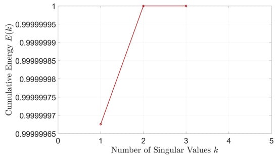
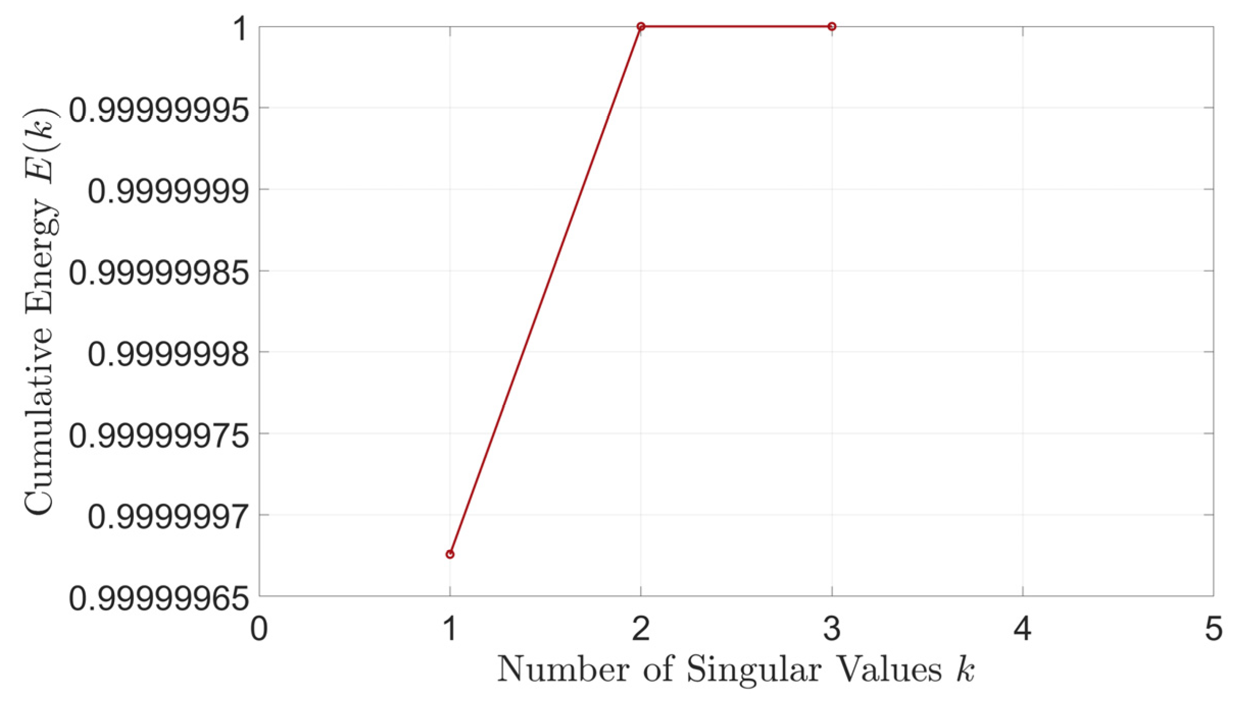
Since the model (23) is a one-dimensional system, the embedding dimension should be at least 3. We initially set the embedding dimension $m=3$ to observe the singular values (Sigs) and plot the variation of $E\left(k\right)$ with $k$, as shown in Figure 1.

$$Sigs=\left[1.8\times {10}^4,1.2,1.1\times {10}^{-3}\right].$$

(24)

Figure 1. Plot of cumulative energy variation with the number of singular values when the parameter set is taken as Para1, m = 3, r = 2.

According to model (24) and Figure 1, when $r=2$, $E\left(k\right)$ can exceed 99% and approach the convergence value. Choosing $r=2$ implies that in this example, we can only plot the two-dimensional embedded flow field and the one-dimensional reconstructed flow field (since with $r=2$, the output matrix of the forced linear model consists of only one column vector).

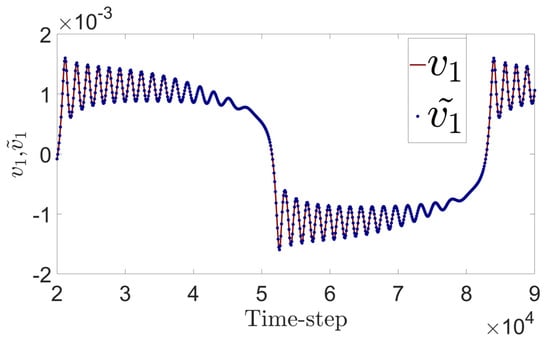
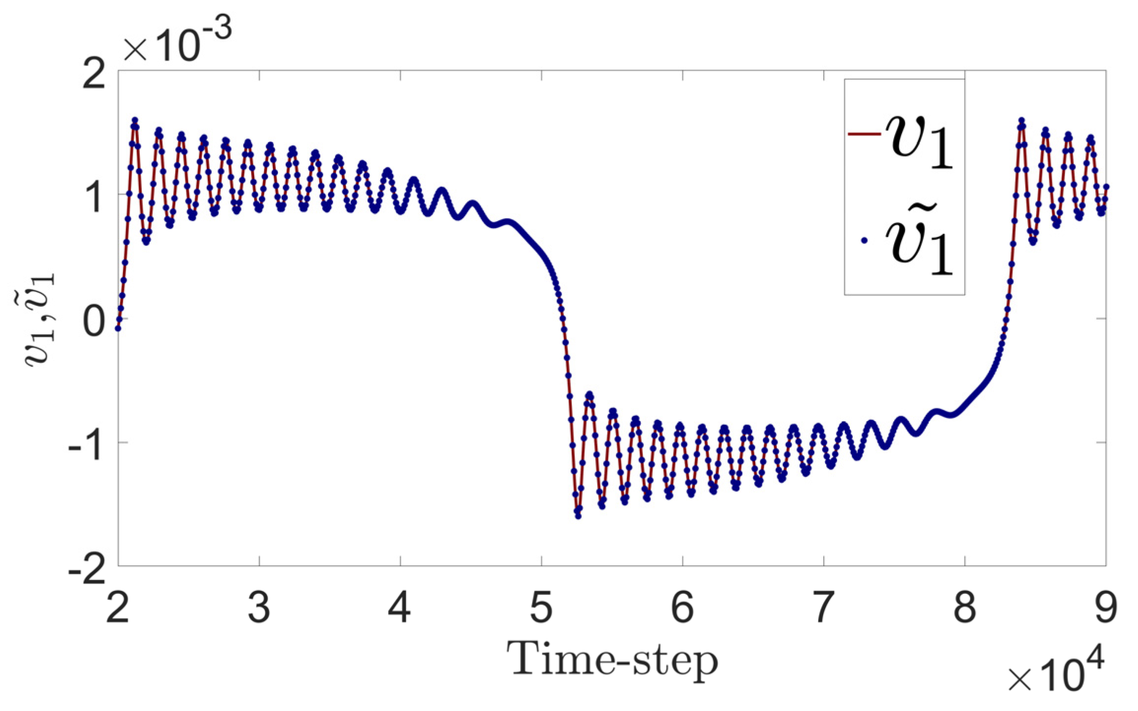
By plotting the fit between the first column of the output matrix and the first column of the input matrix (Figure 2), we can observe the reconstruction performance of the forced linear model. Additionally, the mean squared error (MSE) of the reconstruction at this point is 1.3751 × 10⁻¹⁷.

Figure 2. The output matrix of the forced linear model when the parameter set is Para1, m = 3, r = 2 is plotted against a fit to the first column of the output matrix, where only uniformly spaced (100 ∆t) discrete trajectory points are retained in the first column of the output matrix, labeled as blue points to avoid an overly dense and complex image.

Alternatively model (23) can be rewritten as

$$\left\{\begin{array}{l}\dot{x}=y\\ \dot{y}=-a_2{x}^3-a_{1}x-a_3{y}^3-\alpha x^{4}y-\beta x^{2}y-\lambda y+f_1\cos \left({\omega }_{1}t\right),\end{array}\right.$$

(25)

This treatment allows the researcher to plot the 2D phase diagram (Figure 3b). This allows us to comparatively examine the reconstruction of the 2D-embedded flow field in the 2D time-lag embedding space.

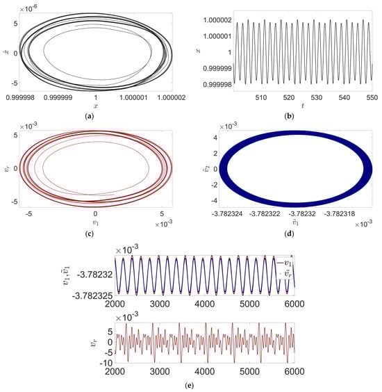
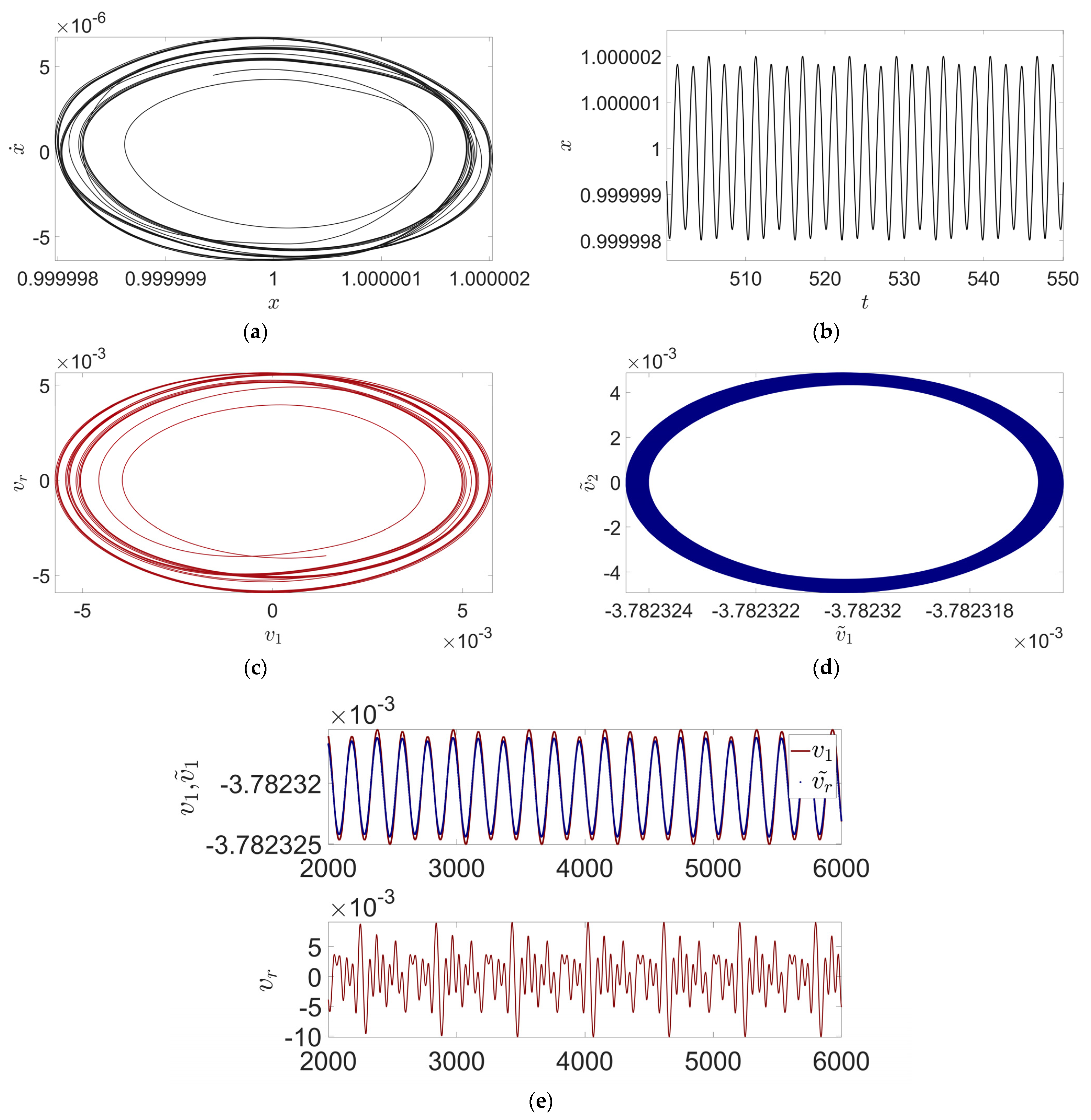
Figure 3. Series of experimental plots when the parameter set is taken to be Para1, m = 3, r = 2. (a) 2D-embedded flow field; (b) Original 2D phase diagram; (c) Upper subplot for the eigentime series $v_1$ and lower subplot for the forced eigentime series $v_r$; (d) Localized enlargement of (c).

Comparing Figure 3a with Figure 3b reveals that the trajectory structures in both images exhibit similar vortex shapes and singularity locations, although the axes and scaling of the images are slightly different (this is due to the fact that Figure 3a is plotted based on the time-step data while Figure 3b is plotted based on the raw time data, hence there is a three-order-of-magnitude difference between the two), the embedded flow field’s overall correspondence between the trajectory morphology and the phase diagram is evident, implying that the embedded flow field performs well in preserving the global topology. A closer look at the local vortex structure and trajectory spacing, the dense length of the trajectories, and the trend of morphology change shows that the embedded flow field is also more successful in restoring the local features. In addition, the trajectories in the embedded flow field retain a similar smoothness to the original phase diagram, with no obvious discrete points or anomalous jumps, which implies that the flow field is also more accurately restored in terms of continuity and smoothness. Thus, assessed visually, the two maps are almost topologically equivalent.

Observe the second subfigure of Figure 3f, where the intermittent periodic bursts observed in the time series $v_r$ of the stressing features indicate that the model (23) under the parameter group Para1 would exhibit bursting oscillatory behavior.

If we take $r=3$ while keeping the embedding dimension $m=3$ constant, then $E\left(k\right)$ still satisfies the condition of being greater than 99%. Although the MSE in this case increases slightly to 1.0795 × ${10}^{-15}$, it is still at a relatively high level. Since we have raised the value of r to 3, we can plot the reconstructed 2D flow field (Figure 4b). As can be seen from the figure, the original 2D phase diagram of the reconstructed 2D flow field as well as the 2D-embedded flow field are likewise almost equivalent in terms of topology.

Figure 4. Series of experimental plots when the parameter set is taken to be Para1, m = 3, r = 3. (a,b) 2D−embedded flow field and its reconstructed flow field; (c) Original 2D phase diagram; (d) 3D-embedded flow field; (e) Reconstructed fitted diagrams, similar to Figure 2; (f) Dominant feature time series vs. forced feature time series.

However, observing Figure 4d we can find that when $m=3, r=3$, the construction of the 3D-embedded flow field fails to maintain the smoothness although we achieve a more accurate and effective 1D and 2D reconstruction (Figure 4e) and capture the emergence of the bursting oscillations by the forced eigenmodes.

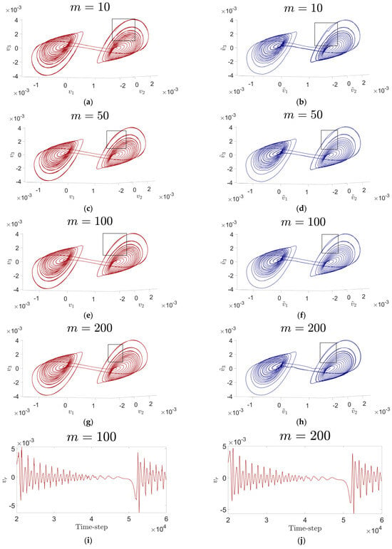
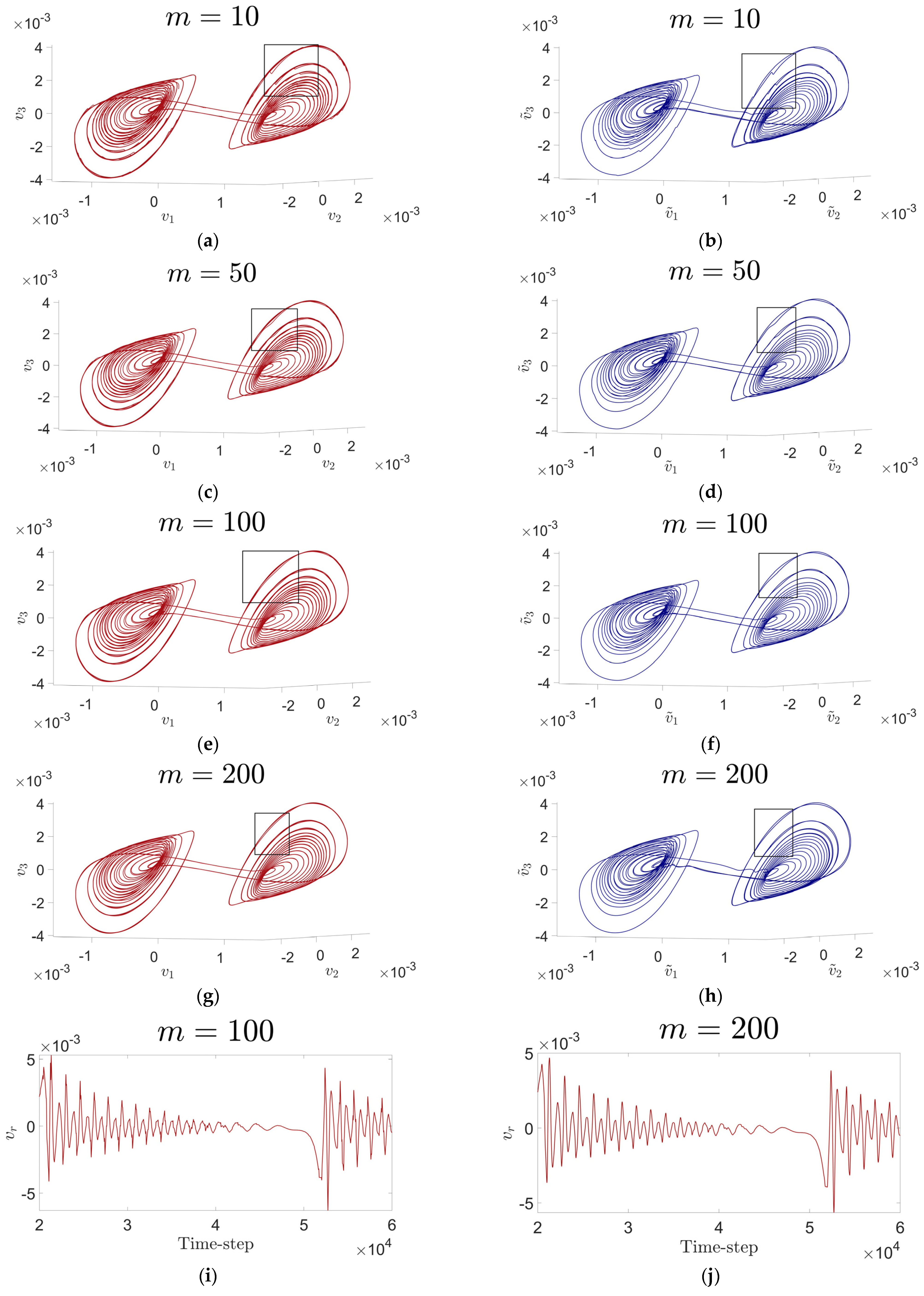
Therefore, we consider fixing $r=4$ (to facilitate the reconstruction of the 3D-embedded flow field), and raising the embedding dimension. Fixing $r=4$ in Figure 5, we record the 3D-embedded flow field plotted when the embedding dimension m takes different values and its reconstructed flow field.

Figure 5. (a–h) Show the two-dimensional-embedded flow field and its two-dimensional reconstructed flow field obtained by taking para1, r = 4, and varying the value of m for model (24). (a,b) $m=10$; (c,d) $m=50$; (e,f) $m=100$; (g,h) $m=200$; (i) Time series of forced features at $m=100$. (j) Time series of stress characteristics at $m=200$. (j) Significantly smoother compared to (i).

Based on Figure 5 and the reconstruction error MSE for each dimension, we organize and obtain Table 1.

Table 1. MSE and Smoothness Metrics for Various Embedding Dimensions.

Embedding Dimension m (r = 4)	MSE	Degree of Smoothness (Embedded Flow Field)	Degree of Smoothing (Time Series of Forced Characteristics)
m = 10	4.8309 × 10−10	low	low
m = 50	2.4387 × 10−11	medium	low
m = 100	2.661 × 10−11	high	medium
m = 200	1.978 × 10−10	high	high

From Table 1 we find that when fixing $r=4$ and increasing the embedding dimension, the MSE has been kept at a relatively low level, which ensures that all our reconstructions have a very low error. However, the performance of different embedding dimensions varies in terms of how smooth the reconstructed flow field is with respect to the time series of the forced features. The embedding dimension $m=200$ is reasonable in terms of reconstruction accuracy and reconstruction smoothness table. However, m = 200 is not necessarily the best choice, and we believe that the choice of the embedding dimension is a problem that needs to be further investigated in the future.

4.2. Advantages

In this section, we demonstrate the advantages of applying HAVOK analysis to the field of bursting oscillations through several comparative experiments. These advantages include: I. Capturing the somewhat hidden bursting oscillations in the time-course profile. II. Embedding the flow field in a higher-dimensional delay space to capture more dynamical features of the original dynamical system, avoiding “overlapping phenomena”, allowing the trajectories to unfold in time-lagged embedded space as well as reconstructed space.

4.2.1. Revealing Hidden Dynamical Behaviors

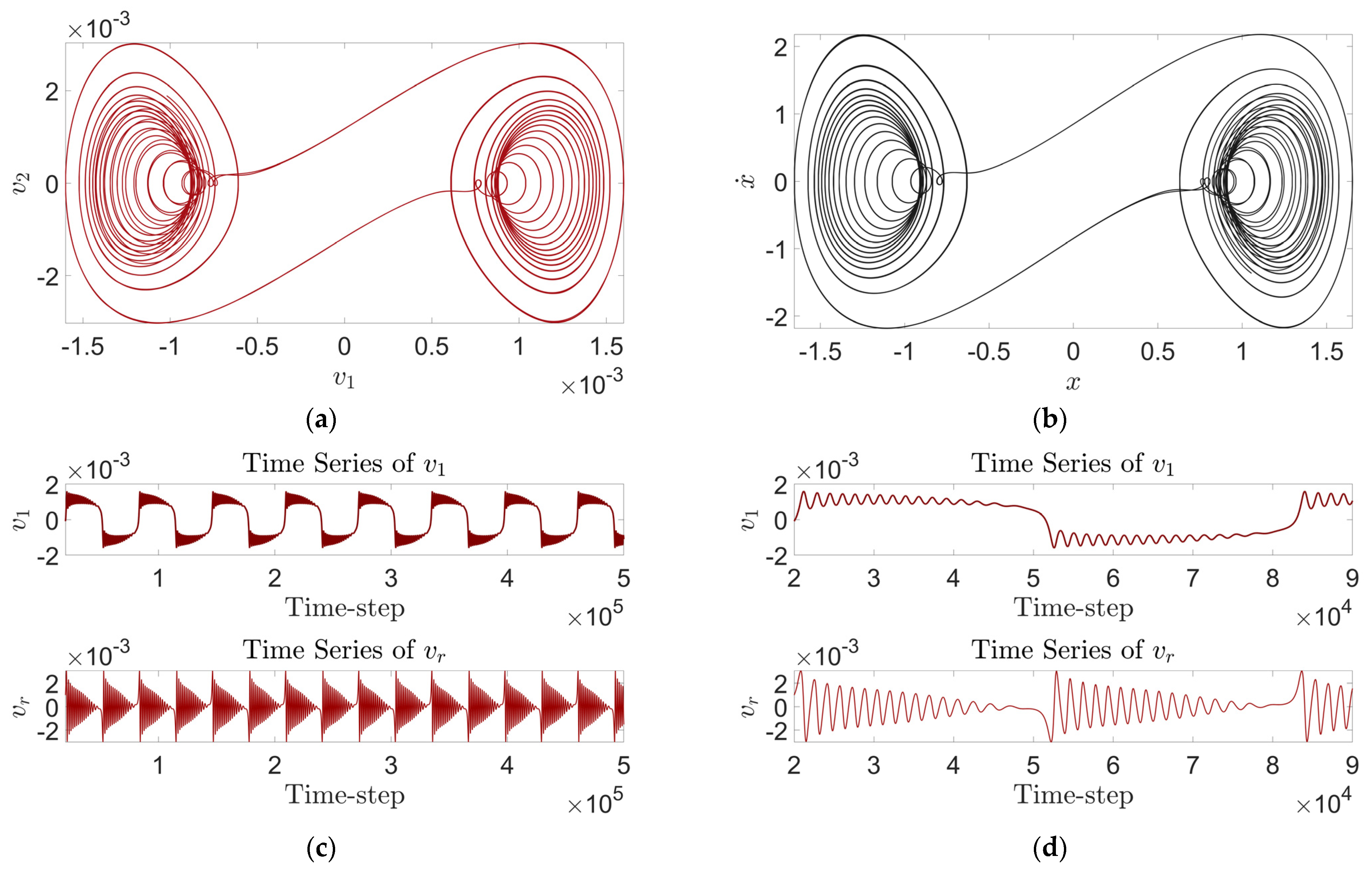
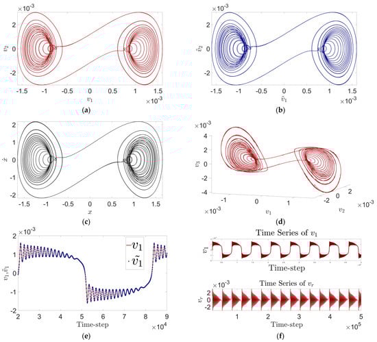
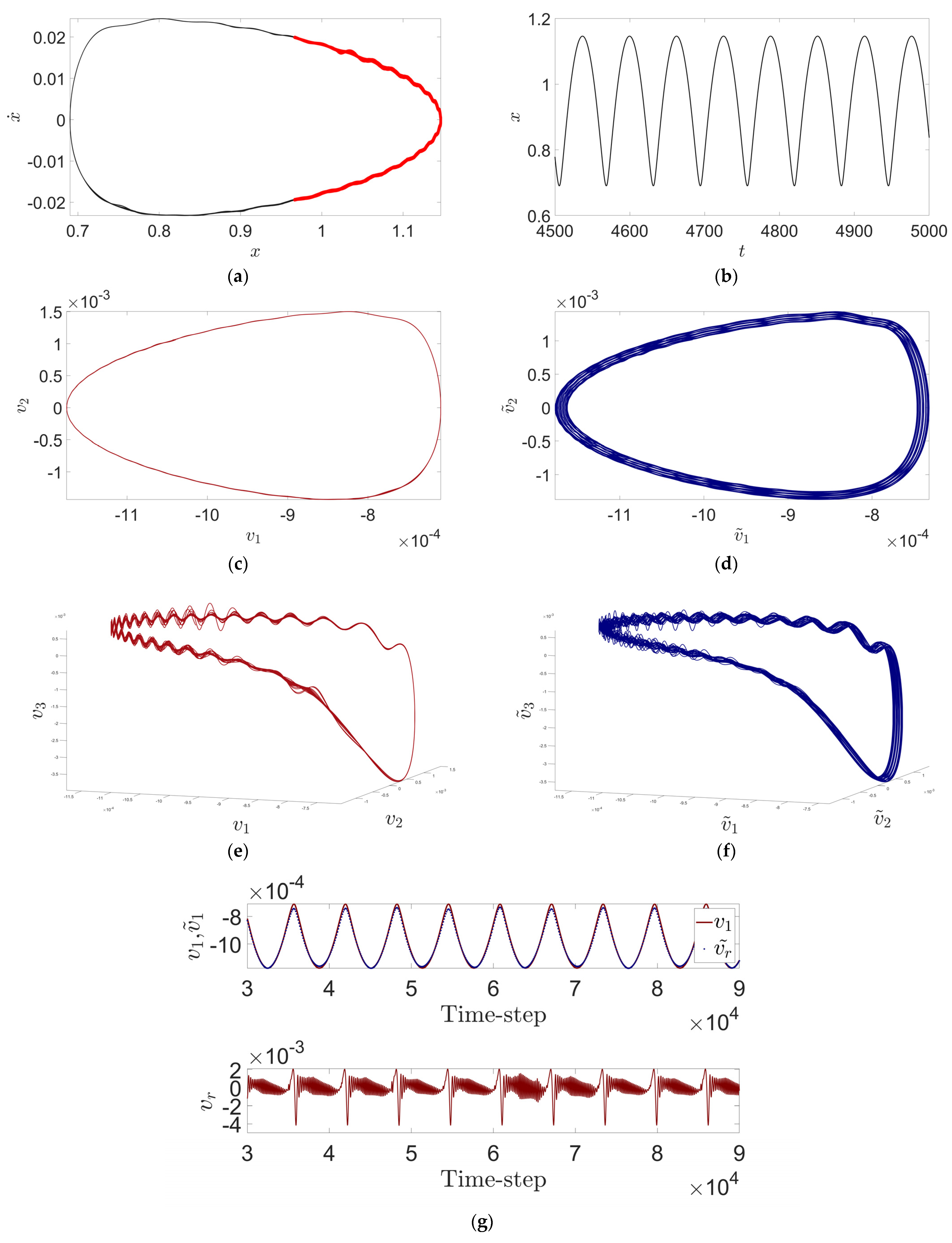
When the parameter set of model (24) is Para2 = $(a_1,a_2,a_3,\alpha ,\beta ,\lambda ,\omega ,f_1)=(-5,5,0.1,0.1,-1,1.2,0.1,1.8)$, the emergence of bursting oscillations is difficult to observe from the time-history curves (Figure 6b), but a slight oscillatory behavior is indeed observed in the two-dimensional phase diagrams (Figure 6a). Using traditional numerical methods, the researcher may have difficulty in relating the behavior between the 1D time-history curve and the 2D phase diagram.

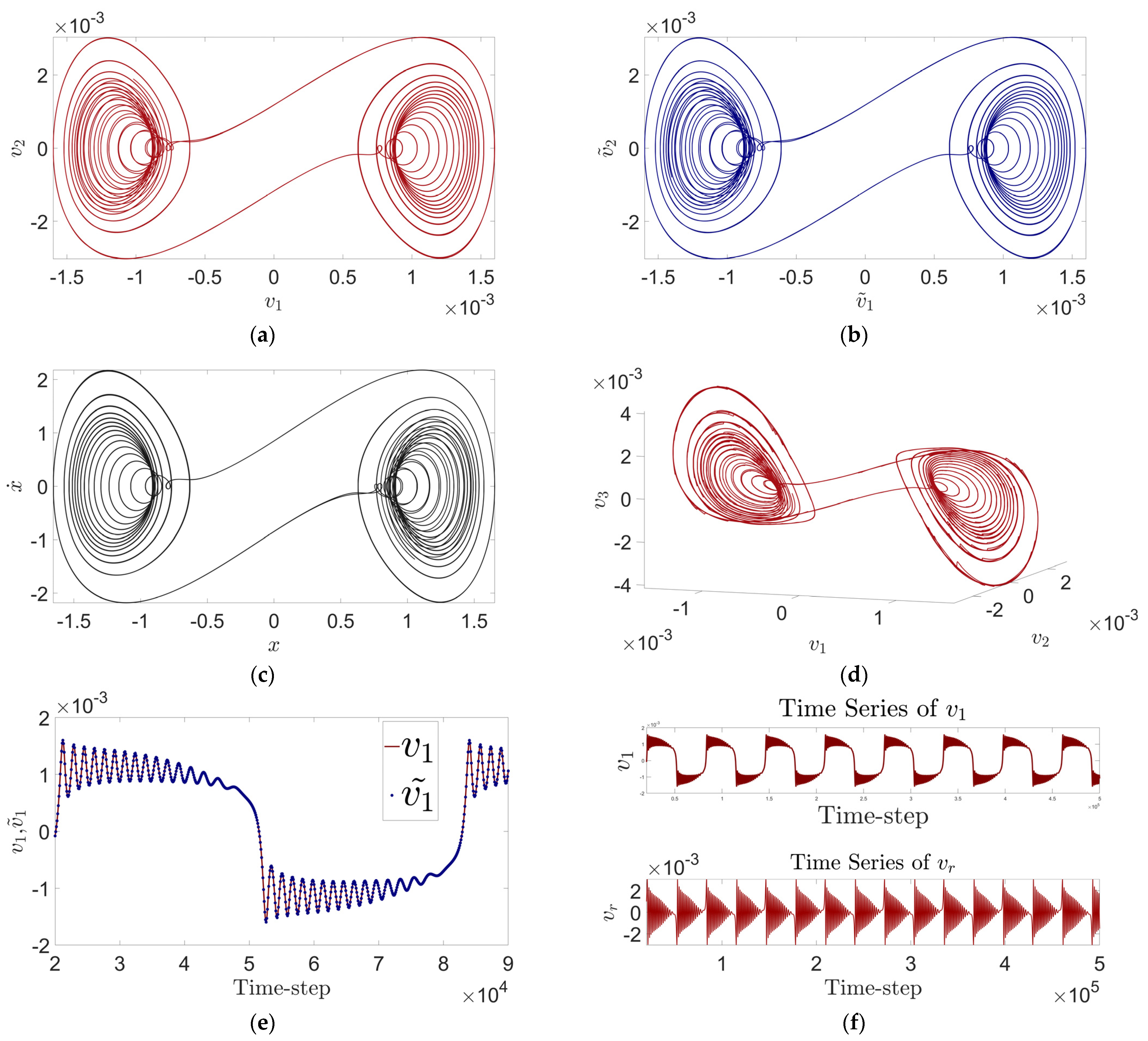
Figure 6. A series of experimental plots taken for the parameter set Para2$, m=200, r=4$. (a) Raw 2D phase diagrams, with the approximate regions where small amplitude oscillations occur marked in red; (b) Time-course curves; (c,e) 2D- and 3D-embedded flow fields; (d,f) Reconstructed 2D and 3D flow fields; (g) Fitted curves to test the effectiveness of the reconstruction in the upper half of the subplot, and time series of the forced features in the lower half of the subplot.

Therefore, we would like to embed the flow field into a higher dimensional time-lag embedded space through time-lag embedding, so as to observe a more comprehensive dynamical behavior of the system. Based on the need to construct a smooth 3D-embedded flow field, we continue the choice of $m=200, r=4$ in Section 4.1. At this time, the MSE = 2.1817e−10. (If the experimental performance is not good or the reconstruction accuracy is too low, the value of $m$ or $r$ can be adjusted according to the experimental feedback).

The periodic intermittent bursting behavior on the time series of the forced features (Figure 6g) captures the phenomenon of hidden bursting oscillations in the time-course profile. The construction of a three-dimensional embedded flow field and its reconstructed flow field demonstrates richer dynamical features of the dynamical system (23) with the parameter Para2. For example, the alternation of low-frequency large-period oscillations and high-frequency small-period oscillations is more obvious in Figure 6g,f, which helps the researcher to understand the oscillatory behaviors of the red part of the two-dimensional phase diagrams, as well as to prevent the researcher from misjudging whether or not bursting oscillatory phenomena occur by observing the one-dimensional time-history curve directly, and thinking that bursting oscillatory phenomena occur or not. and avoiding the researcher from misjudging whether the bursting oscillation phenomenon occurs or not by directly observing the 1D time-history curve and thinking that the bursting oscillation phenomenon does not occur.

In addition, this example also demonstrates the advantage of constructing a three-dimensional embedded flow field over constructing only a two-dimensional embedded flow field, and therefore, in choosing $r$, we preferred to choose $r=4$ for the initial observation.

4.2.2. Reducing Overlapping Phenomena through Higher-Dimensional Embedding

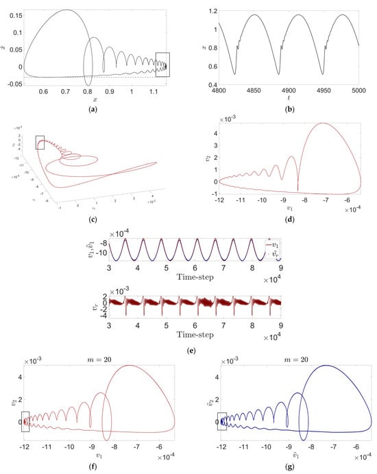
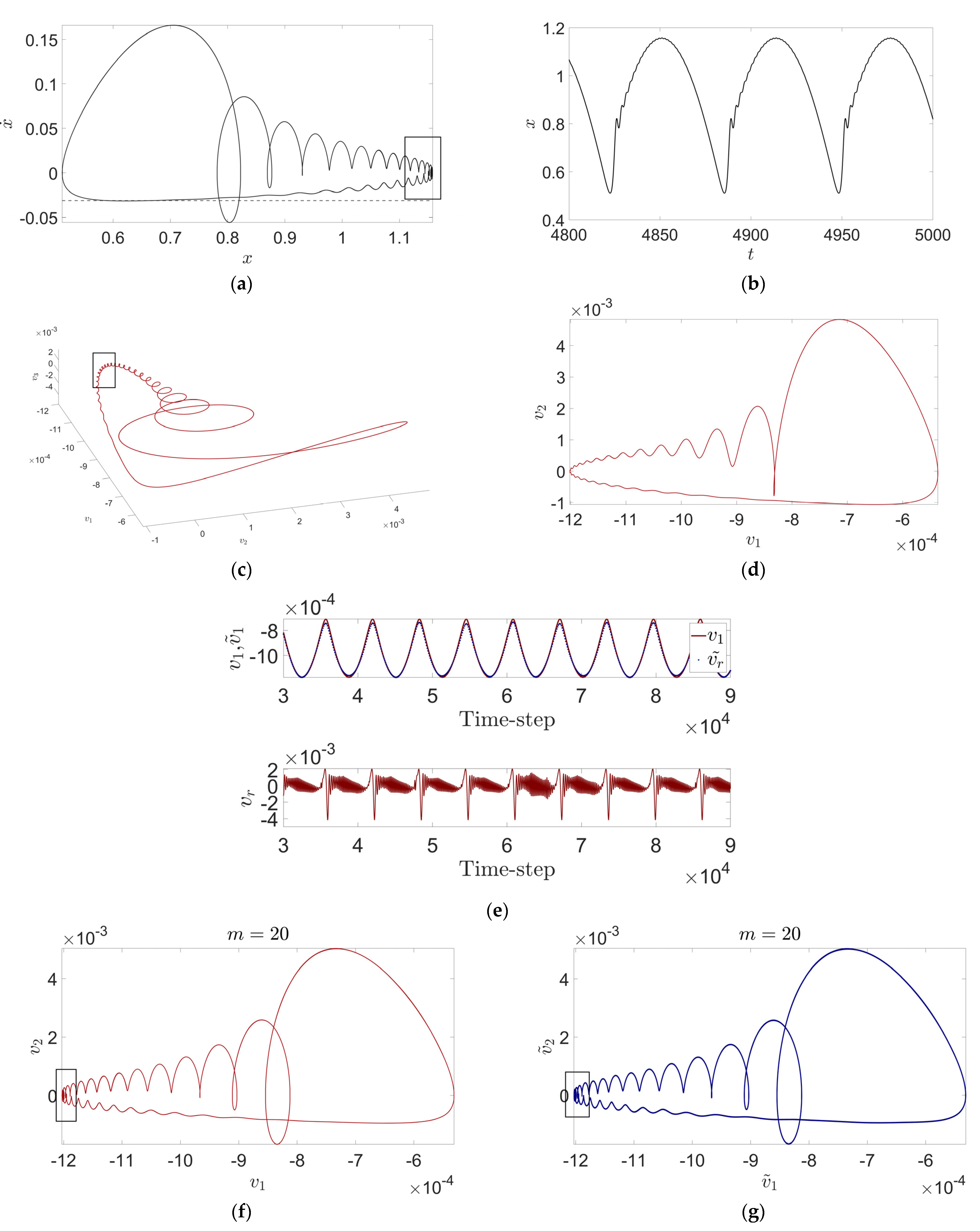
When model (24) is set up with the parameter set Para3 = $({\mathit{a}}_1,{\mathit{a}}_2,{\mathit{a}}_3,\mathit{\alpha },\mathit{\beta },\mathit{\lambda },\mathit{\omega },{\mathit{f}}_{\mathbf{1}})=(-\mathbf{5},\mathbf{5},\mathbf{0.1},\mathbf{0.1}-\mathbf{1},\mathbf{1.2},\mathbf{0.1},\mathbf{1.95}).$ At this point ${\mathit{f}}_{\mathbf{1}}$ is slightly increased compared to the value of ${\mathit{f}}_{\mathbf{1}}$ taken in Para3. We observe a weak bursting oscillation phenomenon in the local zoomed-in plot of the time-course curve (Figure 7), which partly verifies the judgment in Section 4.2.1 about the appearance of bursting oscillation.

Figure 7. (a–e) Show experimental plots with Parameter Set Para3, $r=4$, $m=200$. (a) The original two-dimensional phase diagram, with a box indicating the approximate region where the ‘overlap phenomenon’ occurs; (b) The original time history curve; (c) The three-dimensional-embedded flow field, with a box indicating the approximate region of the ‘overlap phenomenon’ in (a); (d) The two-dimensional-embedded flow field, where the ‘overlap phenomenon’ in the boxed area of (a) disappears; (f,g) are the two-dimensional-embedded flow field and its reconstructed flow field plotted with Parameter Set Para3, $r=4, m=20$, both of which show the same ‘overlap phenomenon’ as in (a).

In addition, the “overlapping phenomenon” in the 2D phase diagram (Figure 7a), where the trajectories overlap in the phase diagram, may lead to the inability of the researcher to correctly distinguish the different states of the system. Embedding the flow field in a higher-dimensional embedded flow field may help to understand the reason for the overlapping phenomenon in the 2D phase diagram. Similarly, based on the need of plotting the 3D-embedded flow, we continue to choose $m=200, r=4.$ At this time, MSE = 3.5956 × ${10}^{-10}$. The reconstruction can be roughly judged to perform well by Figure 7e.

Figure 7c,d and Figure 7f,g show the two-dimensional embedded flow field and its reconstructed flow field at $m=200$ and $m=20$, respectively. By comparing them, we can find that elevating the embedding dimension can make the trajectories more stretched in the embedding space, which may reduce or avoid the reasons for the occurrence of overlapping. This is also one of the reasons why we choose a higher embedding dimension, in the case that the test accuracy meets the experimenter’s needs, choosing a slightly higher embedding dimension is both more able to enhance the smoothness of the mapping in the phase space, and may reduce the overlapping of the mapping in the phase space, which is convenient for analyzing and understanding the dynamical behavior of the system.

4.2.3. Analyzing Quasi-Periodic Behavior and Steady-State Nonlinear Oscillations

In the above example, we primarily focus on situations that may lead to bursting oscillations. However, in some dynamical systems, if certain parameters do not cross a specific threshold, the system may not exhibit bursting oscillations. For instance, setting ${\mathit{f}}_{\mathbf{1}}=0$ in Para1, meaning that for Parameter Set Para4 in model (23), Para4 = $(a_1,a_2,a_3,\alpha ,\beta ,\lambda ,\omega ,{\mathrm{f}}_1)=(-5,5,0.1,0.1-1,1.2,0.1,0).$

According to Figure 8a,b, the system exhibits quasi-periodic behavior. In Figure 8e, more pronounced quasi-periodic behavior can be observed from the forced characteristic time series, but there are no intermittent bursts. Therefore, we conclude that with Parameter Set Para4, system (23) exhibits quasi-periodic behavior but does not display bursting oscillations.

Figure 8. A series of experimental plots taking the parameters Para4,$m=100, r=4.$(a,b) Original 2D phase diagrams with time-course curves; (c,d) 2D-embedded flow field and its reconstructed flow field; (e) Upper subplot shows the fitted curves to test the effect of the reconstruction, and the lower subplot shows the time series of the forced features.

HAVOK analysis is usually used to analyze systems with significant time-varying properties [19], so its application to unsteady systems has been more studied and verified. While there are less studies about its application in the field of steady state nonlinear oscillations. Steady-state nonlinear oscillation refers to a stable oscillatory state that the system enters after a long period of evolution, with little change in amplitude and frequency, although the oscillation itself may be complex, multifrequency or nonperiodic. However, steady-state nonlinear oscillations may also involve complex nonlinear interactions and multiple time scales. Unlike unsteady-state behavior, their dynamic properties are more stable and complex. This example shows to some extent the potential of the HAVOK method for applications in the field of steady-state nonlinear oscillations.

5. Conclusions

In fields such as engineering and neuroscience, the study of bursting oscillations caused by multi-time-scale phenomena has traditionally relied on phase diagrams and time series plots for numerical validation. However, these methods alone may have limitations in accurately detecting bursting oscillations. For example, the phenomenon of bursting oscillations in time series plots may be too subtle, and the “overlap phenomenon” in phase diagrams may complicate the researcher’s understanding of complex phenomena. In this paper, we adopt the HAVOK analysis framework, and in Section 4, we demonstrate through comparative experiments how HAVOK analysis can capture the occurrence of bursting oscillations when they are too subtle to detect through intermittent bursting phenomena in the forced modes. Additionally, we show how the three-dimensional embedding flow field constructed using the time-delay embedding method can provide more dynamic information about the system, highlighting the potential of this method to address the “overlap phenomenon” that may occur in phase diagrams. These advantages over traditional numerical simulation methods may facilitate a more comprehensive understanding of the system’s dynamic characteristics by researchers.

Due to current technical limitations, we have not rigorously determined the optimal embedding dimension $m$ and truncation order $r$ in this paper, and we have found that these two factors can have some impact on the experimental results. This will be a direction for our future research.

References

- Fang, Z.W.; Zhang, Y.W.; Li, X.; Ding, H.; Chen, L.Q. Integration of a nonlinear energy sink and a giant magnetostrictive energy harvester. J. Sound Vib. 2017, 391, 35–49. [Google Scholar] [CrossRef]
- Zhang, Y.W.; Lu, Y.N.; Chen, L.Q. Energy harvesting via nonlinear energy sink for whole spacecraft. Sci. China Technol. Sci. 2019, 62, 1483–1491. [Google Scholar] [CrossRef]
- Yang, T.Z.; Hou, S.A.; Qin, Z.H.; Ding, Q.; Chen, L.Q. A dynamic reconfigurable nonlinear energy sink. J. Sound Vib. 2020, 493, 115629. [Google Scholar] [CrossRef]
- Zang, J.; Cao, R.Q.; Zhang, Y.W.; Fang, B.; Chen, L.Q. A lever-enhanced nonlinear energy sink absorber harvesting vibratory energy via giant magnetostrictive-piezoelectricity. Commun. Nonlinear Sci. Numer. Simul. 2021, 95, 105620. [Google Scholar] [CrossRef]
- Zhang, W.; Liu, Y.Z.; Wu, M.Q. Theory and experiment of nonlinear vibrations and dynamic snap-through phenomena for bi-stable asymmetric laminated composite square panels under foundation excitation. Compos. Struct. 2019, 225, 111140. [Google Scholar] [CrossRef]
- Karami, H.; Karimi, S.; Bonakdari, H.; Shamshirband, S. Predicting discharge coefficient of triangular labyrinth weir using extreme learning machine, artificial neural network and genetic programming. Neural Comput. Appl. 2018, 29, 983–989. [Google Scholar] [CrossRef]
- Kumar, P.; Kumar, A.; Erlicher, S. A modified hybrid Van der Pol-Duffing-Rayleigh oscillator for modelling the lateral walking force on a rigid floor. Phys. D Nonlinear Phenom. 2017, 358, 1–14. [Google Scholar] [CrossRef]
- Kuehn, C. Multiple Time Scale Dynamics; Springer: Berlin/Heidelberg, Germany, 2015. [Google Scholar] [CrossRef]
- Qian, Y.H.; Wang, H.L.; Zhang, D.J. Bursting Dynamics in the General Hybrid Rayleigh-van der Pol-Duffing Oscillator with Two External Periodic Excitations. J. Vib. Eng. Technol. 2023, 12, 2943–2957. [Google Scholar] [CrossRef]
- Ma, X.D.; Bi, Q.S.; Wang, L.F. Complex bursting dynamics in the cubic-quintic Duffing-van der Pol system with two external periodic excitations. Meccanica 2022, 57, 1747–1766. [Google Scholar] [CrossRef]
- Rinzel, J. Bursting oscillations in an excitable membrane model. Ordinary Part. Differ. Equ. 1985, 1151, 304–316. [Google Scholar]
- Brunton, S.L.; Brunton, B.W.; Proctor, J.L.; Kutz, J.N. Koopman invariant subspaces and finite linear representations of nonlinear dynamical systems for control. PLoS ONE 2016, 11, e0150171. [Google Scholar] [CrossRef] [PubMed]
- Budišić, M.; Mohr, R.M.; Mezić, I. Applied koopmanism. Chaos 2012, 22, 047510. [Google Scholar] [CrossRef]
- Jin, Y.H.; Hou, L.; Zhong, S.; Yi, H.M.; Chen, Y.S. Invertible Koopman Network and its application in data-driven modeling for dynamic systems. Mech. Syst. Signal Process. 2023, 200, 110604. [Google Scholar] [CrossRef]
- Takens, F. Detecting strange attractors in turbulence. In Dynamical Systems and Turbulence. Warwick, Lecture Notes in Mathematics; Rand, D., Young, L.-S., Eds.; Springer: Berlin/Heidelberg, Germany, 1981; pp. 366–381. [Google Scholar] [CrossRef]
- Tu, J.H.; Rowley, C.W.; Luchtenburg, D.M.; Brunton, S.L.; Kutz, J.N. On dynamic mode decomposition: Theory and applications. J. Comput. Dyn. 2014, 1, 391–421. [Google Scholar] [CrossRef]
- Arbabi, H.; Mezić, I. Ergodic theory, dynamic mode decomposition, and computation of spectral properties of the Koopman operator. SIAM J. Appl. Dyn. Syst. 2017, 16, 2096–2126. [Google Scholar] [CrossRef]
- Schmid, P.J. Dynamic Mode Decomposition and Its Variants. Annu. Rev. Fluid Mech. 2022, 54, 225–254. [Google Scholar] [CrossRef]
- Brunton, S.L.; Brunton, B.W.; Proctor, J.L.; Kaiser, E.; Kutz, J.N. Chaos as an intermittently forced linear system. Nat. Commun. 2017, 8, 19. [Google Scholar] [CrossRef] [PubMed]
- Brunton, B.W.; Johnson, L.A.; Ojemann, J.G.; Kutz, J.N. Extracting spatial–temporal coherent patterns in large-scale neural recordings using dynamic mode decomposition. J. Neurosci. Methods 2016, 258, 1–15. [Google Scholar] [CrossRef] [PubMed]
- Hirsh, S.M.; Ichinaga, S.M.; Brunton, S.L.; Kutz, J.N.; Brunton, B.W. Structured timedelay models for dynamical systems with connections to Frenet-Serret frame. Proc. R. Soc. A 2021, 477, 20210097. [Google Scholar] [CrossRef] [PubMed]
Disclaimer/Publisher’s Note: The statements, opinions and data contained in all publications are solely those of the individual author(s) and contributor(s) and not of MDPI and/or the editor(s). MDPI and/or the editor(s) disclaim responsibility for any injury to people or property resulting from any ideas, methods, instructions or products referred to in the content. |
© 2024 by the authors. Licensee MDPI, Basel, Switzerland. This article is an open access article distributed under the terms and conditions of the Creative Commons Attribution (CC BY) license (https://creativecommons.org/licenses/by/4.0/).