Numerical Algorithms for Identification of Convection Coefficient and Source in a Magnetohydrodynamics Flow

Abstract

We consider three integral observations inverse problems (IP1, IP2, IP3) for reconstruction of a time-dependent convection coefficient and a source in magnetohydrodynamics (MHD) model. On the first stage, using the integral observations, we reduce the inverse problems to nonclassical direct (forward) ones. The equivalence between the inverse and direct problems is established. Then, the well-posedness of nonclassical problems is proved. Further, to overcome the difficulties arising from the nonlinear nonlocal parabolic operators, we construct a linarization algorithm in time after their difference space discretizatons. Next, on each iteration, to solve the corresponding linear systems of algebraic equations, we propose adequate fast elimination algorithms. Computational results of test examples data are discussed.

1. Introduction

The research concerning the construction and analysis of numerical methods for partial differential equations (PDEs) is more developed and actual than analytical methods. It is due to the necessity of solving many problems of physics, mechanics, heat-mass transfer, finance, biology, etc., see e.g., [1,2,3,4,5,6,7,8], for which it is difficult to construct analytical solutions. The main interest in efficient numerical solving of the PDEs in applied science and engineering is concerned with construction of fast computational algorithms.

The inverse problem is formulated for a particular process described by a PDE when one or some important data such as a coefficients, boundary data, and source data, are provided in many publications [1,9,10,11,12,13,14,15,16,17,18,19,20,21]. In the current paper, we study a convection coefficient and a source inverse problem of a parabolic system from MHD.

In recent years, the viscous MHD duct flows, as a challenging and problem arising in the fields of physics and engineering, have considerable theoretical and practical importance owing to their important and widespread applications in astrophysics, geology, designing cooling systems with liquid metals for a nuclear fission or fusion reactor, power generation, MHD generators, and electromagnetic pumps. A number of theoretical and experimental studies have been performed for the aforementioned.

Because of the coupling of the equations of fluid mechanics and electrodynamics, the solution of the equations governing MHD flows is quite difficult, so analytical solutions are available only in some special cases. For this reason, in the general situation, the MHD flow problems can be only numerically solved by taking advantage of some numerical methods [4,15].

While steady MHD duct flows have been studied extensively, some papers have appeared on unsteady 2D incompressible, viscous MHD flow in channels. Works on time-dependent MHD flow systems, concerning the areas of the flow control and the MHD stability, have investigated different problems. These related control and stability problems for the MHD flows are all model-based approaches, in which the model parameters or the initial conditions have to be identified. However, when model parameters (i.e., empirical parameters and initial conditions) are unknown or uncertain, it often leads to biased simulation results and inconsistencies between the output of the established control system and the real physical system. Thus, it is fundamentally important to recover these various unknown or uncertain parameters in the direct system model so that the mathematical model can best fit the real physical system under considerations. Such problems are commonly referred to as parameter estimation problems or inverse problems in the areas of data assimilation. In the paper, we consider a recovering problem for a simplified MHD Hartman flow with characteristics of incompressible and Newtonian (constant viscosity) in 1-D space. The mathematical model of the 1-D MHD Hartman flow can be successfully built under some suitable assumptions and tightly coupled by the flow velocity and electromagnetic fields [17,21].

Least squares cost functionals are often used for parameter estimation of the objective functions. However, such estimation procedures (gradient-like search) are computationally time-consuming [11,22]. Also, through each step in the iteration, the solutions of forward problems of PDEs have to be solved numerically. In this paper, we propose a direct system method to avoid these drawbacks. This approach leads to the technique of the loaded equation method, first introduced for the solution of the source heat problem in [6].

In [23], a Galerkin finite element method was used for solving an inverse problem, similar to IP1, described in Section 2.2 of the present paper.

This paper is structured as follows. In the next section, the direct and the inverse problems are introduced. Algorithms that transform the inverse problems into nonclassical direct problems are proposed in Section 3. Section 4 develops algorithms for the numerical solution of the direct problem. In Section 5, effective decomposition algorithms for the solution of the difference algebraic systems are constructed. Numerical test examples are discussed in Section 6. This paper is finalized with some conclusions.

2. Formulation of the Direct and Inverse Problems

In this section, the direct (forward) and inverse problems to a strongly coupled system of two parabolic equations of a viscous MHD flow are formulated.

2.1. The Direct Problem

We will study the model considered in [17,24,25]. It is a simplified MHD Hartman flow with incompressible and Newtonian (constant viscosity) characteristics in 1-D space and the case in which the fluid flows between two parallel solid plates and the velocity is perpendicular to the magnetic vector. Also, for the unit vectors of the velocity, the magnetic fields’ external electromotive forces are generated right-handed. This mathematical model of describing the 1-D MHD flow system is derived from the viscous incompressible MHD equations [17,21,24] and is formulated in the following form:

$$\begin{array}{ccc}\hfill {\displaystyle \frac{\partial u}{\partial t}}-\nu {\displaystyle \frac{{\partial }^{2}u}{\partial x^2}}& =& \beta \left(t\right){\displaystyle \frac{\partial B}{\partial x}}-f\left(t\right),\hfill \end{array}$$

(1)

$$\begin{array}{ccc}\hfill {\displaystyle \frac{\partial B}{\partial t}}-{\nu }_m{\displaystyle \frac{{\partial }^{2}B}{\partial x^2}}& =& \beta \left(t\right){\displaystyle \frac{\partial u}{\partial x}}.\hfill \end{array}$$

(2)

Here, the spatial variable x and the time variable t belong to the set $(x,t)\in Q_T=\Omega \times (0,T),\Omega =(0,X)$, where X and T are dimensionless quantities, $u(x,t)$ is the flow velocity, and $B(x,t)$ is the magnetic field. Further, $f\left(t\right)$ is the pressure difference per unit of the channel length; the function $\beta \left(t\right)$ is a given function of the induction of the external magnetic field and can be considered as the control input for the MHD flow; $\nu =1/Re$ and ${\nu }_m=1/R{e}_m$, where $Re$ is the flow Reynolds number and $R{e}_m$ is the magnetic Reynolds number.

Dirichlet boundary conditions for the system (1) and (2) are posed:

$$u(0,t)=u_l\left(t\right),u(X,t)=u_r\left(t\right),B(0,t)=B_l\left(t\right),B(X,t)=B_r\left(t\right)$$

(3)

and the initial conditions are

$$u(x,0)=u_0\left(x\right),B(x,0)=B_0\left(x\right).$$

(4)

In the form (1)–(4), we solve the direct (forward) problem in which $f\left(t\right)$, the coefficients $\nu ,{\nu }_m,\beta \left(t\right)$, the boundary, and the initial conditions are given.

2.2. The Inverse Problems

Consider the inverse problem (IP1), in which, simultaneously, the coefficient $\beta \left(t\right)$ and the source term $f\left(t\right)$ are unknowns and will be reconstructed upon the additional conditions

$${\int }_{\Omega }u(x,t){\eta }_1\left(x\right)dx=\phi \left(t\right),{\int }_{\Omega }B(x,t){\eta }_2\left(x\right)dx=\psi \left(t\right),$$

(5)

where ${\eta }_1\left(x\right)$ and ${\eta }_2\left(x\right)$ are some weight functions. In particular, if some of the weight functions are Dirac-Delta functions

$${\eta }_1\left(x\right)=\delta (x-x_{\ast }),{\eta }_2\left(x\right)=\delta (x-x^{\ast }),(x_{\ast },x^{\ast })\in \Omega ,$$

then the conditions (5) take the form

$$u(x_{\ast },t)=\phi \left(t\right),B(x^{\ast },t)=\psi \left(t\right).$$

(6)

In this work, we use ${\eta }_1\left(x\right)={\eta }_2\left(x\right)=1$ and then the total energy takes the simple form

$$\begin{array}{ccc}\hfill {\int }_0^{X}u(x,t)dx& =& E\left(t\right),\hfill \end{array}$$

(7)

$$\begin{array}{ccc}\hfill {\int }_0^{X}B(x,t)dx& =& F\left(t\right).\hfill \end{array}$$

(8)

Here, $E\left(t\right)$ and $F\left(t\right)$ are known functions.

We also will study the following inverse problems:

IP2. The convection coefficient $\beta \left(t\right)$ is known, but the source $f\left(t\right)$ is unknown and the overdetermination (7) is given.

IP3. The convection coefficient $\beta \left(t\right)$ is unknown, but the source $f\left(t\right)$ is known and the overdetermination (8) is given.

Least squares is often used to define the closeness between the computed solutions and the solution measured data objective functional. The resulting methods are referred to as least squares output error criteria procedures; see, e.g., [1,3,6]. Such procedures, along with many advantages, also have their disadvantages. For example, they are computationally consuming because iterative procedures (gradient-like search) are used. In addition, through each step in the iteration, they will reduce to the solution of some forward problem which involves the numerical solution of partial differential equations. Thus, there is a clear need to minimize the number of steps in the iteration as well as reduce the range of the global search. One way this can be achieved is to obtain an independent initial estimate of the structure of the control parameters.

Our goal here is to construct a direct approach to solve the problems IP1, IP2, and IP3. We transform the time-dependent functions identification problems into a nonclassical forward problem. For this, we use the obvious idea of differentiating the relations (7) and (8) with respect to time t and then to insert the time derivative of the flow velocity u and the magnetic field B into the Equations (1) and (2), respectively. As a result, we obtain a new direct initial boundary value problem for the solution $\{u,B\}$. Then, we concentrate on the construction of efficient finite difference algorithms for solving the nonstandard direct differential problems.

3. Reduction of the IP1, IP2, and IP3 to Nonclassical Problems

In this section, we formulate the three inverse coefficient-source problems.

Let us differentiate $E\left(t\right)$ with respect to t, and using Equation (1) and the first boundary conditions in (3), we find

$$f\left(t\right)=\left(\nu (u_x(X,t)-u_x(0,t))+\beta \left(t\right)h\left(t\right)-E^{\prime }\left(t\right)\right)/X,h\left(t\right)=B_r\left(t\right)-B_l\left(t\right),$$

(9)

where $E^{\prime }={\displaystyle \frac{d}{dt}}E,u_x={\displaystyle \frac{\partial u}{\partial x}}$. Next, we differentiate $F\left(t\right)$ with respect to t, and using Equation (2) and the second boundary conditions in (3), we obtain

$$\beta \left(t\right)=(F^{\prime }\left(t\right)-{\nu }_m(B_x(X,t)-B_x(0,t)))/g\left(t\right),g\left(t\right)=u_r\left(t\right)-u_l\left(t\right),$$

(10)

where $F^{\prime }={\displaystyle \frac{d}{dt}}F$ and $B_x={\displaystyle \frac{\partial B}{\partial x}}$.

Let us introduce new solution functions to obtain zero boundary conditions:

$$\begin{array}{ccc}\hfill U(x,t)& =& u(x,t)-\left((1-{\displaystyle \frac{x}{X}})u_l\left(t\right)+{\displaystyle \frac{x}{X}}{u}_r\left(t\right)\right),\hfill \end{array}$$

(11)

$$\begin{array}{ccc}\hfill b(x,t)& =& B(x,t)-\left((1-{\displaystyle \frac{x}{X}})B_l\left(t\right)+{\displaystyle \frac{x}{X}}{B}_r\left(t\right)\right).\hfill \end{array}$$

(12)

Applying these transformations to the problem (1)–(4), we arrive at the following nonclassical forms of (1)–(4).

IP1. Let us suppose that $\beta \left(t\right)$ and $f\left(t\right)$ are unknowns and the overdeterminations (7), (8) are given. Then the reduced (nonclassical) problem reads as follows:

$$\begin{array}{ccc}\hfill {\displaystyle \frac{\partial U}{\partial t}}& -& \nu {\displaystyle \frac{{\partial }^{2}U}{\partial x^2}}-{\displaystyle \frac{F^{\prime }\left(t\right)-{\nu }_m(b_x(X,t)-b_x(0,t))}{g\left(t\right)}}{\displaystyle \frac{\partial b}{\partial x}}\hfill \\ & =& {\displaystyle \frac{E^{\prime }\left(t\right)}{X}}-{\displaystyle \frac{\nu }{X}}\left(U_x(X,t)-U_x(0,t)\right)-\left((1-{\displaystyle \frac{x}{X}})u_l^{\prime }\left(t\right)+{\displaystyle \frac{x}{X}}{u}_r^{\prime }\left(t\right)\right),\hfill \end{array}$$

(13)

$$\begin{array}{ccc}\hfill {\displaystyle \frac{\partial b}{\partial t}}& -& {\nu }_m{\displaystyle \frac{{\partial }^{2}b}{\partial x^2}}-{\displaystyle \frac{F^{\prime }\left(t\right)-{\nu }_m(b_x(X,t)-b_x(0,t))}{g\left(t\right)}}{\displaystyle \frac{\partial U}{\partial x}}\hfill \\ & =& {\displaystyle \frac{F^{\prime }\left(t\right)}{X}}-{\displaystyle \frac{{\nu }_m}{X}}\left(b_x(X,t)-b_x(0,t)\right)-\left((1-{\displaystyle \frac{x}{X}})B_l^{\prime }\left(t\right)+{\displaystyle \frac{x}{X}}{B}_r^{\prime }\left(t\right)\right)\hfill \end{array}$$

(14)

with new initial conditions

$$\begin{array}{ccc}\hfill U(x,0)& =& u_0\left(x\right)-\left((1-{\displaystyle \frac{x}{X}})u_l\left(0\right)+{\displaystyle \frac{x}{X}}{u}_r\left(0\right)\right)\equiv U_0\left(x\right),\hfill \end{array}$$

(15)

$$\begin{array}{ccc}\hfill b(x,0)& =& B_0\left(x\right)-\left((1-{\displaystyle \frac{x}{X}})B_l\left(0\right)+{\displaystyle \frac{x}{X}}{B}_r\left(0\right)\right)\equiv b_0\left(x\right)\hfill \end{array}$$

(16)

and zero Dirichlet boundary conditions.

IP2. Now, let us suppose that $\beta \left(t\right)$ is a known function, but $f\left(t\right)$ is unknown, and the overdetermination (7) is given. Then the nonclassical problem reads as the following parabolic system:

$$\begin{array}{ccc}\hfill {\displaystyle \frac{\partial U}{\partial t}}& -& \nu {\displaystyle \frac{{\partial }^{2}U}{\partial x^2}}-\beta \left(t\right){\displaystyle \frac{\partial b}{\partial x}}\hfill \\ & =& {\displaystyle \frac{E^{\prime }\left(t\right)}{X}}-{\displaystyle \frac{\nu }{X}}\left(U_x(X,t)-U_x(0,t)\right)-\left((1-{\displaystyle \frac{x}{X}})u_l^{\prime }\left(t\right)+{\displaystyle \frac{x}{X}}{u}_r^{\prime }\left(t\right)\right)-{\displaystyle \frac{\nu }{X^2}}g\left(t\right),\hfill \end{array}$$

(17)

$$\begin{array}{ccc}\hfill {\displaystyle \frac{\partial b}{\partial t}}& -& {\nu }_m{\displaystyle \frac{{\partial }^{2}b}{\partial x^2}}-\beta \left(t\right){\displaystyle \frac{\partial U}{\partial x}}\hfill \\ & =& {\displaystyle \frac{\beta }{X}}g\left(t\right)-\left((1-{\displaystyle \frac{x}{X}})B_l^{\prime }\left(t\right)+{\displaystyle \frac{x}{X}}{B}_r^{\prime }\left(t\right)\right)\hfill \end{array}$$

(18)

with initial conditions (15), (16) and zero Dirichlet boundary conditions.

IP3. Finally, let us suppose that $\beta \left(t\right)$ is an unknown function, but $f\left(t\right)$ is known and the overdetermination (8) is given. Then the reduced problem reads as follows:

$$\begin{array}{ccc}\hfill {\displaystyle \frac{\partial U}{\partial t}}& -& \nu {\displaystyle \frac{{\partial }^{2}U}{\partial x^2}}-{\displaystyle \frac{1}{g\left(t\right)}}(F^{\prime }\left(t\right)-{\nu }_m(b_x(X,t)-b_x(0,t))+{\displaystyle \frac{{\nu }_m}{X}}h\left(t\right)){\displaystyle \frac{\partial b}{\partial x}}\hfill \\ & +& {\displaystyle \frac{{\nu }_{m}h\left(t\right)}{Xg\left(t\right)}}(b_x(X,t)-b_x(0,t))\hfill \\ & =& {\displaystyle \frac{h\left(t\right)}{Xg\left(t\right)}}\left(F^{\prime }\left(t\right)+{\displaystyle \frac{\nu }{X}}h\left(t\right)\right)-f\left(t\right)\hfill \\ & -& \left((1-{\displaystyle \frac{x}{X}})u_l^{\prime }\left(t\right)+{\displaystyle \frac{x}{X}}{u}_r^{\prime }\left(t\right)\right)+\left(F^{\prime }\left(t\right)+{\displaystyle \frac{{\nu }_m}{X}}h\left(t\right)\right){\displaystyle \frac{h\left(t\right)}{Xg\left(t\right)}},\hfill \end{array}$$

(19)

$$\begin{array}{ccc}\hfill {\displaystyle \frac{\partial b}{\partial t}}& -& {\nu }_m{\displaystyle \frac{{\partial }^{2}b}{\partial x^2}}-{\displaystyle \frac{1}{g\left(t\right)}}\left(F^{\prime }\left(t\right)-{\nu }_m(b_x(X,t)-b_x(0,t))+{\displaystyle \frac{{\nu }_m}{X}}h\left(t\right)\right){\displaystyle \frac{\partial U}{\partial x}}\hfill \\ & +& {\displaystyle \frac{{\nu }_{m}h\left(t\right)}{Xg\left(t\right)}}(b_x(X,t)-b_x(0,t))\hfill \\ & =& -\left((1-{\displaystyle \frac{x}{X}})B_l^{\prime }\left(t\right)+{\displaystyle \frac{x}{X}}{B}_r^{\prime }\left(t\right)\right)+\left(F^{\prime }\left(t\right)+{\displaystyle \frac{{\nu }_m}{X}}h\left(t\right)\right){\displaystyle \frac{h\left(t\right)}{Xg\left(t\right)}},\hfill \end{array}$$

(20)

with initial conditions (15), (16) and zero Dirichlet boundary conditions.

In all cases, there appear terms $U_x(0,t)$, $U_x(X,t)$ or $b_x(0,t)$, $b_x(X,t)$ in the differential equations. Such equations are called loaded equations; see, e.g., [6,26].

4. Well-Posedness of the Inverse Problems

In this section, we study the well-posedness, i.e., the existence, uniqueness, and continuous dependence on input data of the solutions to the inverse problems. The strategy is first to establish the equivalence between IP1, IP2, and IP3 and the corresponding NCIBVP. More in detail, we shall investigate the case of IP2.

4.1. The IP2

We reformulate the nonclassical initial-boundary value problem (NCIBVP) (17), (18) in a form more suitable for theoretical theoretical analysis. For this, we rewrite the system (17), (18) as follows:

$${\displaystyle \frac{\partial U}{\partial t}}-\nu {\displaystyle \frac{{\partial }^{2}U}{\partial x^2}}-\beta \left(t\right){\displaystyle \frac{\partial b}{\partial x}}+{\displaystyle \frac{\nu }{X}}(U_x(X,t)-U_x(0,t))=R(x,t),$$

(21)

$${\displaystyle \frac{\partial b}{\partial t}}-{\nu }_m{\displaystyle \frac{{\partial }^{2}b}{\partial x^2}}-\beta \left(t\right){\displaystyle \frac{\partial U}{\partial x}}=S(x,t),$$

(22)

where

$$R(x,t)={\displaystyle \frac{E^{\prime }\left(t\right)}{X}}-u_l^{\prime }\left(t\right)-{\displaystyle \frac{x}{X}}{g}^{\prime }\left(t\right)-{\displaystyle \frac{\nu }{X^2}}g\left(t\right),$$

(23)

$$S(x,t)={\displaystyle \frac{\beta \left(t\right)}{X}}g\left(t\right)-B_l^{\prime }\left(t\right)-{\displaystyle \frac{x}{X}}{h}^{\prime }\left(t\right).$$

(24)

The system (21)–(24) is solved with Dirichlet zero boundary conditions and initial conditions (15), (16).

Proposition 1.

Suppose that the functions $E\left(t\right),u_l\left(t\right),u_r\left(t\right),B_l\left(t\right)$ and $B_r\left(t\right)$ belong to the space $C^1[0,T]$ and $\beta \left(t\right)\in C[0,T],u_0,B_0\in C[0,X]$. Then the IP2 is equivalent to the NCIBVP.

Proof. 

Indeed, if $\{u,B,f\}$ is a solution of problem (1)–(4), (7), then by the construction, $\{u,B\}$ is a solution of problem (17), (18) and zero Dirichlet boundary conditions.

Conversely, assuming that $\{u,B\}$ is a solution of problem (17), (18) with initial conditions (15), (16) and zero Dirichlet boundary conditions, then it is easy to check that

$$\begin{array}{ccc}\hfill u(x,t)& =& U(x,t)+\left((1-{\displaystyle \frac{x}{X}})u_l\left(t\right)+{\displaystyle \frac{x}{X}}{u}_r\left(t\right)\right),\hfill \\ \hfill B(x,t)& =& b(x,t)+\left((1-{\displaystyle \frac{x}{X}})B_l\left(t\right)+{\displaystyle \frac{x}{X}}{B}_r\left(t\right)\right).\hfill \end{array}$$

is a solution of problem (1)–(4), (7). □

In the estimates below, the $\epsilon$-inequality and the trace inequalities are applied:

$$\begin{array}{ccc}\hfill ab& \le & \epsilon a^2+{\displaystyle \frac{b^2}{4\epsilon }},0<\epsilon \hfill \\ \hfill {\Psi }^2\left(0\right)& \le & 2\epsilon {∥{\displaystyle \frac{d\Psi }{dx}}∥}_0^2+{\displaystyle \frac{2}{\epsilon }}{∥\Psi ∥}_0^2,0<\epsilon \hfill \\ \hfill {\Psi }^2\left(X\right)& \le & 2\epsilon {∥{\displaystyle \frac{d\Psi }{dx}}∥}_0^2+{\displaystyle \frac{2}{\epsilon }}{∥\Psi ∥}_0^2,0<\epsilon \hfill \end{array}$$

where

$$\Psi \in C^1\left[0,X\right],\Psi =\Psi \left(x\right),x\in \left[0,X\right],{∥\Psi ∥}_0^2={\int }_0^X{\Psi }^2\left(x\right)dx.$$

We have the following theorem on the well-posedness of the problem NCIBVP.

Theorem 1.

Let the conditions of Proposition 1 be fulfilled. Then, there exists a unique global classical solution of NCIBVP for which the stability estimates

$$\begin{array}{ccc}\hfill & & {∥{\displaystyle \frac{\partial U}{\partial x}}∥}_0^2+{∥{\displaystyle \frac{\partial b}{\partial x}}∥}_0^2+{∥{\displaystyle \frac{{\partial }^{2}U}{\partial x^2}}∥}_0^2+{∥{\displaystyle \frac{{\partial }^{2}b}{\partial x^2}}∥}_0^2\hfill \\ & & \le C\left(t\right)\left({\parallel R\parallel }_{2,Q_T}^2+{\parallel S\parallel }_{2,Q_T}^2+\parallel U_0{\parallel }_2^2+{\parallel b_0\parallel }_2^2\right),\hfill \end{array}$$

(25)

where

$${\parallel w\parallel }_0^2={\int }_0^X{w}^2(x,t)dx,{\parallel w\parallel }_{2,Q_T}^2={\int }_{Q_T}{w}^2(x,t)dxdt$$

hold.

Proof. 

Assume the existence of solution to problem NCIBVP.

We multiply Equation (19) by ${\displaystyle \frac{{\partial }^{2}U}{\partial x^2}}$ and Equation (20)—by ${\displaystyle \frac{{\partial }^{2}b}{\partial x^2}}$ and integrate the results over the interval $(0,X)$. Let us sum up the results to obtain

$$\begin{array}{ccc}\hfill & & \left({\displaystyle \frac{\partial U}{\partial t}},{\displaystyle \frac{{\partial }^{2}U}{\partial x^2}}\right)+\left({\displaystyle \frac{\partial b}{\partial t}},{\displaystyle \frac{{\partial }^{2}b}{\partial x^2}}\right)-\nu \left({\displaystyle \frac{{\partial }^{2}U}{\partial x^2}},{\displaystyle \frac{{\partial }^{2}U}{\partial x^2}}\right)-{\nu }_m\left({\displaystyle \frac{{\partial }^{2}b}{\partial x^2}},{\displaystyle \frac{{\partial }^{2}b}{\partial x^2}}\right)\hfill \\ & & -\beta \left(t\right)\left[\left({\displaystyle \frac{\partial b}{\partial x}},{\displaystyle \frac{{\partial }^{2}U}{\partial x^2}}\right)+\left({\displaystyle \frac{\partial U}{\partial x}},{\displaystyle \frac{{\partial }^{2}b}{\partial x^2}}\right)\right]+\nu \left[(U_x(X,t)-U_x(0,t)\right]{\int }_0^X{\displaystyle \frac{{\partial }^{2}U}{\partial x^2}}dx\hfill \\ & & =\left(R,{\displaystyle \frac{{\partial }^{2}U}{\partial x^2}}\right)+\left(S,{\displaystyle \frac{{\partial }^{2}b}{\partial x^2}}\right).\hfill \end{array}$$

(26)

We have, for each term,

$$\left({\displaystyle \frac{\partial U}{\partial t}},{\displaystyle \frac{{\partial }^{2}U}{\partial x^2}}\right)={\int }_0^X{\displaystyle \frac{\partial }{\partial x}}\left({\displaystyle \frac{\partial U}{\partial t}},{\displaystyle \frac{\partial U}{\partial x}}\right)dx-{\displaystyle \frac{1}{2}}{\displaystyle \frac{\partial }{\partial t}}{\int }_0^X{\left({\displaystyle \frac{\partial U}{\partial x}}\right)}^{2}dx=-{\displaystyle \frac{1}{2}}{\displaystyle \frac{\partial }{\partial t}}{∥{\displaystyle \frac{\partial U}{\partial x}}∥}_0^2,$$

$$\left({\displaystyle \frac{\partial b}{\partial t}},{\displaystyle \frac{{\partial }^{2}b}{\partial x^2}}\right)=-{\displaystyle \frac{1}{2}}{\displaystyle \frac{\partial }{\partial t}}{∥{\displaystyle \frac{\partial b}{\partial x}}∥}_0^2,$$

$$U_x(X,t){\int }_0^X{\displaystyle \frac{{\partial }^{2}U}{\partial x^2}}dx\le {\displaystyle \frac{1}{4{\epsilon }_1}}{\left({\displaystyle \frac{\partial U}{\partial x}}(X,t)\right)}^2+{\epsilon }_{1}X{∥{\displaystyle \frac{{\partial }^{2}U}{\partial x^2}}∥}_0^2,$$

$$-U_x(0,t){\int }_0^X{\displaystyle \frac{{\partial }^{2}U}{\partial x^2}}dx\le {\displaystyle \frac{1}{4{\epsilon }_2}}{\left({\displaystyle \frac{\partial U}{\partial x}}(0,t)\right)}^2+{\epsilon }_{2}X{∥{\displaystyle \frac{{\partial }^{2}U}{\partial x^2}}∥}^2,$$

$$\left(R,{\displaystyle \frac{{\partial }^{2}U}{\partial x^2}}\right)\le {\displaystyle \frac{1}{4{\epsilon }_3}}{∥R∥}_0^2+{\epsilon }_{3}X{∥{\displaystyle \frac{{\partial }^{2}U}{\partial x^2}}∥}_0^2,$$

$$\left(S,{\displaystyle \frac{{\partial }^{2}b}{\partial x^2}}\right)\le {\displaystyle \frac{1}{4{\epsilon }_4}}{∥S∥}_0^2+{\epsilon }_{4}X{∥{\displaystyle \frac{{\partial }^{2}b}{\partial x^2}}∥}_0^2,$$

$$\left({\displaystyle \frac{\partial b}{\partial x}},{\displaystyle \frac{{\partial }^{2}U}{\partial x^2}}\right)+\left({\displaystyle \frac{\partial U}{\partial x}},{\displaystyle \frac{{\partial }^{2}b}{\partial x^2}}\right)={\int }_0^X\left({\displaystyle \frac{\partial }{\partial x}}\left({\displaystyle \frac{\partial b}{\partial x}}{\displaystyle \frac{\partial U}{\partial x}}\right)\right)dx$$

$$={\displaystyle \frac{\partial b}{\partial x}}(X,t){\displaystyle \frac{\partial U}{\partial x}}(X,t)-{\displaystyle \frac{\partial b}{\partial x}}(0,t){\displaystyle \frac{\partial U}{\partial x}}(0,t)$$

$$\le {\displaystyle \frac{1}{2}}\left[{\left({\displaystyle \frac{\partial b}{\partial x}}(X,t)\right)}^2+{\left({\displaystyle \frac{\partial U}{\partial x}}(X,t)\right)}^2+{\left({\displaystyle \frac{\partial b}{\partial x}}(0,t)\right)}^2+{\left({\displaystyle \frac{\partial U}{\partial x}}(0,t)\right)}^2\right].$$

The application of the trace inequalities implies

$$\left({\displaystyle \frac{\partial b}{\partial x}},{\displaystyle \frac{{\partial }^{2}U}{\partial x^2}}\right)+\left({\displaystyle \frac{\partial U}{\partial x}},{\displaystyle \frac{{\partial }^{2}b}{\partial x^2}}\right)\le {\epsilon }_5{∥{\displaystyle \frac{{\partial }^{2}U}{\partial x^2}}∥}^2+{\displaystyle \frac{1}{4{\epsilon }_5}}{∥{\displaystyle \frac{\partial U}{\partial x}}∥}^2$$

$$+{\epsilon }_6{∥{\displaystyle \frac{{\partial }^{2}b}{\partial x^2}}∥}^2+{\displaystyle \frac{1}{4{\epsilon }_6}}{∥{\displaystyle \frac{\partial b}{\partial x}}∥}^2.$$

Now, let us insert all the estimates in (26) to obtain

$$\begin{array}{ccc}\hfill & & {\displaystyle \frac{d}{dt}}\left({∥{\displaystyle \frac{\partial U}{\partial x}}∥}^2+{∥{\displaystyle \frac{\partial b}{\partial x}}∥}^2\right)+C_1\left({∥{\displaystyle \frac{{\partial }^{2}U}{\partial x^2}}∥}^2+∥{\displaystyle \frac{{\partial }^{2}b}{\partial x^2}}∥\right)\hfill \\ & & \le \left(X({\epsilon }_1+{\epsilon }_2)+{\epsilon }_3+{\epsilon }_5\left({\displaystyle \frac{1}{2}}+{\displaystyle \frac{1}{4{\epsilon }_1}}\right)\right)∥{\displaystyle \frac{{\partial }^{2}U}{\partial x^2}}∥\hfill \\ & & +({\epsilon }_4+{\epsilon }_6){∥{\displaystyle \frac{{\partial }^{2}b}{\partial x^2}}∥}^2+{\displaystyle \frac{1}{{\epsilon }_5}}\left({\displaystyle \frac{1}{2}}+{\displaystyle \frac{1}{4{\epsilon }_1}}\right){∥{\displaystyle \frac{\partial U}{\partial x}}∥}^2+{\displaystyle \frac{1}{4{\epsilon }_6}}{∥{\displaystyle \frac{\partial b}{\partial x}}∥}^2\hfill \end{array}$$

(27)

$$+{\displaystyle \frac{1}{4{\epsilon }_3}}{∥R∥}^2+{\displaystyle \frac{1}{4{\epsilon }_4}}{∥S∥}^2.$$

Next, we integrate the inequality (27) from 0 to $t\le T$ and apply to the result the Gronwall’s inequality to find

$${∥{\displaystyle \frac{\partial U}{\partial x}}∥}_0^2+{∥{\displaystyle \frac{\partial b}{\partial x}}∥}_0^2{∥{\displaystyle \frac{{\partial }^{2}U}{\partial x^2}}∥}_0^2+{∥{\displaystyle \frac{{\partial }^{2}b}{\partial x^2}}∥}_0^2$$

$$\le C\left(t\right)\left({∥R∥}_{2,Q_T}^2+{∥S∥}_{2,Q_T}^2+{∥U_0^2\left(x\right)∥}_2^2+{∥b_0\left(x\right)∥}_0^2\right),$$

where

$${∥·∥}_{2,Q_T}^2={\int }_0^T{∥u_0∥}^{2}d\tau ,C\left(t\right)>0.$$

From here follows the uniqueness and continuous dependence of the solution of problem IP2 from the input data.

The local existence of a weak solution to the present NCIBVP follows from the general theory of parabolic equations; see, e.g., [5]. The existence of global weak solutions is a direct corollary of the a priori estimates (25). Next, using the smooth assumptions for the input data, it is easy to show (see [5]) that a weak solution is a classical one. □

4.2. The IP1 and IP3

Similar to Theorem 1, the NCIBVP corresponds to the IP1 and IP3. The nonsignificant differences are some different terms that can be estimated in the same way.

5. Finite Difference Approximation of the Inverse Problems

In this section, we present the basic algorithm that solves the coefficient problems IP1 and IP3.

First, we approximate the direct problem (1)–(4). The semi-discretization in time is based on the Rothe’s method. We define a uniform time grid

$${\overline{\omega }}_{\tau }={\omega }_{\tau }\cup \left\{T\right\}=\{t^j=j\tau ,j=0,\dots ,M,\tau M=T\}$$

and approximate the system (1)–(4) on the new time level by a variant of the Crank–Nicolson method:

$$\begin{array}{ccc}\hfill {\displaystyle \frac{u^{j+1}-u^j}{\tau }}-{\displaystyle \frac{\nu }{2}}\left({\displaystyle \frac{{\partial }^2{u}^{j+1}}{\partial x^2}}+{\displaystyle \frac{{\partial }^2{u}^j}{\partial x^2}}\right)& =& {\beta }^{j+1/2}{\displaystyle \frac{\partial B^{j+1/2}}{\partial x}}-{\displaystyle \frac{1}{2}}\left(f^{j+1}+f^j\right)\hfill \end{array}$$

(28)

$$\begin{array}{ccc}\hfill {\displaystyle \frac{B^{j+1}-B^j}{\tau }}-{\displaystyle \frac{{\nu }_m}{2}}\left({\displaystyle \frac{{\partial }^2{B}^{j+1}}{\partial x^2}}+{\displaystyle \frac{{\partial }^2{B}^j}{\partial x^2}}\right)& =& {\beta }^{j+1/2}{\displaystyle \frac{\partial u^{j+1/2}}{\partial x}}.\hfill \end{array}$$

(29)

When $\beta \left(t\right)$ is an unknown function (see IP1 and IP3), then the linearization based on the approximation to the expression $\phi \left(t\right)\psi \left(t\right)$ at the time point $t=t^{j+1/2}$ is used [27]:

$$\phi \left(t^{j+1/2}\right)\psi \left(t^{j+1/2}\right)=(\phi \left(t^{j+1}\right)\psi \left(t^j\right)+\phi \left(t^j\right)\psi \left(t^{j+1}\right))/2+O\left({\tau }^2\right).$$

The next stage is the discretization in space. We introduce the uniform mesh in space

$${\overline{\omega }}_h=\{x_i=ih,i=0,1,\dots ,N,h=X/N\}$$

and the approximations of the second order of the derivatives at point $\left(x_i\right)$:

$${\left.{\displaystyle \frac{d^2\phi }{d{x}^2}}\right|}_{x_i}\approx {\phi }_{\overline{x}x,i}={\displaystyle \frac{{\phi }_{i+1}-2{\phi }_i+{\phi }_{i-1}}{h^2}},{\left.{\displaystyle \frac{d\phi }{dx}}\right|}_{x_i}\approx {\phi }_{\stackrel{o}{x},i}={\displaystyle \frac{{\phi }_{i+1}-{\phi }_{i-1}}{2h}}.$$

(30)

Then, the full discretization of the system (1)–(2) is

$$\begin{array}{ccc}\hfill {\displaystyle \frac{u_i^{j+1}-u_i^j}{\tau }}-{\displaystyle \frac{\nu }{2}}{u}_{\overline{x}x,i}^{j+1}-{\displaystyle \frac{{\beta }^j}{2}}{B}_{\stackrel{o}{x},i}^{j+1}& =& {\displaystyle \frac{\nu }{2}}{u}_{\overline{x}x,i}^j+{\displaystyle \frac{{\beta }^{j+1}}{2}}{B}_{\stackrel{o}{x},i}^j-{\displaystyle \frac{1}{2}}\left(f^{j+1}+f^j\right)\hfill \end{array}$$

(31)

$$\begin{array}{ccc}\hfill {\displaystyle \frac{B_i^{j+1}-B_i^j}{\tau }}-{\displaystyle \frac{{\nu }_m}{2}}{B}_{\overline{x}x,i}^{j+1}-{\displaystyle \frac{{\beta }^j}{2}}{u}_{\stackrel{o}{x},i}^{j+1}& =& {\displaystyle \frac{{\nu }_m}{2}}{B}_{\overline{x}x,i}^j+{\displaystyle \frac{{\beta }^{j+1}}{2}}{u}_{\stackrel{o}{x},i}^j.\hfill \end{array}$$

(32)

This system can be solved by the matrix Thomas algorithm; see, e.g., [19]. However, each of the problems IP1, IP2, and IP3 requires specific algorithms for solving the concrete algebraic system of equations.

6. Algorithms for Solution of Finite Difference Algebraic Systems

In this section, we develop fast efficient algorithms to solve the systems of algebraic equations that arise after the finite difference schemes of the reduced nonclassical parabolic systems of two equations.

6.1. The IP2

First, we will present the algorithm for IP2. After the full discretization, the obtained linear system of algebraic equations has the following canonical form:

$$\begin{array}{ccc}& & a_i{U}_{i-1}^{j+1}+c_i{U}_i^{j+1}+d_i{U}_{i+1}^{j+1}+k_i^{j+1}{b}_{i-1}^{j+1}+l_i^{j+1}{b}_{i+1}^{j+1}+r_i{U}_1^{j+1}+s_i{U}_{N-1}^{j+1}=G_i^{j+1}\hfill \\ & & {\hat{a}}_i{b}_{i-1}^{j+1}+{\hat{c}}_i{b}_i^{j+1}+{\hat{d}}_i{b}_{i+1}^{j+1}+{\hat{k}}_i^{j+1}{U}_{i-1}^{j+1}+{\hat{l}}_i^{j+1}{U}_{i+1}^{j+1}={\hat{G}}_i^{j+1}\hfill \\ & & U_0^j=U_N^j=0,b_0^j=b_N^j=0j=1,2,\dots ,M,\hfill \\ & & U_i^0=U_0\left(x_i\right),b_i^0=b_0\left(x_i\right)i=0,1,2,\dots ,N,\hfill \end{array}$$

(33)

where

$$\begin{array}{ccc}\hfill & & a_i=d_i=-{\displaystyle \frac{\nu }{2h^2}},c_i={\displaystyle \frac{1}{\tau }}+{\displaystyle \frac{\nu }{h^2}},k_i^{j+1}=-l_i^{j+1}={\displaystyle \frac{{\beta }^{j+1/2}}{4h}},r_i=s_i=-{\displaystyle \frac{\nu }{2Xh}},\hfill \\ & & {\hat{a}}_i={\hat{d}}_i=-{\displaystyle \frac{{\nu }_m}{2h^2}},{\hat{c}}_i={\displaystyle \frac{1}{\tau }}+{\displaystyle \frac{{\nu }_m}{h^2}},{\hat{k}}_i^{j+1}=-{\hat{l}}_i^{j+1}={\displaystyle \frac{{\beta }^{j+1/2}}{4h}},\hfill \\ & & G_i^{j+1}={\displaystyle \frac{1}{\tau }}{U}_i^j+{\displaystyle \frac{\nu }{2}}{\displaystyle \frac{U_{i-1}^j-2U_i^j+U_{i+1}^j}{h^2}}+{\displaystyle \frac{{\beta }^{j+1/2}}{2}}{\displaystyle \frac{b_{i+1}^j-b_{i-1}^j}{2h}}+{\displaystyle \frac{E^{\prime }\left(t^{j+1/2}\right)}{X}}\hfill \\ & & -{\displaystyle \frac{\nu }{2X}}\left({\displaystyle \frac{U_N^j-U_{N-1}^j}{h}}-{\displaystyle \frac{U_1^j-U_0^j}{h}}\right)-\left(\left(1-{\displaystyle \frac{x_i}{X}}\right)u_l^{\prime }\left(t^{j+1/2}\right)+{\displaystyle \frac{x_i}{X}}{u}_r^{\prime }\left(t^{j+1/2}\right)\right),\hfill \\ & & {\hat{G}}_i^{j+1}={\displaystyle \frac{1}{\tau }}{b}_i^j+{\displaystyle \frac{{\nu }_m}{2}}{\displaystyle \frac{b_{i-1}^j-2b_i^j+b_{i+1}^j}{h^2}}+{\displaystyle \frac{{\beta }^{j+1/2}}{2}}{\displaystyle \frac{U_{i+1}^j-U_{i-1}^j}{2h}}\hfill \\ & & -{\displaystyle \frac{{\beta }^{j+1/2}}{X}}\left(u_l\left(t^{j+1/2}\right)-u_r\left(t^{j+1/2}\right)\right)-\left((1-{\displaystyle \frac{x_i}{X}})B_l^{\prime }\left(t^{j+1/2}\right)+{\displaystyle \frac{x_i}{X}}{B}_r^{\prime }\left(t^{j+1/2}\right)\right).\hfill \end{array}$$

(34)

We will seek the numerical solution $\{U_i^j,b_i^j\}$, $i=1,\dots ,N-1$, $j=1,\dots ,M$ in the following linear combinations (see also [7,19]):

$$\begin{array}{ccc}\hfill U_i^j& =& {\overline{U}}_i^j+v_i^j{U}_1^j+w_i^j{U}_{N-1}^j,\hfill \end{array}$$

(35)

$$\begin{array}{ccc}\hfill b_i^j& =& {\overline{b}}_i^j+{\overline{v}}_i^j{b}_1^j+{\overline{w}}_i^j{b}_{N-1}^j.\hfill \end{array}$$

(36)

Plugging (35), (36) into (33), we obtain three systems for the new unknown functions $\{{\overline{U}}_i^j,{\overline{b}}_i^j{v}_i^j,w_i^j,{\overline{v}}_i^j,{\overline{w}}_i^j\}$:

$$\begin{array}{ccc}\hfill & & a_i{\overline{U}}_{i-1}^{j+1}+c_i{\overline{U}}_i^{j+1}+d_i{\overline{U}}_{i-1}^{j+1}+k_i^{j+1}{\overline{b}}_{i-1}^{j+1}+l_i^{j+1}{\overline{b}}_{i+1}^{j+1}=G_i^{j+1}\hfill \\ & & {\hat{a}}_i{\overline{b}}_{i-1}^{j+1}+{\hat{c}}_i{\overline{b}}_i^{j+1}+{\hat{d}}_i{\overline{b}}_{i-1}^{j+1}+{\hat{k}}_i^{j+1}{\overline{U}}_{i-1}^{j+1}+{\hat{l}}_i^{j+1}{\overline{U}}_{i+1}^{j+1}={\hat{G}}_i^{j+1}\hfill \\ & & {\overline{U}}_1^j={\overline{U}}_{N-1}^j=0,{\overline{b}}_1^j={\overline{b}}_{N-1}^j=0j=1,2,\dots ,M,\hfill \\ & & {\overline{U}}_i^0=U_0\left(x_i\right),{\overline{b}}_i^0=b_0\left(x_i\right)i=1,2,\dots ,N-1,\hfill \end{array}$$

(37)

$$\begin{array}{ccc}\hfill & & a_i{v}_{i-1}^{j+1}+c_i{v}_i^{j+1}+d_i{v}_{i-1}^{j+1}+k_i^{j+1}{\overline{v}}_{i-1}^{j+1}+l_i^{j+1}{\overline{v}}_{i+1}^{j+1}=-r_i^{j+1}\hfill \\ & & {\hat{a}}_i{\overline{v}}_{i-1}^{j+1}+{\hat{c}}_i{\overline{v}}_i^{j+1}+{\hat{d}}_i{\overline{v}}_{i-1}^{j+1}+{\hat{k}}_i^{j+1}{v}_{i-1}^{j+1}+{\hat{l}}_i^{j+1}{v}_{i+1}^{j+1}=0\hfill \\ & & v_1^j=1,v_{N-1}^j=0,{\overline{v}}_1^j=1,{\overline{v}}_{N-1}^j=0j=1,2,\dots ,M,\hfill \\ & & v_i^0=0,{\overline{v}}_i^0=0i=1,2,\dots ,N-1,\hfill \end{array}$$

(38)

$$\begin{array}{ccc}\hfill & & a_i{w}_{i-1}^{j+1}+c_i{w}_i^{j+1}+d_i{w}_{i+1}^{j+1}+k_i^{j+1}{\overline{w}}_{i-1}^{j+1}+l_i^{j+1}{\overline{w}}_{i+1}^{j+1}=-s_i^{j+1}\hfill \\ & & {\hat{a}}_i{\overline{w}}_{i-1}^{j+1}+{\hat{c}}_i{\overline{w}}_i^{j+1}+{\hat{d}}_i{\overline{w}}_{i-1}^{j+1}+{\hat{k}}_i^{j+1}{w}_{i-1}^{j+1}+{\hat{l}}_i^{j+1}{w}_{i+1}^{j+1}=0\hfill \\ & & w_1^j=0,w_{N-1}^j=1,{\overline{w}}_1^j=0,{\overline{w}}_{N-1}^j=1j=1,2,\dots ,M,\hfill \\ & & w_i^0=0,{\overline{w}}_i^0=0i=1,2,\dots ,N-1.\hfill \end{array}$$

(39)

We solve the systems (37)–(39) and obtain $\{{\overline{U}}_i^j,{\overline{b}}_i^j{v}_i^j,w_i^j,{\overline{v}}_i^j,{\overline{w}}_i^j\}$ for $i=1,\dots ,N-1$. To find $U_1^j$, $U_{N-1}^j$, $b_1^j$ and $b_{N-1}^j$, we input (35), (36) into (33) for $i=1$ and $i=N-1$. Taking into account that $U_0^j=U_N^j=0$ and $b_0^j=b_N^j=0$, the resulting system is

$$\begin{array}{ccc}\hfill (c_1+d_1{v}_2+r_1)U_1^j+(d_1{w}_2+s_1)U_{N-1}^j+l_1{\overline{v}}_2{b}_1^j+l_1{\overline{w}}_2{b}_1^j& =& G_1^j-d_1{\overline{U}}_2^j-l_1{\overline{b}}_2\hfill \\ \hfill {\hat{l}}_1{v}_2{U}_1^j+{\hat{l}}_1{w}_2{U}_{N-1}^j+({\hat{c}}_1+{\hat{d}}_1{\overline{v}}_2){\overline{b}}_1^j+{\hat{d}}_1^j{\overline{w}}_2{b}_{N-1}^j& =& {\hat{G}}_1^j-{\hat{d}}_1{\overline{b}}_2^j-{\hat{l}}_1{\overline{U}}_2\hfill \\ \hfill (a_{N-1}{v}_{N-2}+r_{N-1})U_1^j+(a_{N-1}{w}_{N-2}+c_{N-1}+s_{N-1})U_{N-1}^j& & \\ \hfill +k_{N-1}{\overline{v}}_{N-2}{b}_1^j+k_{N-1}{\overline{w}}_{N-2}{b}_{N-1}=G_{N-1}^j& -& a_{N-1}{\overline{U}}_{N-2}^j-k_{N-1}{\overline{b}}_{N-2}^j\hfill \\ \hfill {\hat{k}}_{N-1}{v}_{N-2}{U}_1^j+{\hat{k}}_{N-1}{w}_{N-2}{U}_{N-1}^j+{\hat{a}}_{N-1}{\overline{v}}_{N-2}{b}_1^j+({\hat{a}}_{N-1}{w}_{N-2}& +& {\hat{c}}_{N-1})b_{N-1}^j\hfill \\ \hfill ={\hat{G}}_{N-1}^j& -& {\hat{a}}_{N-1}{\overline{b}}_{N-2}^j-{\hat{k}}_{N-1}{\overline{U}}_{N-2}^j\hfill \end{array}$$

(40)

Then we come back to the expressions (35), (36) and find, for a given j, the solutions $\{U_i^j,b_i^j\}$ for $i=1,\dots ,N-1$.

Finally, the numerical values of $f\left(t\right)$ are obtained from the discrete variant of (9):

$$f^j=\left(\nu \left({\displaystyle \frac{U_1^{j+1}-U_0^{j+1}}{h}}-{\displaystyle \frac{U_N^{j+1}-U_{N-1}^{j+1}}{h}}\right)+{\beta }^{j+1}(B_r^{j+1}-B_l^{j+1})-{\displaystyle \frac{E\left(t^{j+1}\right)-E\left(t^j\right)}{\tau }}\right)/X.$$

(41)

6.2. The IP3 and IP1

Now we will extend the described above algorithm for the solution of IP3. After the full discretization, the obtained linear system of algebraic equations has the following canonical form:

$$\begin{array}{ccc}\hfill & & a_i{U}_{i-1}^{j+1}+c_i{U}_i^{j+1}+d_i{U}_{i+1}^{j+1}+k_i{b}_{i-1}^{j+1}+l_i{b}_i^{j+1}+r_i{b}_1^{j+1}+s_i{b}_{N-1}^{j+1}=G_i^{j+1}\hfill \end{array}$$

(42)

$$\begin{array}{ccc}& & {\hat{a}}_i{b}_{i-1}^{j+1}+{\hat{c}}_i{b}_i^{j+1}+{\hat{d}}_i{b}_{i+1}^{j+1}+{\hat{k}}_i{U}_{i-1}^{j+1}+{\hat{l}}_i{U}_{i+1}^{j+1}+{\hat{r}}_i{b}_1^{j+1}+{\hat{s}}_i{b}_{N-1}^{j+1}={\hat{G}}_i^{j+1}\hfill \end{array}$$

(43)

where

$$\begin{array}{cc}\hfill & a_i=d_i=-{\displaystyle \frac{\nu }{2h^2}},c_i={\displaystyle \frac{1}{\tau }}+{\displaystyle \frac{\nu }{h^2}}\hfill \\ \hfill & k_i^{j+1}=-l_i^{j+1}={\displaystyle \frac{1}{4h{g}^{j+\frac{1}{2}}}}\left(F^{{}^{\prime },j+{\displaystyle \frac{1}{2}}}+{\displaystyle \frac{\nu }{X}}{h}_i^{j+{\displaystyle \frac{1}{2}}}\right)+{\displaystyle \frac{{\nu }_m}{4h^2{g}^{j+0.5}}}\left(b_1^j+b_{N-1}^j\right)\hfill \\ \hfill & r_i^{j+1}=s_i^{j+1}=-{\displaystyle \frac{{\nu }_m}{4h^2{g}_i^{j+0.5}}}\left(b_{i+1}^j-b_{i-1}^j\right)-{\displaystyle \frac{{\nu }_m{h}_i^{j+0.5}}{2hX{g}^{j+0.5}}}\hfill \\ \hfill & G_i^{j+1}={\displaystyle \frac{1}{\tau }}{U}_i^j+{\displaystyle \frac{\nu }{2h^2}}\left(U_{i+1}^j-2U_i^j+U_{i+1}^j\right)+{\displaystyle \frac{1}{4h{g}_i^{j+0.5}}}\left(F^{{}^{\prime },j+0.5}+{\displaystyle \frac{\nu }{X}}{h}^{j+0.5}\right)\left(b_{i+1}^j-b_{i-1}^j\right)\hfill \\ \hfill & +{\displaystyle \frac{{\nu }_m{h}^{j+0.5}}{2hX{g}^{j+\frac{1}{2}}}}\left(b_{N-1}^j+b_1^j\right)\hfill \\ \hfill & -f^{j+{\displaystyle \frac{1}{2}}}-u_l^{{}^{\prime },j+0.5}-{\displaystyle \frac{x_i}{X}}{g}^{{}^{\prime },j+{\displaystyle \frac{1}{2}}}+\left(F^{{}^{\prime },j+{\displaystyle \frac{1}{2}}}+{\displaystyle \frac{\nu }{X}}{h}^{j+{\displaystyle \frac{1}{2}}}\right){\displaystyle \frac{h^{j+{\displaystyle \frac{1}{2}}}}{X{g}^{j+{\displaystyle \frac{1}{2}}}}}\hfill \\ \hfill & {\hat{a}}_i={\hat{d}}_i=-{\displaystyle \frac{{\nu }_m}{2h^2}},{\hat{c}}_i={\displaystyle \frac{1}{\tau }}+{\displaystyle \frac{{\nu }_m}{h^2}}{\hat{k}}_i=-{\hat{l}}_i=k_i\hfill \\ \hfill & {\hat{r}}_i^{j+1}={\hat{s}}_i^{j+1}=-{\displaystyle \frac{{\nu }_m}{4h^2{g}_i^{j+0.5}}}\left(U_{i+1}^j-U_{i-1}^j\right)-{\displaystyle \frac{{\nu }_m{h}_i^{j+0.5}}{2hX{g}^{j+0.5}}}\hfill \\ \hfill & {\hat{G}}_i^{j+1}={\displaystyle \frac{1}{\tau }}{b}_i^j+{\displaystyle \frac{\nu }{2h^2}}\left(b_{i+1}^j-2b_i^j+b_{i+1}^j\right)+{\displaystyle \frac{1}{4h{g}_i^{j+0.5}}}\left(F^{{}^{\prime },j+0.5}+{\displaystyle \frac{\nu }{X}}{h}^{j+0.5}\right)\left(U_{i+1}^j-U_{i-1}^j\right)\hfill \\ \hfill & -{\displaystyle \frac{{\nu }_m{h}^{j+0.5}}{2hX{g}^{j+\frac{1}{2}}}}\left(b_{N-1}^j+b_1^j\right)\hfill \\ \hfill & -B^{{}^{\prime },j+{\displaystyle \frac{1}{2}}}-{\displaystyle \frac{x_i}{X}}{h}^{{}^{\prime },j+{\displaystyle \frac{1}{2}}}+\left(F^{{}^{\prime },j+{\displaystyle \frac{1}{2}}}+{\displaystyle \frac{\nu }{X}}{h}^{j+{\displaystyle \frac{1}{2}}}\right){\displaystyle \frac{h^{j+{\displaystyle \frac{1}{2}}}}{X{g}^{j+{\displaystyle \frac{1}{2}}}}}\hfill \end{array}$$

We will seek the numerical solution $\{U_i^j,b_i^j\}$, $i=1,\dots ,N-1$, $j=1,\dots ,M$ in the following linear combinations

$$\begin{array}{ccc}\hfill U_i^j& =& {\overline{U}}_i^j+v_i^j{U}_1^j+w_i^j{U}_{N-1}^j+y_i^j{b}_1^j+z_i^j{b}_{N-1}^j,\hfill \end{array}$$

(44)

$$\begin{array}{ccc}\hfill b_i^j& =& {\overline{b}}_i^j+{\overline{v}}_i^j{U}_1^j+{\overline{w}}_i^j{U}_{N-1}^j+{\overline{y}}_i^j{b}_1^j+{\overline{z}}_i^j{b}_{N-1}^j.\hfill \end{array}$$

(45)

Plugging (44), (45) into (42), (43) we obtain five systems for the new unknown functions $\left\{{\overline{U}}_i^j,{\overline{b}}_i^j\right\}$, $\left\{v_i^j,{\overline{v}}_i^j\right\}$, $\left\{w_i^j,{\overline{w}}_i^j\right\}$, $\left\{y_i^j,{\overline{y}}_i^j\right\}$, $\left\{z_i^j,{\overline{z}}_i^j\right\}$:

$$\begin{array}{ccc}\hfill & & a_i{\overline{U}}_{i-1}^{j+1}+c_i{\overline{U}}_i^{j+1}+d_i{\overline{U}}_{i-1}^{j+1}+k_i^{j+1}{\overline{b}}_{i-1}^{j+1}+l_i^{j+1}{\overline{b}}_{i+1}^{j+1}=G_i^{j+1}\hfill \\ & & {\hat{a}}_i{\overline{b}}_{i-1}^{j+1}+{\hat{c}}_i{\overline{b}}_i^{j+1}+{\hat{d}}_i{\overline{b}}_{i-1}^{j+1}+{\hat{k}}_i^{j+1}{\overline{U}}_{i-1}^{j+1}+{\hat{l}}_i^{j+1}{\overline{U}}_{i+1}^{j+1}={\hat{G}}_i^{j+1}\hfill \\ & & {\overline{U}}_1^j={\overline{U}}_{N-1}^j=0,{\overline{b}}_1^j={\overline{b}}_{N-1}^j=0j=1,2,\dots ,M,\hfill \\ & & {\overline{U}}_i^0=U_0\left(x_i\right),{\overline{b}}_i^0=b_0\left(x_i\right)i=1,2,\dots ,N-1,\hfill \end{array}$$

(46)

$$\begin{array}{ccc}\hfill & & a_i{v}_{i-1}^{j+1}+c_i{v}_i^{j+1}+d_i{v}_{i+1}^{j+1}+k_i^{j+1}{\overline{v}}_{i-1}^{j+1}+l_i^{j+1}{\overline{v}}_{i+1}^{j+1}=0\hfill \\ & & {\hat{a}}_i{\overline{v}}_{i-1}^{j+1}+{\hat{c}}_i{\overline{v}}_i^{j+1}+{\hat{d}}_i{\overline{v}}_{i-1}^{j+1}+{\hat{k}}_i^{j+1}{v}_{i-1}^{j+1}+{\hat{l}}_i^{j+1}{v}_{i+1}^{j+1}=0\hfill \\ & & v_1^j=1,v_{N-1}^j=0,{\overline{y}}_1^j=0,{\overline{y}}_{N-1}^j=0j=1,2,\dots ,M,\hfill \\ & & v_i^0=0,{\overline{y}}_i^0=0i=1,2,\dots ,N-1.\hfill \end{array}$$

(47)

$$\begin{array}{ccc}\hfill & & a_i{w}_{i-1}^{j+1}+c_i{w}_i^{j+1}+d_i{w}_{i+1}^{j+1}+k_i^{j+1}{\overline{w}}_{i-1}^{j+1}+l_i^{j+1}{\overline{w}}_{i+1}^{j+1}=0\hfill \\ & & {\hat{a}}_i{\overline{w}}_{i-1}^{j+1}+{\hat{c}}_i{\overline{w}}_i^{j+1}+{\hat{d}}_i{\overline{w}}_{i-1}^{j+1}+{\hat{k}}_i^{j+1}{w}_{i-1}^{j+1}+{\hat{l}}_i^{j+1}{w}_{i+1}^{j+1}=0\hfill \\ & & w_1^j=0,w_{N-1}^j=1,{\overline{w}}_1^j=0,{\overline{w}}_{N-1}^j=0j=1,2,\dots ,M,\hfill \\ & & w_i^0=0,{\overline{w}}_i^0=0i=1,2,\dots ,N-1.\hfill \end{array}$$

(48)

$$\begin{array}{ccc}\hfill & & a_i{y}_{i-1}^{j+1}+c_i{y}_i^{j+1}+d_i{y}_{i+1}^{j+1}+k_i^{j+1}{\overline{y}}_{i-1}^{j+1}+l_i^{j+1}{\overline{y}}_{i+1}^{j+1}=-r_i^{j+1}\hfill \\ & & {\hat{a}}_i{\overline{y}}_{i-1}^{j+1}+{\hat{c}}_i{\overline{y}}_i^{j+1}+{\hat{d}}_i{\overline{y}}_{i-1}^{j+1}+{\hat{k}}_i^{j+1}{y}_{i-1}^{j+1}+{\hat{l}}_i^{j+1}{y}_{i+1}^{j+1}=-{\hat{r}}_i^{j+1}\hfill \\ & & y_1^j=0,y_{N-1}^j=0,{\overline{y}}_1^j=1,{\overline{y}}_{N-1}^j=0j=1,2,\dots ,M,\hfill \\ & & y_i^0=0,{\overline{y}}_i^0=0i=1,2,\dots ,N-1.\hfill \end{array}$$

(49)

$$\begin{array}{ccc}\hfill & & a_i{z}_{i-1}^{j+1}+c_i{z}_i^{j+1}+d_i{z}_{i+1}^{j+1}+k_i^{j+1}{\overline{z}}_{i-1}^{j+1}+l_i^{j+1}{\overline{z}}_{i+1}^{j+1}=-s_i^{j+1}\hfill \\ & & {\hat{a}}_i{\overline{z}}_{i-1}^{j+1}+{\hat{c}}_i{\overline{z}}_i^{j+1}+{\hat{d}}_i{\overline{z}}_{i-1}^{j+1}+{\hat{k}}_i^{j+1}{z}_{i-1}^{j+1}+{\hat{l}}_i^{j+1}{z}_{i+1}^{j+1}=-{\hat{s}}_i^{j+1}\hfill \\ & & z_1^j=0,z_{N-1}^j=0,{\overline{z}}_1^j=0,{\overline{z}}_{N-1}^j=1j=1,2,\dots ,M,\hfill \\ & & z_i^0=0,{\overline{z}}_i^0=0i=1,2,\dots ,N-1.\hfill \end{array}$$

(50)

We solve the systems (46)–(50) and obtain $\left\{{\overline{U}}_i^j,{\overline{b}}_i^j,v_i^j,{\overline{v}}_i^j,w_i^j,{\overline{w}}_i^j,y_i^j,{\overline{y}}_i^j,z_i^j,{\overline{z}}_i^j\right\}$ for $i=1,\dots ,N-1$. To find $U_1^j$, $U_{N-1}^j$, $b_1^j$ and $b_{N-1}^j$, we input (44), (45) into (42), (43) for $i=1$ and $i=N-1$ and solve the obtained system (similar to (40)) of four algebraic equations. Then we come back to the expressions (44), (45) and find, for a given j, the solutions $\{U_i^j,b_i^j\}$ for $i=1,\dots ,N-1$.

The solution of IP1 follows the same procedure as the solution of IP3 and is left to the readers.

7. Computational Results

In this section, to verify the effectiveness of the proposed algorithms, some numerical simulations for the inverse problems are conducted.

We report the results of two numerical experiments. The first one is the solution of the inverse problem without noise and the second one is the inverse problem with a noise in the measurements.

We denote the error of some function $\varphi \left(t\right)$ or $\chi (x,t)$ (the difference between the exact and the numerical value) in maximum norm by $er{r}_{\varphi }$ and $er{r}_{\chi }$:

$$er{r}_{\varphi }^M=\underset{j=1,\dots ,M}{max}\parallel \varphi \left(t_j\right)-{\varphi }^j\parallel ,er{r}_{\chi }^{N,M}=\underset{i=1,\dots ,N,j=1,\dots ,M}{max}\parallel \chi (x_i,t_j)-{\chi }_i^j\parallel .$$

The ratio between the errors obtained on two consecutive mesh refinements is denoted by $ratio$, respectively:

$$ratio=rati{o}_{M/2M}=:er{r}^M/er{r}^{2M}orratio=er{r}^{N,M}/er{r}^{2N,2M}.$$

Then, the rate of convergence ($order$) is

$$order={log}_{2}ratio.$$

Let us consider the system (1)–(4) with functions $\beta \left(t\right)$ and $f\left(t\right)$ in the following form:

$$\beta \left(t\right)={\displaystyle \frac{\nu {\nu }_m}{\sqrt{{\nu }_m+c.exp(-2\nu t)}\sqrt{\nu +c.exp(-2{\nu }_{m}t)}}},f\left(t\right)=2t.$$

(51)

The exact analytical solution of the system is taken to be

$$\begin{array}{ccc}\hfill u(x,t)& =& \sqrt{{\nu }_m+c.exp(-2\nu t)}sin\left(x\right)+t^2,\hfill \\ \hfill B(x,t)& =& \sqrt{\nu +c.exp(-2{\nu }_{m}t)}cos\left(x\right).\hfill \end{array}$$

(52)

The boundary and the initial conditions are obtained from (52). The integral measurement (7) is chosen to be

$$E\left(t\right)=\sqrt{{\nu }_m+c.exp(-2\nu t)}+X{t}^2.$$

(53)

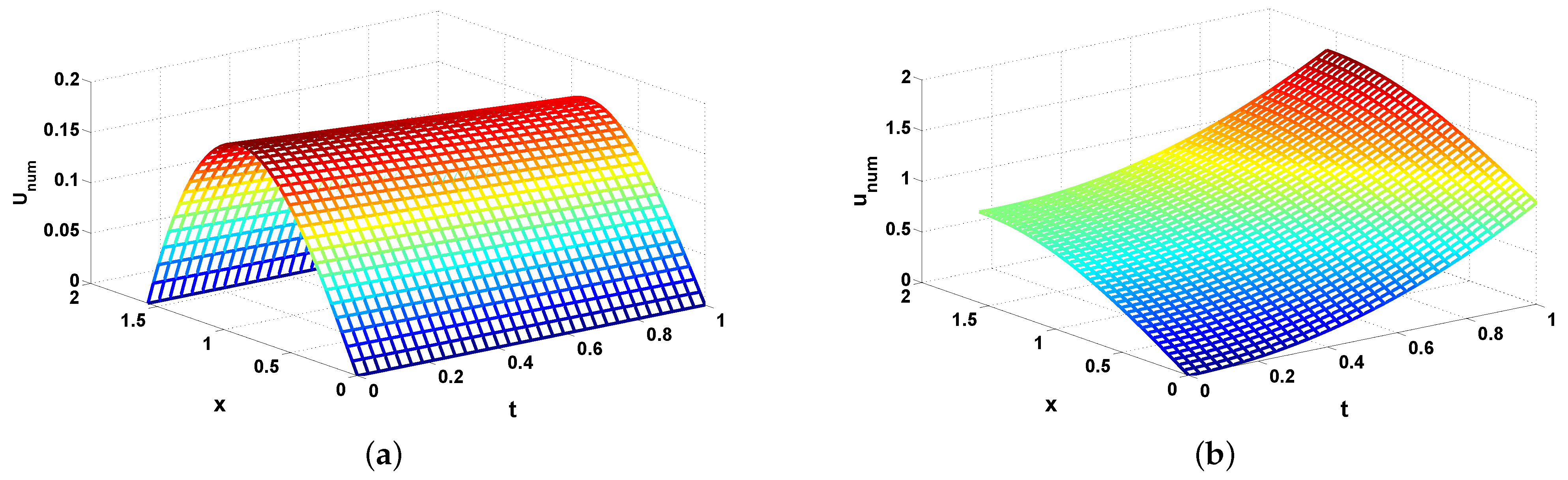
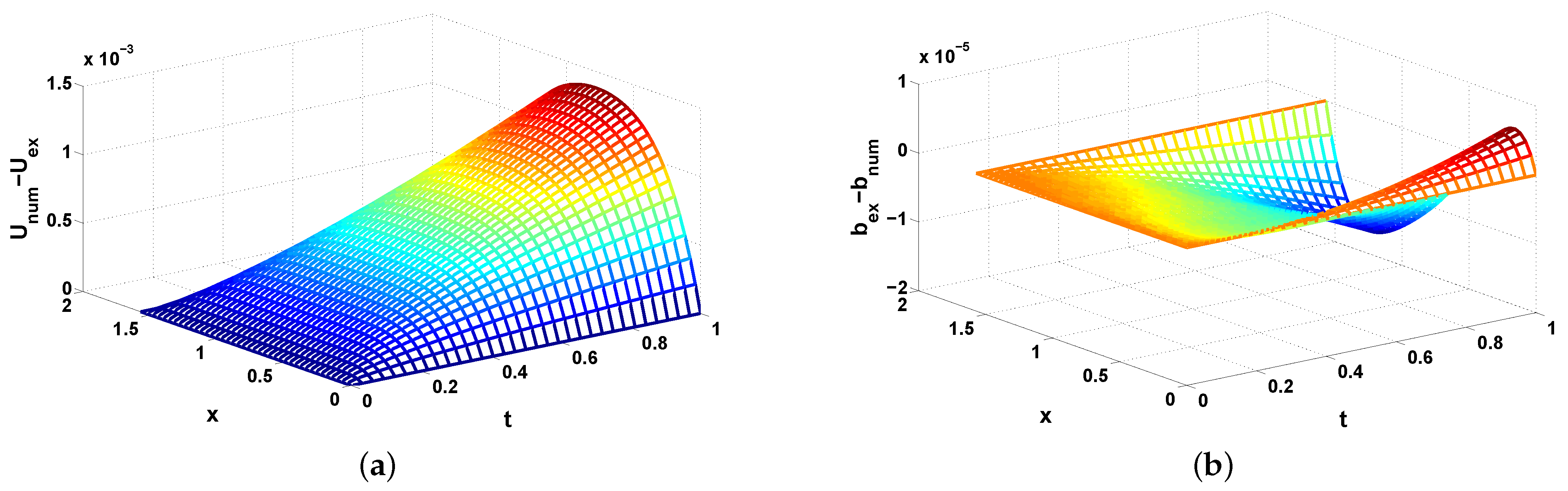
7.1. Inverse Problem without Noise

First, we solve the problem with the integral measurements, taken directly from (53). In Table 1 the results of mesh refinement analysis are presented in the case of $\nu =0.1$, ${\nu }_m=0.2$, $c=1$, $X=\pi /2$, and $T=1$. Theoretically, the linearized finite difference scheme for the direct problem is of second order with respect to time and to space; see [28]. But, due to the first order of the approximations of $U_x(X,t)$ and $U_x(0,t)$, the proposed algorithm leads to first order both for U, b and also for $f\left(t\right)$. The numerical results confirm the theoretical rate of convergence, i.e., $O(\tau +h)$ for the flow velocity $u(x,t)$ and for the magnetic field $B(x,t)$.

Table 1. The error in maximum norm of the flow velocity $u(x,t)$, the magnetic field $B(x,t)$, and the source function $f\left(t\right)$, obtained for $\nu =0.1$, ${\nu }_m=0.2$, $c=1$, $X=\pi /2$, and $T=1$.

		u			B			f
$\mathit{M}$	$\mathit{N}$	${\mathit{err}}_{\mathit{u}}$	Ratio	Order	${\mathit{err}}_{\mathit{B}}$	Ratio	Order	${\mathit{err}}_{\mathit{f}}$	Ratio	Order
5	5	9.2310e-03	-	-	6.5473e-04	-	-	1.1485e-02
10	10	5.0943e-03	1.81	0.86	1.6591e-04	3.95	1.98	6.1159e-03	1.88	0.91
20	20	2.6823e-03	1.90	0.93	4.5833e-05	3.60	1.85	3.1974e-03	1.91	0.94
40	40	1.3803e-03	1.94	0.96	1.6712e-05	2.72	1.45	1.6416e-03	1.95	0.96
80	80	7.0073e-04	1.97	0.98	7.1775e-06	2.32	1.21	8.3274e-04	1.97	0.98
160	160	3.5312e-04	1.98	0.99	3.3274e-06	2.14	1.11	4.1952e-04	1.99	0.99

Shown in Figure 1a is the the numerical solution $U_{num}$ for the corresponding problem (17), (18) and shown in Figure 1b is the numerical values of the flow velocity $u(x,t)$ of the original system (1)–(4), (7) for $N=40$ and $M=32$. In Figure 2a the error $U_{ex}-U_{num}$ and in Figure 2b) the error $b_{ex}-b_{num}$ are depicted for the same values of the mesh parameters. It is clear to see the good approximation of the numerical solution to the exact one.

Figure 1. The numerical solutions for $M=32$, $N=40$: (a) $U_{num}$; (b) $u_{num}$.

Figure 2. Mesh parameters $M=32$, $N=40$: (a) The error in maximum norm for the flow velocity $U(x,t)$; (b) The error in maximum norm for the magnetic field $b(x,t)$.

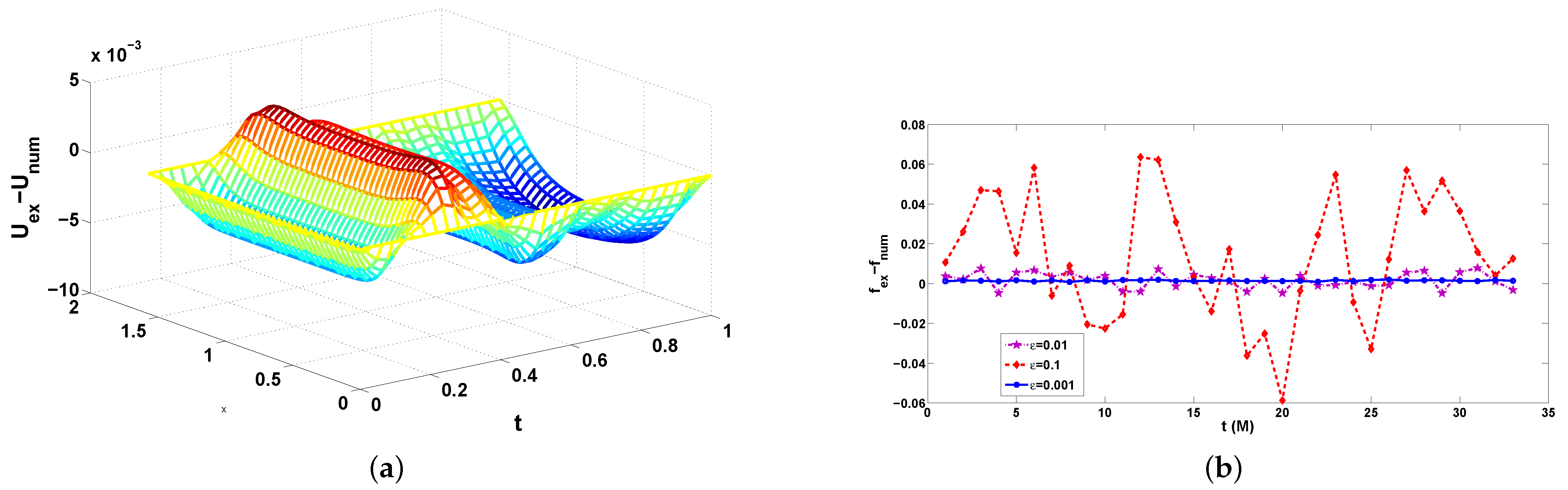
7.2. Inverse Problem with a Noise

Measurements are usually made with devices that allow errors. For this reason, we now consider the same problem, but with randomly perturbed integral measurements $E\left(t\right)$ with a noise:

$$\overline{E}\left(t^j\right)=E\left(t^j\right)+ϵ\sigma \left(j\right);j=0,1,\dots ,M,$$

where $E\left(t^j\right)$ is estimated using (53), $ϵ$ is the amplitude of the noise in the measurements, and $\sigma =\left\{\sigma \right(0),\dots ,\sigma (M\left)\right\}$ is a random vector uniformly distributed in the interval $(-1;1)$. In Table 2, for the case $\nu =0.1$, ${\nu }_m=0.2$, $c=1$, $X=\pi /2$, and $T=1$, the errors in maximum norm of the flow velocity $u(x,t)$, the magnetic field $B(x,t)$, and the unknown function f with a measurement noise are presented for different values of the parameter $ϵ$. The results show that the errors of the flow velocity $u(x,t)$, the magnetic field $B(x,t)$, and the unknown function $f\left(t\right)$ depend weakly on the amplitudes of the deviations in the measurements as opposed to the results obtained in [28].

Table 2. The error in maximum norm of the flow velocity $u(x,t)$, the magnetic field $B(x,t)$, and the unknown function f for Example 2, with measurement noise of amplitude $ϵ$, for $M=40$ and $N=40$.

ffl	0	0.0005	0.001	0.01	0.1
u	1.3803e-03	1.3638e-03	1.5238e-03	2.1379e-03	1.6747e-02
B	1.6712e-05	1.6546e-05	1.6297e-05	2.5556e-05	1.6864e-04
f	1.6416e-03	1.8412e-03	1.9766e-03	7.8766e-03	6.8009e-02

The results of the numerical computations (made by Matlab random generator) with additional perturbation with a noise $ϵ$ are presented in Figure 3 with mesh parameters $M=32$ and $N=40$: (a) the error of $U_{ex}-U_{num}$ and $ϵ=0.1$; (b) the error $f_{ex}-f_{num}$: $ϵ=0.001$ (solid blue line, circles); $ϵ=0.01$ (dash-dot magenta line, stars); $ϵ=0.1$ (dash red line, diamonds). It is clear to see that the noise in the measurements leads to the oscillations in the errors of the computed solutions.

Figure 3. Inverse problem with noise, mesh parameters $M=32$, $N=40$: (a) the error of $U_{ex}-U_{num}$ and $ϵ=0.1$; (b) the error $f_{ex}-f_{num}$: $ϵ=0.001$ (solid blue line, circles); $ϵ=0.01$ (dash-dot magenta line, stars); $ϵ=0.1$ (dash red line, diamonds).

8. Conclusions

In this paper, inverse problems in a 1-D magnetohydrodynamic flow system are investigated. The main idea is to transform the coefficient and source inverse problems into nonclassical forward problems. A loaded equation method is then used to estimate an unknown time-dependent convection coefficient and source. In this inverse problem, two integral observations are placed when both functions are unknown. Implicit finite difference schemes are used to solve the differential problem, and efficient decomposition algorithms to solve nonlocal difference problems are proposed. Numerical test examples with and without noise in the measurements are discussed. The results obtained by the loaded equation technique are more stable than the results in the conference paper [28], where after semi-discretization in time, another linearization technique based on the unknown coefficient and source functions was used.

References

- Alifanov, O.M.; Artyukhin, E.A.; Rumyantsev, S.V. Extreme Methods for Solving Ill-Posed Problems with Applications to Inverse Heat Transfer Problems; Begell House: New York, NY, USA; Wallingford, UK, 2015. [Google Scholar]
- Canon, J.R.; Van Der Hoek, J. Diffusion subject to the specification of mass. J. Math. Appl. 1986, 115, 517–529. [Google Scholar] [CrossRef]
- Kabanikhin, S.I. Inverse and Ill-Posed Problems Theory and Applications; Walter de Gruyter: Berlin, Germany, 2011. [Google Scholar]
- Krukovskiy, A.J.; Poveschenko, J.A.; Podruga, V.O. Convergence of some iterative algorithms for numerical solution of two-dimentional non-stationary problems of magnetic hydrodynamics. Math. Model. 2023, 35, 57–74. (In Russian) [Google Scholar]
- Ladyzhenskaia, V.A.; Solonnikov, V.A.; Ural’tceva, N.N. Linear and Quasi-linear Equations of Parabolic Type; American Mathematical Society: Providence, RI, USA, 1986. [Google Scholar]
- Samarskii, A.A.; Vabishchevich, P.N. Numerical Methods for Solving Inverse Problems of Mathematical Physics; Walter de Gruyter: Berlin, Germany, 2007. [Google Scholar]
- Vabishchevich, P.N.; Vasil’ev, V.I. Computational determination of the lowest order coefficient in a parabolic equation. Dokl. Math. 2014, 89, 179–181. [Google Scholar] [CrossRef]
- Vabishchevich, P.N.; Vasil’ev, V.I. Computational algorithms for solving the coefficient inverse problem for parabolic equations. Inv. Probl. Sci. Eng. 2016, 24, 42–59. [Google Scholar] [CrossRef]
- Ashyraliev, A.; Sazaklioglu, A.V. Investgation of a time-dependent source identification with integral overdetermination. Numer. Funct. Anal. Optim. 2017, 38, 1276–1294. [Google Scholar] [CrossRef]
- Borzi, A. Modelling with Ordinary Differential Equations. A Comprehensive Approach; Chapman and Hall, CRC Press: Boca Raton, FL, USA, 2020. [Google Scholar]
- Georgiev, S.G.; Vulkov, L.V. Computational recovery of time-dependent volatility from integral observations in option pricing. J. Comput. Sci. 2019, 39, 101054. [Google Scholar] [CrossRef]
- Glotov, D.; Hames, W.E.; Meir, A.J.; Ngoma, S. An integral constrained parabolic problem with applications in thermochronology. Comput. Math. Appl. 2016, 71, 2301–2312. [Google Scholar] [CrossRef]
- Glotov, D.; Hames, W.E.; Meir, A.J.; Ngoma, S. An inverse diffusion coefficient problem for a parabolic equation with integral constraint. Int. J. Numer. Anal. Model. 2018, 15, 552–563. [Google Scholar]
- Evans, L.C. Partial Differential Equations, 2nd ed.; Graduate Studies in Mathematics 19; American Mathematical Society: Providence, RI, USA, 2010. [Google Scholar]
- He, Y. Unconditional convergence of the Euler semi-implicit scheme for the three dimensional incompressible MHD equations. IMA J. Numer. Anal. 2015, 33, 767–801. [Google Scholar] [CrossRef]
- Isakov, V. Inverse Problems for Partial Differential Equations, 2nd ed.; Springer: New York, NY, USA, 2006. [Google Scholar]
- Landau, L.D.; Bell, J.; Kearsley, M.; Pitaevski, L.; Lifshitz, E.; Sykes, J. Electrodynamics of Continuous Media; Elsevier: Amsterdam, The Netherlands, 2013; eBook ISBN 9781483293752. [Google Scholar]
- Nguyen, T.N.O. Source identification for parabolic equations from integral observations by the finite difference splitting method. Acta Math. Vietnam. 2024, 49, 283–308. [Google Scholar]
- Samarskii, A.A.; Nikolaev, E.S. Numerical Methods for Grid Equations: Volume I Direct Methods; Birkhäuser Verlag: Berlin, Germany, 1989. [Google Scholar]
- Slodicka, M.; Seliga, L. Identification of memory kernels in hyperbolic problems. J. Comp. Appl. Math. 2017, 311, 618–629. [Google Scholar] [CrossRef]
- Tsyba, V.; Chebatorev, A.Y. Optimal control asymptotics of a magnetohydrodynamic flow. Comp. Math. Math. Phys. 2009, 49, 466–473. [Google Scholar] [CrossRef]
- Marchuk, G.I. Adjoint Equations and Analysis of Complex Systems; Kluwer Acad. Publishers: Dordrecht, The Netherlands, 1995. [Google Scholar]
- Koleva, M.N.; Vulkov, L.G. A Galerkin finite element method for reconstruction of time-dependent convection coefficients and source in a 1-D model of magnetohydrodynamics. Appl. Sci. 2024, 14, 5949. [Google Scholar] [CrossRef]
- Ren, Z.; Guo, S.; Li, Z.; Wu, Z. Adjoint-based parameter and state estimation in 1-D magnetohydrodynamics (MHD) flow system. J. Optim. Manag. Optim. 2018, 14, 1579–1594. [Google Scholar] [CrossRef]
- Yu, P.X.; Tian, Z.F. Comparison of the simplified and full MHD models for laminar incompressible flow past a circular cylinder. Appl. Math. Model. 2017, 41, 143–163. [Google Scholar] [CrossRef]
- Khankishiyev, Z.F. Solution of one problem for linear loaded parabolic type differential equation with integral conditions. Adv. Math. Mod. Appl. 2022, 7, 178–190. [Google Scholar]
- Vabishchevich, P.N.; Klibanov, M.V. Numerical identification of the leading coefficient of a parabolic equation. Differ. Equ. 2016, 52, 855–862. [Google Scholar] [CrossRef]
- Kandilarov, J.; Vulkov, L. Simultaneous numerical reconstruction of time-dependent convection coefficient and source in magnetohydrodynamics flow system. In Proceedings of the 16th Annual Meeting of the Bulgarian Section of SIAM, (BGSIAM’21) (to Appear), Sofia, Bulgaria, 21–23 December 2021. [Google Scholar]
Disclaimer/Publisher’s Note: The statements, opinions and data contained in all publications are solely those of the individual author(s) and contributor(s) and not of MDPI and/or the editor(s). MDPI and/or the editor(s) disclaim responsibility for any injury to people or property resulting from any ideas, methods, instructions or products referred to in the content. |
© 2024 by the authors. Licensee MDPI, Basel, Switzerland. This article is an open access article distributed under the terms and conditions of the Creative Commons Attribution (CC BY) license (https://creativecommons.org/licenses/by/4.0/).