Abstract
The discrete cosine transform (DCT) is widely used for image and video compression. Lossy algorithms such as JPEG, WebP, BPG and many others are based on it. Multiple modifications of DCT have been developed to improve its performance. One of them is adaptive DCT (ADCT) designed to deal with heterogeneous image structure and it may be found, for example, in the HEVC video codec. Adaptivity means that the image is divided into an uneven grid of squares: smaller ones retain information about details better, while larger squares are efficient for homogeneous backgrounds. The practical use of adaptive DCT algorithms is complicated by the lack of optimal threshold search algorithms for image partitioning procedures. In this paper, we propose a novel method for optimal threshold search in ADCT using a metric based on tonal distribution. We define two thresholds: pm, the threshold defining solid mean coloring, and ps, defining the quadtree fragment splitting. In our algorithm, the values of these thresholds are calculated via polynomial functions of the tonal distribution of a particular image or fragment. The polynomial coefficients are determined using the dedicated optimization procedure on the dataset containing images from the specific domain, urban road scenes in our case. In the experimental part of the study, we show that ADCT allows a higher compression ratio compared to non-adaptive DCT at the same level of quality loss, up to 66% for acceptable quality. The proposed algorithm may be used directly for image compression, or as a core of video compression framework in traffic-demanding applications, such as urban video surveillance systems.
1. Introduction
The smart city is a popular concept in applied computer science. The development of smart city subsystems requires the integration of multiple information and communication technologies, including Internet of Things and computer vision, which would support city infrastructure. Closed-circuit television (CCTV) systems play an important role in the concept of the smart city, especially considering life safety issues. Ensuring that a city has full CCTV coverage and high footage quality is fundamental to ensuring safe road networks, employing unmanned vehicles and reporting road traffic incidents. For example, in cities with the most developed video surveillance systems, the density exceeds 400–500 cameras per square kilometer [1]. However, with the increase in the number of video cameras and other image information sources together with the improvement of video quality characteristics, problems arise associated with the need to transmit, store and process huge amounts of data. For example, in the overview observation mode, the camera generates an average video data stream at a rate of 6 Mbit/s. For 400 cameras, the rate of generated data is 300 MB/s, i.e., almost 18 GB per minute and over 1 TB per hour. With the need for transmitting, processing and storing such volumes of video data, it is important to apply efficient image and video compression methods. Various image compression and restoration algorithms have been extensively studied by scholars for the last few decades. Algorithms such as JPEG [2,3], WebP [4,5], BPG [6,7] and FLIF [8] have been developed and enhanced in the last few decades. When performing compression of the video stream from CCTV cameras, the following features of video information should be taken into account:
- Most of the frame is often occupied by a static background (sidewalk, buildings, advertisements, temporary banners, sky, etc.);
- The intensity and density of traffic flows change over time;
- In the absence of movement between frames, there is a high degree of correlation over time;
- The contrast between objects in video frames and the background is relatively low.
Practical solutions in image compression algorithms suggest that the original image can be compressed into a power-2 square before applying DCT and then fragmented, typically into 8 × 8-pixel squares. In standard DCT, after fragmentation, the transformation is applied separately to each fragment. The authors of [9,10] provide alternative approaches to interpreting quadtree decomposition. They propose, instead of applying transformation to the blocks themselves, to take a pixel from each block to form sub-ranges of the original image and then transform the resulting sub-ranges. This leads to better spectral representation since each sub-band is essentially a smaller version of the original image and resolves the problem of blocking artifacts from appearing in the image. However, this approach affects the natural properties of original images, which typically have smooth transitions between adjacent pixels, resulting in a convenient quantization of the spectrum that retains most of the energy at low frequencies.
After converting the sub-bands, the resulting DCT coefficients are quantized, i.e., divided by a certain number or separated into elements of the quantization matrix. At the quantization stage, there is a loss of image quality, since some integer DCT coefficients become equal to zero or different from the original value. However, this allows one to compress the resulting image more extensively. The stronger the quantization of coefficients is, the greater the loss of quality will be and the higher the compression level that can be achieved.
Adaptive discrete cosine transform is a modification of DCT based on the application of variable-sized tiles to the original image, which is split before performing the transform [11,12,13,14,15]. The sub-band approach described earlier is difficult to implement in ADCT and would lose many of its benefits such as the elimination of blocking artifacts, so the standard DCT fragmentation interpretation can be henceforth used. ADCT may imply a limited set of tile sizes, such as using only a set of 16 × 16-, 8 × 8- or 4 × 4-pixel sizes, or simply recursively dividing the maximum possible size to 2 × 2 pixels, which is the minimal DCT input. However, using tiles smaller than 8 × 8 produces poor inefficient results, so in further work the maximum tile size is considered unlimited, up to the largest power of two that fits in the image size, and the minimum tile size is 8 × 8, as in JPEG. This means that the goal of the fragmenting algorithm is to compress the image into the largest tiles possible before applying the transform.
To assess the need for fragments’ separation, a function is required to determine the amount of details in the fragment. It should ensure accurate and efficient fragmentation when performing ADCT. The simplest solution is to convert the image to grayscale and treat the image fragment as a one-dimensional array of pixels of various brightness. By analyzing the statistical properties of brightness values, it is possible to estimate the change in brightness of pixels within a fragment. A naive approach would be to calculate the root mean square error (RMSE) or similar statistical metrics for the brightness of the pixels. A lower RMSE here should mean less variation in tone, closer to a solid color, and therefore contains less noticeable details, and vice versa. RMSE by definition takes into account the size of the input data, i.e., the tile size.
However, the straightforward application of RMSE to pixel tones has a major drawback: the tonal distribution of the image is sensitive to the changes in the tonal range. Expanding the tonal distribution of an image, for example, by equalizing the histogram, does not increase the level of detail, it only enhances its visibility. The same applies to narrowing the tonal distribution, unless this leads to an overlap of tones and changes in the shape of the tonal histogram. In this article, we use the value of tonal distribution variance (TDV) and its inverted value (ITDV) to determine the ADCT thresholds. The thresholds are between 0 and 1 for any image size and tonal range. This enables convenient fragmentation during ADCT while preserving its accuracy regardless of the image properties.
Only monochrome, grayscale images are researched in this paper. The proposed algorithm can also be applied to the colored images by transforming the color channels. Since the human eye is less sensitive to changes in color compared to the changes in brightness, the target quality can be even lower for the color channels.
In Table 1, we present a summary of popular existing compression algorithms and compare the proposed implementation of adaptive discrete cosine transform to them.

Table 1.
ADCT compared to other algorithms.
The research into adaptive discrete cosine transformation aims to prove the usefulness of adaptive elements in existing compression methods, such as JPEG2000, MPEG, etc., comparing it with the conventional, non-adaptive transformation that underlies the operation of most algorithms. Considering the abovementioned statements, the contribution of the paper is as follows:
- We introduce and analyze adaptive DCT based on two thresholds (named pm and ps), explained in detail in the paper further, aiming for an optimal tradeoff between quality and compression. The pm threshold determines averaging the fragment to a solid color, and the ps threshold sets the criterion for splitting the fragments.
- We find the optimal pm and ps values corresponding to the target multi-scale structural similarity index measure (MS-SSIM) and compression ratio. MS-SSIM measures the perceptual difference between two similar images, i.e., input and decompressed images, at different scales [18,19,20].
- We compare the proposed ADCT with standard DCT and find numerical estimates of the compression ratio improvement.
The rest of the paper is organized as follows. In Section 2, we describe a novel approach for optimizing the adaptive discrete cosine transform based on the two introduced thresholds. The improvement in the image compression ratio value is shown in Section 3. A summary of the results obtained is given in Section 4. Appendix A contains additional illustrations, plots and tables obtained during the experiments.
2. Materials and Methods
2.1. Earlier Adaptive DCT
Research on adaptive discrete cosine transformation dates back to the 1980s. The earliest implementations of the algorithm achieved bitrates as low as 0.5 bits per pixel while maintaining the compression practically losslessly [21,22]. The early developments were primarily dedicated not to the splitting of the images into fragments of variable size but to the encoding.
In video compression, there are developments dating back to the 20th century as well. For example, adding variable length to three-dimensional discrete cosine transform (3D DCT) blocks, implementing temporal adaptivity, has allowed the achievement of an astonishing 0.1 bit per pixel rate on average for a video without a significant loss in quality (bottom right frame in Figure 1) [23].
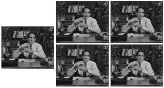
Figure 1.
Examples of video compression using 3D DCT, comparing the original video frame and various compression techniques, with variable-temporal-length 3D DCT implementations in the bottom row, clearly showing its superiority.
More recent implementations of 3D adaptive DCT claim to be superior to common compression methods. It is also said to reduce the complexity of the calculations, allowing them to be implemented easily in hardware [24]. The lack of temporal dimension efficiency of regular 3D DCT is compensated for by adaptivity, such as presented in Figure 2, and is described as surpassing MPEG in both bitrate and efficiency. Mentions of thresholds being used in adaptive fragmenting quadtree building are first found in the abovementioned work.

Figure 2.
Example of adaptive 3D DCT in a video frame, showcasing both fragmenting and replacing entire fragments with their average tones.
However, methods to calculate the adaptive fragmenting thresholds have never been described thoroughly. Our work aims to provide the foundation for implementing adaptivity techniques in compression methods by describing how to obtain the threshold values.
2.2. Proposed Adaptive DCT Algorithm
Let us represent the image as a function g:
where x and y are the coordinates of an image pixel. The restored image after compression with thresholds and can be defined as follows:
Let us introduce an evaluation function f. We will assume that it possesses a local minimum at certain optimal threshold values pm, ps. Thus, the mathematical definition of the chosen problem is to find the value
for each image. Then, a data-fitting approximation of arbitrary order is applied to the set of “original level of image detail–optimal threshold value” pairs for each of the two thresholds.
It should be noted that, when the value of the function f is close to the local minimum, the value of MS-SSIM approaches 1. The standard SSIM formula is as follows:
where is the pixel sample mean of x, the pixel sample mean of y, the variance of x, the variance of y, the covariance of x and y, two variables to stabilize the division with weak denominator, and L the dynamic range of the pixel values, L = 255, and . MS-SSIM is a composition of several SSIM measurements taken for downscaled versions of the image. The relative importance coefficients for the 5 measurements are default and as such 0.0448, 0.2856, 0.3001, 0.2363 and 0.1333, respectively, for the scales from 1 to 5 [18].
To set up the optimization process, three quality levels were derived. They are different in the target MS-SSIM (minimum acceptable value during optimization) and quantization values:
- High level corresponds to target MS-SSIM = 0.98, quantization value 10 and typically minor degradation;
- Medium level: target MS-SSIM = 0.90, quantization value 30, noticeable degradation in quality, but many details are preserved;
- Low level: target MS-SSIM = 0.80, quantization value 100, significant quality degradation while preserving the most detailed areas.
An example of adaptive DCT is shown in Figure 3.
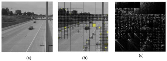
Figure 3.
Example of adaptive discrete cosine transform: (a) original image; (b) quadtree grid on the image, yellow color marks the solid color fragments; (c) adaptive discrete cosine transform spectrum of the image (brightened up for clarity).
Figure 3 shows the basic principles of constructing an image quadtree via the proposed method.
In this study, we will not use RMSE to determine ADCT thresholds and instead use the values of TDV and ITDV, because expanding the tonal distribution of an image increases tone visibility and does not directly affect detail while changing the RMSE value. Vice versa, narrowing the tonal range does not increase detail, yet it changes the RMSE value as well. Examples of tonal histograms of images are shown in Figure 4.
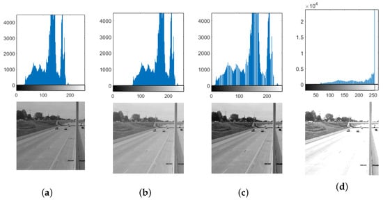
Figure 4.
Examples of image histograms: (a) histogram of the original image; (b) histogram after increasing the brightness by 40%; (c) histogram after normalization, i.e., extending it to the entire 0–255 spectrum width; (d) histogram after multiplying the brightness by 2, resulting in a “whiteout” (overexposure).
One can see that the amount of detail cannot be measured by calculation using actual tone values: the RMSE will change as the histogram changes. However, the image histogram can be used for its original purpose, namely visualizing the tonal distribution. Making an array out of pixel brightness values associated with a histogram results in an array of 256 elements, each one corresponding to a pixel brightness value. Each element is then assigned the number of corresponding pixels of the image. The order of these elements does not affect the calculation of the mean value and the variance, so changes in brightness or histogram normalization also do not affect the calculations.
The root mean square error can be calculated for this distribution of 256 tone values. However, a more elegant and efficient approach by calculating tonal distribution variance is illustrated further.
For an input image or image fragment consisting of pixels, the average tonal distribution (TD) value is , since the tonal values of the pixels are arbitrarily distributed among the 256 elements.
Therefore, the variance can be calculated as follows:
where i is the pixel tone index, is the total number of pixels in the image or fragment and TD is the tonal distribution array, consisting of 256 counts of pixels of specific brightness. For example, is the number of black pixels and is the number of white pixels in the fragment or image. Examples of this distribution can be observed in Figure 4.
Thus, the variance will be sensitive to the input size since there are more pixel hue values in the distribution. However, by instead dividing the sum of squared errors by , a normalized value between 0 and 1 is obtained, regardless of the value of L. A value of 0 means zero variance in the distribution, indicating a completely uniform tonal distribution, and 1 corresponds to the maximum possible variance, where one solid tone fills one tonal distribution array element and leaves other elements empty.
Let us prove the abovementioned statement. If is the mean TD value, there is only one tone array element filled with L pixels and the rest are empty. Then, the sum of squared errors is
where the first term is the squared error between the mean and the maximum value of the diapason and the second term is the squared error between the mean and the zeros for the remaining 255 out of 256 tones.
This expression is equal to
Therefore, dividing the squared errors’ sum by
instead of 256 provides a more practically applicable and generalized value. This lies between 0 and 1 and is derived from a sum of squared values. To make the distribution practical and gradual we take a square root from the quotient, without changing the properties of the normalized value. Since the value correlates to variance, we call it tonal distribution variance (TDV). The resulting formula is as follows:
For comparison, the RMSE of an image fragment can be calculated with the following formula:
Tonal distribution variance directly correlates with RMSE up to a constant multiplier. However, multiplying or dividing pixel brightness values changes the tonal range and, consequently, the RMSE value. However, the TDV remains constant unless the multiplication makes pixels reach maximum brightness or a division forces individual brightness values to 1. This clearly demonstrates that TDV is more versatile than RMSE due to being independent of the tonal range of the image.
Thus, using this metric allows one to safely set the thresholds inside the 0–1 range for arbitrary image size and tonal range.
The first threshold ps (split) determines whether the image fragment should be further split into four quadrants. If the TDV of a fragment is below ps, then the tonal distribution of the fragment is supposed to be less uniform, contain more tones and, probably, more details, so it is logical to split it to preserve details after performing a discrete cosine transform.
The second threshold pm (mean) determines whether the fragment appears monochromatic enough (if TDV is above pm) to be replaced by a single average value of its brightness. The result is the highest possible level of compression since there is only one non-zero DCT coefficient left in the spectrum. Having mean-value tiles does not detract too much from image quality as long as they are small enough not to affect valuable details. For our purposes, it is acceptable to paint unimportant details, like road surface or sky, in solid color, as long as the resulting quality is sufficient. Solid color fragments are demonstrated in Figure 5.
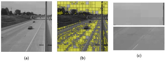
Figure 5.
Example of solid color fragments: (a) processed image; (b) processed image: solid color fragments are marked with yellow; (c) close-ups of the sky and the road surface demonstrate little impact on the overall perception unless zoomed in.
When constructing a quadtree using the abovementioned thresholds, the fragment is first tested with the threshold pm and only then checked for further fragmentation. This means that for each fragment there are three possible outcomes:
- Replacing with a solid color if its TDV is higher than pm;
- Leaving as is if its TDV is between pm and ps;
- Splitting into four sub-fragments if its TDV is below ps.
Tonal distribution variance appeared to be in the range between 1/15 and 1/10 for many of the traffic images in our experiments. Meanwhile, there are cases where completely solid color frames possess a TDV equal to 1. For convenience and visibility, further on we used the inversion of TDV, called ITDV, to display the distribution of frames with more convenient numbers instead of fractions:
The majority of the frames are then found in the 10–15 ITDV range.
We introduce an optimization process consisting of the following steps: choosing pairs of threshold ADCT values, constructing quadtrees using them, performing discrete cosine transform on their fragments and checking whether the results satisfy certain requirements. The threshold values are optimized for images with various original ITDVs, i.e., the tonal distribution variance is calculated for the entire original image, as we assume it is an acceptable measure of image detail. Optimal thresholds should provide maximum compression efficiency while preserving a certain level of image quality.
The example shown in Figure 6 illustrates a quality comparison of compressed images with three distinct levels.
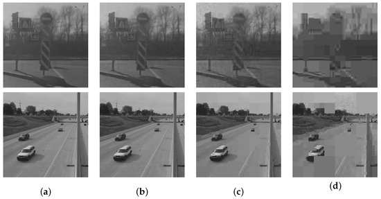
Figure 6.
Image quality comparison: (a) the original images; (b) high-quality ADCT; (c) medium-quality ADCT; (d) low-quality ADCT.
For simplicity, the compression ratio is calculated here as a ratio between non-zero DCT coefficients and the total number of coefficients. It does not necessarily portray the actual compression ratio of the stored file, but we consider it sufficiently suitable for this study. Given the appropriate data compression methods for the pixel information, such as run-length encoding, the chosen compression ratio metric allows for good relative comparison between methods. This frees us from the burden of describing a full-scale compression method to implement and measure bits per pixel metric or similar. For example, to compare the performance of ADCT with regular JPEG, one can set appropriate thresholds to split the image into 8 × 8 tiles without creating solid color fragments, mimicking regular DCT, and then compare the resulting ratios.
The optimization process consists of three levels of optimal value search for the ps and pm thresholds. Given that TDV is normalized between 0 and 1, we can evaluate the result of compression with different pairs of threshold values from this diapason, increasing the precision of the search step by step.
At the first level of optimization, pairs of threshold values are evaluated with 0.1 accuracy (0.05:0.05, 0.05:0.15, …, 0.95:0.95). For each pair, a quadtree is constructed for the tested image and ADCT is performed to obtain the compression ratio and MS-SSIM between the result and the original image since the latter must be above the minimal threshold for the chosen compression quality. Then, a pair with the best resulting compression ratio is chosen for the next level of search with higher accuracy (0.01, then 0.001). New values are searched for in the vicinity of the previous optimal values. As a result, optimal values are obtained with an accuracy of 3 decimal digits.
A visual representation of the search algorithm is shown in Figure 7. The grid represents the pairs of threshold values. The colors, from blue to red, represent the resulting compression ratio value after ADCT: blue represents the minimum value on the search level and red represents the maximum value. Black represents invalid threshold value pairs or that resulting MS-SSIM is below the target value for the chosen quality. A threshold value pair with the biggest compression ratio on one level is searched through at higher precision at the next level, with 3 levels of precision in total. If there are threshold value pairs with similar compression ratios, one with the best MS-SSIM is chosen. However, an equal compression ratio usually means equal quadtree structure and equal MS-SSIM; the first pair by order is chosen then.

Figure 7.
Flowchart of the optimization process; the grid is the search area; each grid cell is a pair of threshold values.
The image illustrates the search process on all three levels: first the 0.25:0.35 pair is chosen out of the 0.05:0.05 (top left) to 0.95:0.95 (bottom right) field, then 0.27:0.31 is chosen from the 0.21:0.31–0.30:0.40 field, then the leftmost red cell representing 0.267:0.306 is chosen from the 0.266:0.306–0.275:0.315 field.
3. Results and Discussion
To process the experimental data and search for optimal ADCT thresholds, we developed a software implementation of the corresponding algorithm written in C++. The quadtree division algorithm is deterministic by nature because no random values are used, meaning the quadtree will not change if the same parameters and inputs are used. The discrete cosine transform is implemented using the row–column method, which decomposes the original two-dimensional transform into a sequence of two one-dimensional transforms, greatly reducing the complexity of the algorithm. Since the optimization is performed independently for each image in the set, the process can be defined as parallel, allowing parallel computation to be easily implemented using the OpenMP interface and greatly speeding up the calculations.
To evaluate the experimental results quantitatively, we define the approximate compression ratio (CR), calculated by the following formula:
Every fragment of the compressed image consists of a DC (so-called direct current) coefficient—the first coefficient responsible for the mean color part of the fragment, practically always the biggest, non-zero AC (alternating current) coefficients usually responsible for low cosine frequencies, and zero AC coefficients that have been reduced or rounded to zero, usually those responsible for high frequencies. Removing the high-frequency coefficients leads to losing information on details but also provides most of the compression.
The DC coefficient is always present and requires a constant number of bits for encoding, depending on the quantization factor. Zero AC coefficients can be encoded with run-length encoding using the zigzag pattern with just a single number—the number of these zero coefficients. Thus, the amount of non-zero AC coefficients arguably plays the most important role in the resulting bitrate, since it requires a variable amount of encoding instances, unlike the two previous categories of DCT coefficients. Apart from the DC coefficient, the run-length encoding of the zero coefficients and a technique to encode the structure of the quadtree, we consider the ratio between the non-zero coefficients and their total amount a fitting metric to express the quantity of compression. If all the techniques employed in existing algorithms such as JPEG, e.g., Huffman coding, are applied to ADCT, the resulting bits per pixel metric will mostly depend on the difference between the regular DCT’s and the adaptive DCT’s compression ratios.
As a second quantitative quality metric apart from MS-SSIM, we use peak signal-to-noise ratio (PSNR) for compressed images against the original ones.
It is important to note that, since ADCT results in the construction of a quadtree from power-2-sized fragments, the source images must also be power-2-sized or padded to fit into the required dimensions.
The optimization results are presented in the figures below, where each subplot corresponds to a certain level of image quality.
The results of calculating the optimal threshold values for images with different original ITDVs are shown in Figure 8.
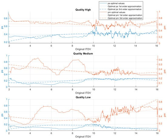
Figure 8.
Optimal threshold values for different original ITDV values of the images.
The resulting distribution for each quality level can be approximated. We tested fitting a linear function and a third-order curve using the least squares method implemented in MATLAB. The threshold searching program was modified to use the resulting threshold functions instead of performing optimization. It outputs MS-SSIM values between the original and compressed image and compares the compression ratios for the linear and the third-order curves. The experimental verification with a test dataset is explained further. As one can see, a decrease in target compression quality not only lowers the thresholds but also creates a gap between them. A decrease in quality also allows less detailed images (with lower original ITDV) to be covered in solid color.
Threshold value approximation equations depending on quality (original image ITDV) are presented in Table 2 and Table 3. Table 2 considers equations of the linear approximation.

Table 2.
First-order threshold value approximation equations.

Table 3.
Third-order threshold value approximation equations.
Table 3 presents equations of the third order.
For experimental verification of our approach, we used a different test dataset of 600 video frames of size 256 × 256 pixels obtained from real highway video footage (Figure 9). The ITDV distribution of the chosen dataset’s frames is shown in Figure 10.

Figure 9.
Examples of the test dataset frames.
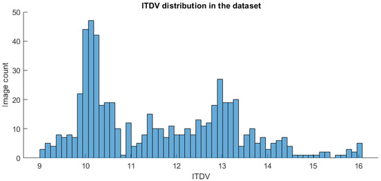
Figure 10.
Distribution of ITDV values through all images of the considered dataset.
The obtained results were compared to the non-adaptive discrete cosine transform such as used in the JPEG algorithm. The graphs in Figure 11 illustrate the dependence between MS-SSIM and the compression ratio of adaptive DCT (ADCT) and conventional DCT (DCT), respectively.
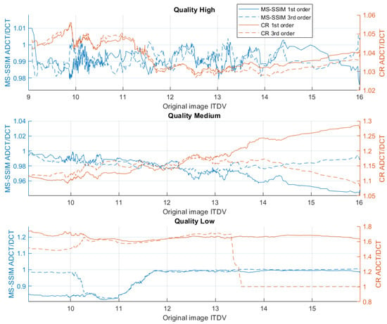
Figure 11.
Comparison of resulting MS-SSIM and compression ratio after ADCT and non-adaptive DCT for ITDV values from 9 to 16.
As we can see from Table 4, lower target quality allows adaptive DCT to better express its advantages. High-quality compression slightly improves the compression ratio over regular DCT (3% higher on average) while preserving the quality (1% lower MS-SSIM on average). Meanwhile, low-quality compression with ADCT on average provides a 66% higher compression ratio with an 8.4% MS-SSIM loss when using the first-order approximation for the threshold values. We can also observe that first-order linear approximation demonstrates higher stability than the third-order curve and provides better results. At low quality, third-order approximation led to ADCT splitting without solid color fragments just like non-adaptive DCT, hence the match in MS-SSIM and CR values. The optimal threshold equations have been tested using the frames from the testing dataset as well as on other images, mainly highway imagery. The comparison between adaptive and non-adaptive DCT is presented for images with various compression qualities in Appendix A.

Table 4.
Summary of the ADCT improvements over regular DCT from graphs above.
We approximated the resulting bitrate (bits per pixel) of the images compressed with ADCT and regular DCT and compared this bitrate against MS-SSIM for both methods. We demonstrate this in Figure 12. As we can see, adaptive DCT becomes more efficient at lower bitrates. It still trades quality for compression but can quickly reach lower bits per pixel values and better compression.
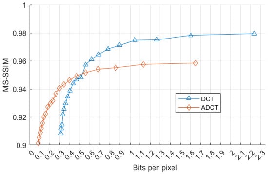
Figure 12.
Graphical comparison of proposed ADCT with non-adaptive DCT in terms of approximated bit rate vs. MS-SSIM.
Using this data, we compared our algorithm to other existing methods [25] and demonstrate it in Figure 13. The comparison does not account for only using static images in H.264. We believe that without motion compensation techniques our algorithm can compete with the existing methods.
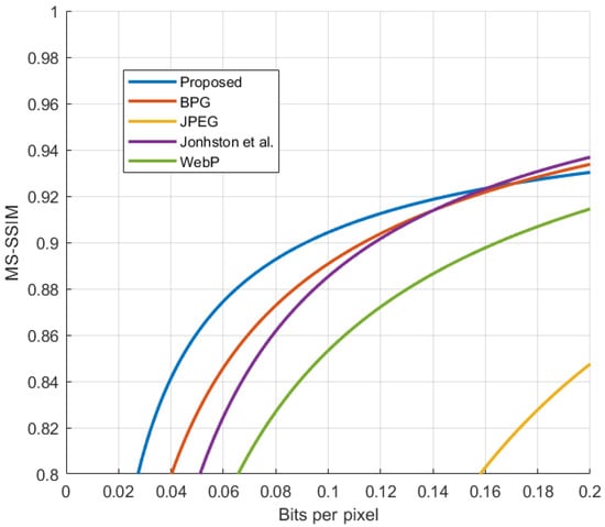
Figure 13.
Comparison [25] with the existing algorithms.
Additionally, the qualitative assessment of ADCT vs. DCT performance throughout the experiment is shown in the tables in Appendix A. An example of better compression of an image using the obtained ADCT threshold values over regular 8 × 8 DCT is shown in Figure 14. A comparison of image compression metrics is shown in Table 5. The threshold values for ADCT are derived from the obtained first-order equations and are as follows: given the original ITDV equals 11.666, with low target quality, ps = 0.112, pm = 0.441.
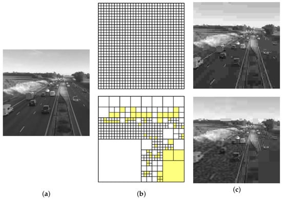
Figure 14.
Advantage in low target quality compression of ADCT over DCT and preservation of information about vehicles in the scene: (a) original image; (b) fragmentation quadtree of ADCT and grid of DCT (yellow fragments are solid color); (c) resulting images (details about car positions are preserved).

Table 5.
Quantitative comparison of image compression in Figure 14.
One can see that an improvement, big or small, in the compression ratio can be observed in all cases. The biggest improvement in compression is seen at the low-quality level for less detailed images. The explanation is that the considered images tend to have larger areas suitable for fitting large fragments of solid color. However, the use of optimal ADCT threshold values can lead to slight drops in the quality measures and overall look of the frame, which would require additional research with a larger dataset and, possibly, additional metrics.
4. Conclusions
In this paper, we presented a novel image compression method based on adaptive discrete cosine transform (DCT) with two quadtree fragmentation thresholds. The superior compression ratio of the optimized method over non-adaptive DCT has been experimentally demonstrated. In particular, we found that the adaptive DCT is most effective when it produces larger fragments of solid color and the target quality is not high, expecting to trade details for compression. By adjusting the defined thresholds, the algorithm finds a sufficient balance between the level of image compression and the retained detail quality, as was measured by the MS-SSIM metric.
The key relations were found between the compression ratio and the quality estimates of the compressed images, such as the amount of detail in the image. In the case of medium compression quality, the increase in the compression ratio reaches 15% on average, which we established by examining a dataset containing 600 images with road traffic scenes. When the image quality is low, the compression ratio of the adaptive DCT outperforms the corresponding value of the conventional DCT by 66%.
Using an equivalent distribution metric for frame temporal correlation could allow extending the proposed adaptive algorithm to the time dimension, improving the compression of the video stream. The implementation of adaptive DCT to video compression is the goal of future research.
Author Contributions
Conceptualization, S.F.; data curation, A.S. and A.V.; formal analysis, A.K. and A.V.; funding acquisition, T.K.; investigation, A.K. and A.S.; methodology, S.F.; project administration, T.K.; software, A.K. and A.Z.; supervision, T.K. and S.F.; validation, A.S. and T.K.; visualization, A.V. and A.Z.; writing—original draft, A.K. and A.S.; writing—review and editing, A.V., A.Z. and T.K. All authors have read and agreed to the published version of the manuscript.
Funding
This study was supported by the Russian Science Foundation (RSF), project 20-79-10334.
Data Availability Statement
The original contributions presented in the study are included in the article; further inquiries can be directed to the corresponding author.
Conflicts of Interest
The authors declare no conflicts of interest.
Appendix A
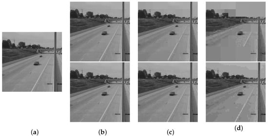
Figure A1.
Highway footage frame test: (a) The original image. (b) High-quality ADCT and DCT. (c) Medium-quality ADCT and DCT. (d) Low-quality ADCT and DCT.

Table A1.
Highway footage frame, original ITDV = 11.63851.
Table A1.
Highway footage frame, original ITDV = 11.63851.
| Quality | MS-SSIM (ADCT/DCT) | CR (ADCT/DCT) | PSNR, dB (ADCT/DCT) |
|---|---|---|---|
| High | 0.986/0.995 | 8.350/7.483 | 39.675/43.559 |
| Medium | 0.939/0.976 | 25.807/18.663 | 33.086/37.150 |
| Low | 0.782/0.899 | 151.661/45.369 | 24.494/31.211 |
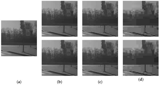
Figure A2.
Recorder footage frame test: (a) The original image. (b) High-quality ADCT and DCT. (c) Medium-quality ADCT and DCT. (d) Low-quality ADCT and DCT.

Table A2.
Recorder footage frame, original ITDV = 13.24893.
Table A2.
Recorder footage frame, original ITDV = 13.24893.
| Quality | MS-SSIM (ADCT/DCT) | CR (ADCT/DCT) | PSNR, dB (ADCT/DCT) |
|---|---|---|---|
| High | 0.987/0.989 | 4.727/4.571 | 40.967/41.978 |
| Medium | 0.947/0.955 | 12.393/11.161 | 33.620/34.908 |
| Low | 0.846/0.8507 | 53.781/36.818 | 28.738/28.842 |
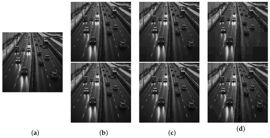
Figure A3.
Dark highway photo test: (a) The original image. (b) High-quality ADCT and DCT. (c) Medium-quality ADCT and DCT. (d) Low-quality ADCT and DCT.

Table A3.
Dark highway photo, original ITDV = 12.14221.
Table A3.
Dark highway photo, original ITDV = 12.14221.
| Quality | MS-SSIM (ADCT/DCT) | CR (ADCT/DCT) | PSNR, dB (ADCT/DCT) |
|---|---|---|---|
| High | 0.989/0.997 | 3.897/3.735 | 37.495/41.521 |
| Medium | 0.955/0.987 | 9.519/8.803 | 31.913/34.188 |
| Low | 0.887/0.936 | 37.186/27.635 | 27.045/27.787 |

Table A4.
Sunny highway photo, original ITDV = 14.02255.
Table A4.
Sunny highway photo, original ITDV = 14.02255.
| Quality | MS-SSIM (ADCT/DCT) | CR (ADCT/DCT) | PSNR, dB (ADCT/DCT) |
|---|---|---|---|
| High | 0.982/0.997 | 2.746/2.644 | 34.892/41.004 |
| Medium | 0.951/0.988 | 5.406/5.066 | 28.827/32.762 |
| Low | 0.911/0.923 | 20.140/16.801 | 25.053/25.388 |
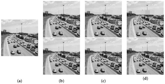
Figure A4.
Sunny highway photo test: (a) The original image. (b) High-quality ADCT and DCT. (c) Medium-quality ADCT and DCT. (d) Low-quality ADCT and DCT.
References
- Bischoff, P. WebP, Surveillance Camera Statistics: Which Are the Most Surveilled Cities? 2023. Available online: https://www.comparitech.com/vpn-privacy/the-worlds-most-surveilled-cities/ (accessed on 13 May 2024).
- Wallace, G. The JPEG algorithm for image compression standard. Commun. ACM 1991, 34, 30–44. [Google Scholar]
- JPEG. WebP, ITU-T T.800 (T.JPEG2000). 2024. Available online: https://handle.itu.int/11.1002/1000/15939 (accessed on 3 March 2024).
- Melenchón Maldonado, J. WebP, a New Web Oriented Image Format. 2010. Available online: http://mosaic.uoc.edu/2010/11/18/webp-a-new-weboriented-image-format-english-version/ (accessed on 16 March 2024).
- Si, Z.; Shen, K. Research on the WebP image format. In Advanced Graphic Communications, Packaging Technology and Materials; Springer: Singapore, 2016; pp. 271–277. [Google Scholar]
- Li, F.; Krivenko, S.; Lukin, V. An approach to better portable graphics (BPG) compression with providing a desired quality. In Proceedings of the 2020 IEEE 2nd International Conference on Advanced Trends in Information Theory (ATIT), Kyiv, Ukraine, 25–27 November 2020; pp. 13–17. [Google Scholar]
- Li, F.; Krivenko, S.; Lukin, V. An Automatic Optimization Method for BPG Compression Based on Visual Perception. In International Scientific-Practical Conference; Springer: Cham, Switzerland, 2021; pp. 213–225. [Google Scholar]
- Sneyers, J.; Wuille, P. FLIF: Free lossless image format based on MANIAC compression. In Proceedings of the 2016 IEEE International Conference on Image Processing (ICIP), Phoenix, AZ, USA, 25–28 September 2016; pp. 66–70. [Google Scholar]
- Jaber, A.K. Low Complexity Embedded Image Compression Algorithm using Subband Coding of the DCT Coefficients. Kufa J. Eng. 2012, 3, 1–16. [Google Scholar]
- Hou, X.; Liu, G.; Zou, Y. Embedded quadtree-based image compression in DCT domain. In Proceedings of the 2003 IEEE International Conference on Acoustics, Speech, and Signal Processing, 2003. Proceedings. (ICASSP’03), Hong Kong, China, 6–10 April 2003; Volume 3, pp. 277–280. [Google Scholar]
- Rabie, T.; Kamel, I. Toward optimal embedding capacity for transform domain steganography: A quad-tree adaptive-region approach. Multimed. Tools Appl. 2017, 76, 8627–8650. [Google Scholar]
- Fahmi, S.; Shatalova, N.; Kostikova, E. Efficiency of spatially recursive algorithms for transmitting images of marine vessels. Mar. Intellect. Technol. 2021, 1, 124–131. [Google Scholar]
- Chang, J.Y.; Chang, R.F.; Kuo, W.J. Edge-based motion compensated classified DCT with quadtree for image sequence coding. Signal Process. Image Commun. 1998, 11, 187–197. [Google Scholar]
- Chen, C.T. Adaptive transform coding via quadtree-based variable blocksize DCT. In Proceedings of the International Conference on Acoustics, Speech, and Signal Processing, Glasgow, UK, 23–26 May 1989; pp. 1854–1857. [Google Scholar]
- Kim, G.; Yim, C. Adaptive CU splitting and pruning method for HEVC intra coding. Electron. Lett. 2014, 50, 748–750. [Google Scholar]
- Bäckström, T. Speech Coding: With Code-Excited Linear Prediction; Springer: Berlin/Heidelberg, Germany, 2017. [Google Scholar]
- De Natale, F.G.; Desoli, G.S.; Giusto, D.D.; Vernazza, G. Adaptive DCT for image-data compression. Eur. Trans. Telecommun. 1992, 3, 359–366. [Google Scholar]
- Wang, Z.; Simoncelli, E.P.; Bovik, A.C. Multiscale structural similarity for image quality assessment. In Proceedings of the The Thrity-Seventh Asilomar Conference on Signals, Systems & Computers, Pacific Grove, CA, USA, 9–12 November 2003; Volume 2, pp. 1398–1402. [Google Scholar]
- Theis, L.; Shi, W.; Cunningham, A.; Huszár, F. Lossy image compression with compressive autoencoders. In Proceedings of the International Conference on Learning Representations, Virtually, 25–29 April 2022. [Google Scholar]
- Kumar, G.S.; Rani, M.L.P. Image Compression Using Discrete Wavelet Transform and Convolution Neural Networks. J. Electr. Eng. Technol. 2024, 19, 1–9. [Google Scholar] [CrossRef]
- Wong, W.; Steele, R. Adaptive discrete cosine transformation of pictures using an energy distribution logarithmic model. Radio Electron. Eng. 1981, 51, 571–578. [Google Scholar]
- Aizawa, K.; Harashima, H.; Miyakawa, H. Adaptive discrete cosine transform coding with vector quantization for color images. In Proceedings of the ICASSP’86. IEEE International Conference on Acoustics, Speech, and Signal Processing, Tokyo, Japan, 7–11 April 1986; Volume 11, pp. 985–988. [Google Scholar]
- Chan, Y.L.; Siu, W.C. Variable temporal-length 3-D discrete cosine transform coding. IEEE Trans. Image Process. 1997, 6, 758–763. [Google Scholar] [PubMed]
- Hasan, Y.A.; Fahmi, S.S. Adaptive three-dimensional discrete cosine transform of transport images. J. Sci. Tech. Inf. Technol. Mech. Opt. 2019, 19, 482–491. [Google Scholar]
- Johnston, N.; Eban, E.; Gordon, A.; Ballé, J. Computationally efficient neural image compression. arXiv 2019, arXiv:1912.08771. [Google Scholar]
Disclaimer/Publisher’s Note: The statements, opinions and data contained in all publications are solely those of the individual author(s) and contributor(s) and not of MDPI and/or the editor(s). MDPI and/or the editor(s) disclaim responsibility for any injury to people or property resulting from any ideas, methods, instructions or products referred to in the content. |
© 2024 by the authors. Licensee MDPI, Basel, Switzerland. This article is an open access article distributed under the terms and conditions of the Creative Commons Attribution (CC BY) license (https://creativecommons.org/licenses/by/4.0/).