Article

Frequency-Domain and Spatial-Domain MLMVN-Based Convolutional Neural Networks

1
Department of Computer Science, Manhattan College, Riverdale, NY 10471, USA
2
Department of Systems Analysis and Optimization Theory, Uzhhorod National University, 88000 Uzhhorod, Ukraine
*
Author to whom correspondence should be addressed.
Algorithms 2024, 17(8), 361; https://doi.org/10.3390/a17080361
Submission received: 12 July 2024 / Revised: 10 August 2024 / Accepted: 14 August 2024 / Published: 17 August 2024
(This article belongs to the Special Issue Machine Learning Algorithms for Image Understanding and Analysis)

Abstract

:
This paper presents a detailed analysis of a convolutional neural network based on multi-valued neurons (CNNMVN) and a fully connected multilayer neural network based on multi-valued neurons (MLMVN), employed here as a convolutional neural network in the frequency domain. We begin by providing an overview of the fundamental concepts underlying CNNMVN, focusing on the organization of convolutional layers and the CNNMVN learning algorithm. The error backpropagation rule for this network is justified and presented in detail. Subsequently, we consider how MLMVN can be used as a convolutional neural network in the frequency domain. It is shown that each neuron in the first hidden layer of MLMVN may work as a frequency-domain convolutional kernel, utilizing the Convolution Theorem. Essentially, these neurons create Fourier transforms of the feature maps that would have resulted from the convolutions in the spatial domain performed in regular convolutional neural networks. Furthermore, we discuss optimization techniques for both networks and compare the resulting convolutions to explore which features they extract from images. Finally, we present experimental results showing that both approaches can achieve high accuracy in image recognition.

1. Introduction

In the last decade, convolutional neural networks (CNNs) have revolutionized the field of computational intelligence, particularly in the realm of computer vision. Since their introduction in [1], they have achieved remarkable success in various applications, ranging from image classification and object detection to facial recognition and medical image analysis. The idea behind CNNs was introduced in [2,3] and was inspired by the architecture of the mammalian primary visual cortex. A classical CNN is a feedforward neural network whose architecture can be divided into two parts. The first part consists of the convolutional and pooling layers, while the second part comprises fully connected layers. The second part is essentially a multi-layer perceptron (MLP). The role of convolutional layers is to extract the main features from an input image or signal; pooling layers are used for feature downsampling, and the fully connected layers perform the actual classification based on the features extracted by the convolutional layers. Each convolutional layer consists of neural kernels that perform convolutions of the input data with the weighting convolutional kernels resulting from the learning process. As a result, convolutional layers may extract useful shapes, highlight or smooth edges, etc. This is the main advantage of CNNs over fully connected neural networks. Numerous applications of CNNs in image recognition and other areas have proven their high efficiency. There are many publications devoted to CNNs and their applications, which include refs. [4,5,6,7,8,9,10,11,12,13,14,15,16,17,18,19,20,21,22,23,24,25,26,27,28,29,30,31,32,33]. There are also many developments of CNNs, which include further development of their architecture, learning techniques, and applications. We can mention among others, for example, hierarchical CNNs [34] and VGG networks (very deep convolutional neural networks with over a dozen convolutional layers) [35], new and interesting applications in mechanical engineering [36].
The CNN introduced in [1] is a network based on real-valued neurons, and its learning rule is based on stochastic gradient descent. However, there is another family of feedforward neural networks: complex-valued neural networks (CVNNs). These networks are based on neurons employing complex numbers as weights. This approach has several advantages [37,38,39,40,41,42,43,44,45,46,47,48] over its real-valued counterparts. CVNNs typically learn faster, can properly work with complex-valued data, and develop better generalization capabilities. There are also complex-valued and quaternion-valued convolutional neural networks (CV-CNNs and QV-CNNs, respectively). The first CV-CNN was presented in [49] and has been actively developed over the past years. Since then, CV-CNNs and QV-CNNs presented in [50,51,52,53,54,55,56,57,58,59] have demonstrated successful applications in synthetic-aperture radar (SAR) image recognition and filtering, as well as in general-purpose image recognition.
There are two types of complex-valued neurons used in CVNNs. The first type is a complex-valued neuron with a complex hyperbolic tangent activation function [37], whose functionality is similar to that of a respective real-valued neuron. The second type is a multi-valued neuron (MVN) [38]. A single MVN can learn non-linearly separable input/output mappings [38], making this neuron more functional compared to others. An MVN may have a discrete or continuous activation function, which projects a weighted sum onto the unit circle and depends on the argument (phase) of the weighted sum [38]. Its learning algorithm is based on the derivative-free error-correction learning rule. The most well-known MVN-based neural network is a multilayer neural network with multi-valued neurons (MLMVN), which is a multilayer fully connected feedforward neural network [60]. Since MLMVN is based on more functional neurons, it often performs better, learns faster, and develops better generalization capabilities than a classical MLP with sigmoidal neurons [38,60,61]. Another advantage is its derivative-free error backpropagation algorithm, based on the generalization of the error-correction learning rule, which does not suffer from the famous local minima problem. This algorithm is based on the error-sharing principle, according to which the global error of the network is shared among all the neurons since all of them contribute to this error by their local errors.
These advantages of MLMVN inspired us to build a complex-valued convolutional neural network based on MVN (CNNMVN). It was introduced in [62], and its modified learning algorithm was presented in [63]. CNNMVN is a spatial-domain convolutional neural network, and its topology is generally quite similar to that of regular CNNs. In this paper, we provide a detailed mathematical derivation of the error backpropagation learning algorithm for CNNMVN. It will be shown that CNNMVN is a further generalization of MLMVN, and its backward convolution is similar to the one in real-valued CNNs. We discuss the custom error normalization for CNNMVN that improves classification accuracy. Since this network is complex-valued, we also explore how it processes real-valued images and what features are extracted as a result of its learning process.
Another group of convolutional neural networks developed in recent years consists of those that use the frequency domain. For example, in [64], a Fourier convolutional neural network where the convolution operation is performed in the frequency domain was presented. In [65], it was suggested to use the frequency domain (in the discrete cosine transform basis) to represent convolutions and reduce feature map redundancy. Various frequency-domain approaches to CNN design were also discussed and developed, for example, in [66,67,68,69,70,71,72]. A common approach in all these publications is the use of real-valued networks to process the frequency domain information. In this paper, we consider in detail an MLMVN-based convolutional neural network in the frequency domain. We introduced it in [73] and further develop it here, also examining its performance. According to the Convolution Theorem, the convolution of two signals in the spatial domain is equivalent to the element-wise multiplication of the respective frequency-domain representations (Fourier transforms) of these signals. Therefore, if the input to the network is an image or signal represented in the frequency domain, we can interpret the first hidden layer of MLMVN as a frequency-domain convolutional layer. Its neurons perform the convolution operation in the frequency domain, and in this regard, the neurons of this layer are employed as convolutional kernels.
We also present here a detailed analysis of the performance of the spatial- and frequency-domain MVN-based convolutional neural networks and compare the feature maps obtained by these networks as a result of their learning. Our simulation results, presented here, have shown that these networks have high potential in image recognition and that both MLMVN in the frequency domain and CNNMVN in the spatial domain show results that are comparable with the best results for regular CNNs. This should help in understanding how more sophisticated networks based on the same approach, but suitable for solving more challenging problems, should be designed.
The structure of the paper is as follows. In Section 2, we recall some fundamentals of MVN and MLMVN. In Section 3, we consider in detail the error backpropagation and error adjustment process for CNNMVN. Here, we discuss the main ideas and derivation for error sharing. We also consider the pooling layers. In Section 4, we focus on MLMVN as a frequency-domain CNN and the frequency pooling operation. In Section 5, we analyze the performance of both approaches and consider custom normalization for CNNMVN. We also present and discuss our experimental results and a comparative analysis of the feature maps obtained in CNNMVN and MLMVN as a frequency-domain CNN. Finally, Section 6 is devoted to conclusions and future work.

2. MVN and MLMVN Fundamentals

2.1. MVN

MLMVN is a fully connected feedforward neural network based on multi-valued neurons. It is essential that the learning algorithm for CNNMVN is based on a generalization of the learning algorithm for MLMVN. Let us briefly recall some important fundamentals about MVN and MLMVN.
MVN is a complex-valued neuron. It has p inputs, p + 1 weights, and one output, like a regular neuron. Its inputs can be arbitrary complex numbers while its outputs are located on the unit circle. If the inputs are real-valued, we should project them onto the unit circle as follows:
z j = e i φ j ,   φ j = x j min X max X min X λ ,
where x j stands for a real-valued datapoint, z j is a datapoint projected onto a unit circle, and φ j is the argument (phase) of the complex-valued datapoint z j ; min X and max X are respectively the minimum and maximum values over a real-valued dataset; and λ determines the pre-defined part of the unit circle on which the data are projected (a standard value is λ = 3 π /   2 ), which means that the projected data items have arguments from 0 to λ .
Let x 1 , , x p be the neuron’s inputs, and ( w 0 , w 1 , , w p ) be the neuron’s weights. Thus, the weighted sum of inputs is as follows
z = w 0 + w 1 x 1 + w p x p .
The actual output of a neuron results from its activation function applied to its weighted sum. There are two types of MVN activation functions commonly used: discrete and continuous. The discrete k -valued activation function P z divides the unit circle into k sectors and maps the weighted sum z onto the k t h root of unity 1 , ε k , ε k 2 , , ε k k 1 , which is located on a lower border of the corresponding sector of the complex plane. Thus, this activation function depends on the argument (phase) of the weighted sum:
P z = ε k j = e i 2 π j / k ,   2 π j / k arg z < 2 π j + 1 / k .
The continuous activation function projects the weighted sum z onto the unit circle by normalizing it and preserving its actual phase:
P z = e i a r g z = z z .
The error δ of MVN is determined as the following difference,
δ = D Y ,
between its desired output D and its actual output Y . To adjust the weights, the error-correction learning rule for the neuron is as follows:
W ~ = W + C p + 1 δ X * .
The rule with a self-adaptive learning rate is
W ~ = W + C ( p + 1 ) z δ X * ,
where W and W ~ are the weighting vectors before and after correction, “+” denotes component-wise addition, C is the learning rate (in general it should be a complex number, but in all practical applications it is usually equal to 1), X *   is the vector of reciprocal inputs, p is the number of inputs, and z stands for the absolute value of the weighted sum before adjustment (this is a self-adaptive part of the learning rate, and it is significant in MLMVN learning [38,60]).

2.2. MLMVN

As mentioned earlier, MLMVN is a fully connected feedforward neural network based on MVN. There are two types of learning algorithms for MLMVN. The first one is the “one sample learning” or serial learning, where the network learns only one sample at each iteration [38,60,61]. The second one is the batch learning algorithm [74,75] where the network can adjust its weights based on the errors of multiple samples simultaneously. This approach speeds up the learning process and improves the generalization capability of the network.
Let us briefly recall these learning rules for MLMVN in the most general case. We will employ them to design the CNNMVN learning algorithm. Let us use the following notation: in general, MLMVN has M layers: M 1 hidden layers, and one output layer. Let each layer contain N m neurons m = 1 , M ¯ . Let D n M , where n = 1 , N m ¯ be the desired output, and Y n M be the actual output of the n t h neuron in the output layer. Then the global error of the network should be calculated as
δ n M * = D n M Y n M ,   n = 1 , N M ¯ .
According to an error-sharing principle [38], we assume that the global error δ n M * accumulates the local errors from all neurons contributed to corresponding output, and therefore we need to share this global error among all these neurons. Then the local errors δ n M of the output neurons are
δ n M = 1 N M 1 + 1 δ n M * ,   n = 1 , N M ¯ .
Now these errors should be backpropagated to the neurons in the hidden layers:
δ i m = 1 q m 1 n = 1 N m + 1 δ n , m + 1 w i n , m + 1 1 ,   i = 1 , N m ¯ ,   m = 1 , M 1 ¯ ,
where δ i m is the error of the i t h neuron in the m t h layer, and the normalization factor q m 1 = N m 1 + 1   m = 2 , M 1 ¯ is the number of all neurons in the m 1 s t layer plus one (note that for the first layer m = 1 we use q 1 = 1 because there are no preceding layers and no neurons to share the error with). Now the Equations (8)–(10) determine the error-backpropagation rule for MLMVN, and the neurons’ weights can be adjusted for standard “one sample learning” according to (6) or (7).
To apply the batch technique, we need to evaluate all the errors according to (8)–(10) for all samples from the batch. For simplicity, but without loss of generality, let us consider an arbitrary neuron in the network with p inputs and p + 1 weights. Let the learning set contain S samples where the s t h neuron’s input vector is X s = 1 ,   x s 1 , , x s p , s = 1 , S ¯ . Let the adjustment terms for the neurons’ weights be Δ w 0 , , Δ w p , and the errors for each sample be δ 1 , , δ S . It was shown in [75] that the adjustments for the neurons’ weights can be represented as
1 x 11 1 x S 1 x 1 p   x S p Δ w 0 Δ w p = δ 1 δ S ,
or simply
X Δ w = δ .
This system of linear algebraic equations for unknowns Δ w 0 , , Δ w p is typically overdetermined S p + 1 , and we can find a unique least squares solution as
Δ w = X δ ,
where X is the Moore–Penrose pseudoinverse of X , which is the pseudoinverse matrix of X . Now the adjusted weights of the hidden neuron are:
W ~ = W + C Δ w ,
where W and W ~ are the weighting vectors before and after correction, “+” denotes component-wise addition, and C stands for the learning rate.
The entire learning process should continue until the learning error satisfies the angular RMSE criterion [61]:
R M S E = 1 S s = 1 S 1 N M n = 1 N M Δ s n 2 λ ,
where λ is the pre-determined acceptable threshold, Δ s n is the error for the s t h learning sample ( s = 1 , S ¯ ) of the n t h output neuron ( n = 1 , N M ¯ ), and its calculation depends on the activation function. For the continuous activation function (4), Δ s n can be calculated as the difference between the arguments of the desired and actual outputs:
Δ s n = min arg D s n arg Y s n , arg Y s n arg D s n m o d   2 π ,
where D s n and Y s n are respectively the desired and actual neuron’s outputs for the s t h sample and the n t h output neuron.
It is important to mention that weight adjustment for both learning techniques starts from the first layer. After the error backpropagation and adjustment of weights in the first hidden layer, we should update its neurons’ outputs, and only then proceed to adjustments of the weights in the second layer. This process should continue until the weights of the last-layer neurons are adjusted.

3. CNNMVN Learning Algorithm and Error Backpropagation

3.1. CNNMVN Feedforward Process

CNNMVN is a spatial-domain convolutional neural network based on multi-valued neurons. Its topology is similar to regular CNNs: it consists of one or more complex-valued convolutional layers, each convolutional layer may be followed by a pooling layer, and the convolutional part is followed by the fully connected part, which is essentially MLMVN.
This network operates on the same principle as any CNN. Initially, an image to be recognized passes through a convolutional layer, where kernels extract important features and form feature maps. Subsequently, a pooling layer downsamples these feature maps. Additional convolutional or pooling layers may follow, extracting more specific features from the preceding layer’s feature maps. Finally, the feature maps from the last convolutional (or pooling) layer are flattened into a vector before proceeding to the fully connected part.
The complex-valued convolutional layer based on MVN kernels was initially proposed in [62], with a subsequent modification presented in [63]. Interestingly, while the error backpropagation for the convolutional part in CNNMVN is quite similar to that of regular CNNs, it is derived based on considerations similar to those used for MLMVN. This algorithm was outlined in [63] without detailed elaboration, which we aim to comprehensively present here.
Let us consider CNNMVN with G convolutional layers, one fully connected layer, and one output layer. Let each convolutional layer consist of H g kernels, where   g = 1 , G ¯ . Let the input image x (or a feature map in the case when the first convolutional layer is not considered) be of size a g × b g × d g , where a g and b g stand for image (or feature map) rows and columns and d g stands for its depth, respectively. Then, to perform a convolution properly, each kernel should have the same depth as the input image (or a feature map), and therefore the size of the kernels should be r g × r g × d g , where r g stands for kernel rows and columns and d g is the kernel’s depth. The forward convolution process operates as follows: kernels slide over the image (or feature map), performing element-wise multiplications of the respective image intensities (transformed into the complex number lying on the unit circle according to (1)) with the corresponding kernel weights, and then summing the resulting products. This process can be described as follows:
c i j h g = k = 1 d p u = 1 r p v = 1 r p w k u v h g x i + u 1 , j + v 1 , k ,   i = 1 , , a p r p + 1 , j = 1 , , b p r p + 1 ,
where c i j h g is a convolved pixel at indexes i , j in an image or a feature map produced by the h t h kernel ( h = 1 , H g ¯ ) of the g t h convolutional layer, and w f g h k p are the weights of this kernel. After convolutions are performed in all the kernels of the g t h layer, we obtain H g feature maps and should apply the activation function (4) to them to obtain the final feature maps. These final feature maps then become the inputs for the next layer, which can be either a convolutional layer, a pooling layer, or the fully connected part of CNNMVN if this is the G t h (the last) convolutional layer.

3.2. CNNMVN Error Backpropagation

3.2.1. Error Backpropagation in the Fully Connected Part

Since CNNMVN consists of two parts—a convolutional part and a fully connected part—its error-backpropagation algorithm is divided into two steps. The first step is the error backpropagation through the fully connected (MLMVN) part. Therefore, the global and local errors of all neurons in the fully connected part (except the neurons in the first hidden layer) can be found according to (8)–(10). To understand the process of error backpropagation to the first hidden layer and the convolutional layers, we need to modify the error-backpropagation process in MLMVN specifically for the first hidden layer. We need to take into consideration that in CNNMVN, the first hidden layer in its fully connected part is not the first hidden layer of the entire network because there are convolutional layers preceding it.
Let us have a fully connected neural network with M layers, and let each layer contain N m neurons ( m = 1 , M ¯ ). Let us examine the feedforward process between the m t h and m + 1 s t hidden layers. Let z i m be the weighted sum of the i t h neuron in the m t h layer. After the activation function (4) is applied, we obtain the output of this neuron, which becomes a respective input for the neurons in the m + 1 s t layer:
x i m + 1 = P z i m .
Along with other inputs, it forms the weighted sums of the neurons in the m + 1 s t layer:
z n , m + 1 = w 0 n , m + 1 + w 1 n , m + 1 x 1 m + 1 + + w i n , m + 1 x i m + 1 + + w N m n , m + 1 x N m m + 1 ,
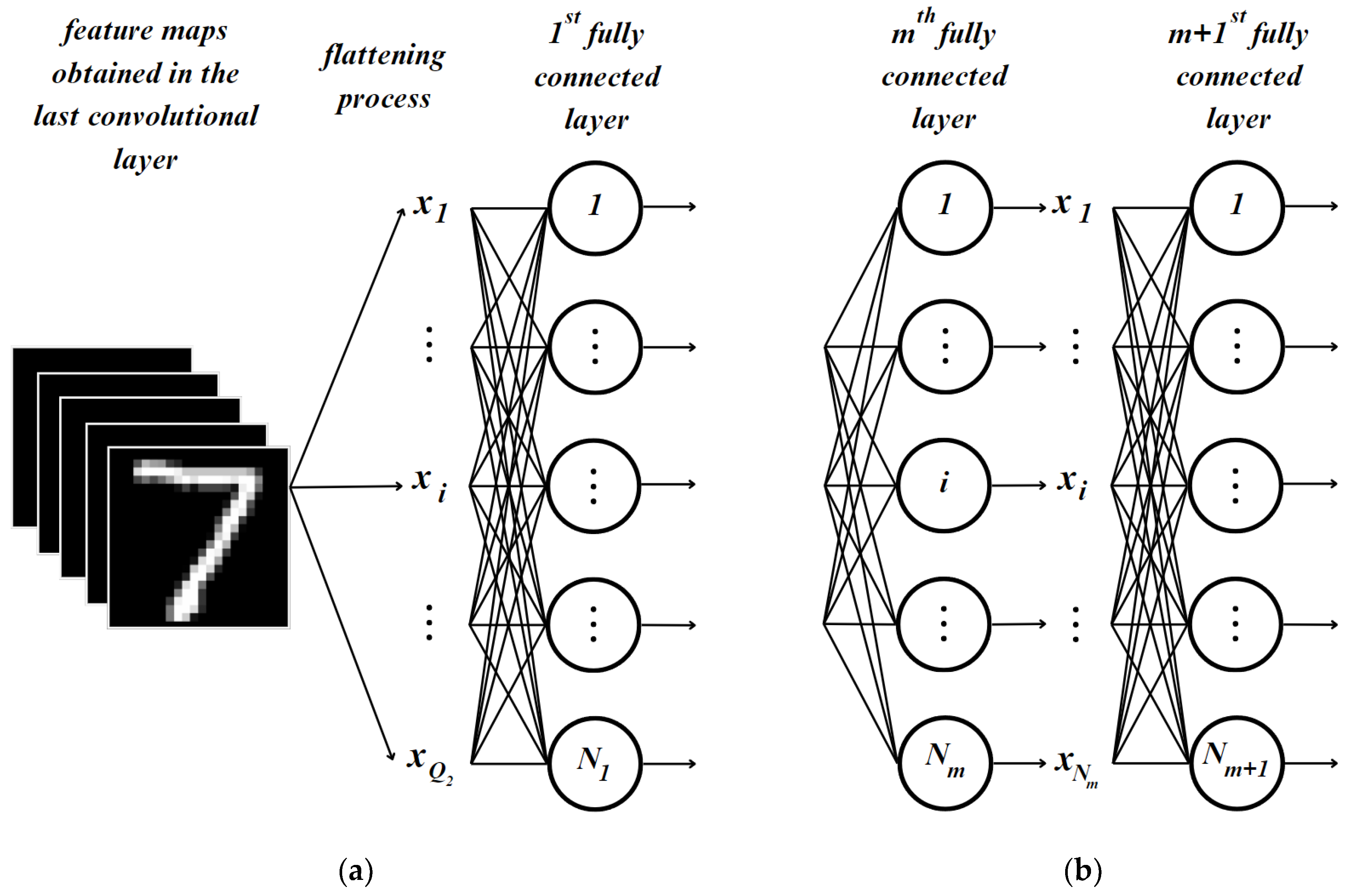
where z n , m + 1 and w i n , m + 1 are the weighted sum and the weights of the n t h neuron of the m + 1 s t layer, respectively ( n = 1 , N m + 1 ¯ , i = 1 , N m ¯ ). According to (10), the error δ i m of the i t h neuron of m t h hidden layer is the dot product of the errors of all neurons in the m + 1 s t layer and the i t h weight of all these neurons. It is essential to note that the i t h weights of all the m + 1 s t layer neurons are responsible for processing the i t h input of these neurons (Figure 1). We would like to slightly modify the error evaluation here to adapt it to this convolutional network. The obtained error should be normalized not by the number of neurons in the preceding ( m + 1 s t ) layer plus one, but by the number of inputs of neurons in the m t h layer. This is because we should share the error among these inputs and then adjust the weights of the neurons that produced them. Hence, we can generalize this approach and say that the error of the i t h neuron in the m t h hidden layer is the dot product of the vector containing the errors of all neurons in the m + 1 s t layer and another vector containing the reciprocal weights responsible for processing the i t h input of these neurons.
Now we can generalize this rule for the first hidden layer and the convolutional layers. According to the considerations presented above, the errors of the first-hidden-layer neurons can be found using (10), but with a changed normalization factor:
δ i 1 = 1 F n = 1 N 2 δ n , 2 w i n , 2 1 ,   i = 1 , N 1 ¯ ,
where F stands for the number of inputs which is equal to the length of flattened feature maps.
The convergence of the learning algorithm based on this error-backpropagation rule for MLMVN is proven in [38]. The convergence of the learning algorithm modified here can be proven in the same manner. If we assume that the algorithm does not converge for some input/output mapping that can be implemented using a network, we will arrive at a contradiction with the latter.

3.2.2. Simple CNNMVN with Two Convolutional Layers

For simplicity, but without loss of generality, let us consider CNNMVN with two convolutional layers, M 1 hidden layers, and one output layer. Any CNNMVN containing more convolutional layers works in the same way. Let the first convolutional layer contain a single kernel and the second one contain H kernels. The m t h hidden layer contains N m neurons ( m = 1 , M 1 ¯ ), and the output layer contains N M neurons. Let an input image be of size ( a 1 × a 1 × 1 ). The kernel size in the first convolutional layer is r 1 × r 1 × 1 ( r 1 < a 1 ). Thus, we obtain a single feature map created by the first convolutional layer, and its size should be equal to a 1 r 1 + 1 × a 1 r 1 + 1 × 1 . Let the kernel size in the second convolutional layer be equal to the size of the feature map obtained in the first convolutional layer r 2 × r 2 × 1 ( r 2 = a 1 r 1 + 1 ). Hence, from the second convolutional layer we obtain H feature maps, each consisting of a single pixel. These feature maps should be flattened into a vector and proceed to the first hidden layer and then to the output layer.
The global and local errors of the output layer should be calculated according to (8) and (9), respectively. The errors of the neurons in the 2 n d , , M 1 s t hidden layers should be found according to (10), and the errors of the first-hidden-layer neurons should be evaluated according to (20). Since each kernel in the feedforward process forms its own feature map and these feature maps are two-dimensional, we should perform feature map flattening before proceeding to the fully connected layer. As a result, we can assume that this flattened vector of outputs is the same as if it was obtained from a layer in the fully connected part (Figure 2). Therefore, to backpropagate the error from the first hidden layer to the last convolutional layer, we should follow the same approach used for error backpropagation to hidden layers in MLMVN. The distinction is that the errors of the corresponding feature map pixels should then be shared among all inputs of the corresponding kernel, and the respective normalization factor should be equal to the size of the kernel. This leads us to the following formula for the last convolutional layer’s errors:
δ h , 2 = 1 Q 2 n = 1 N 1 δ n , 1 w h n , 1 1 ,   S 2 = r 2 r 2 1 ,
where δ h , 2 is the error of the feature map (in this case, a single pixel) produced by the h t h kernel of the second convolutional layer ( h = 1 , H ¯ ); δ n , 1 are the errors of the first hidden layer neurons and w h n , 1 are the neurons’ weights in the first hidden layer that are responsible for processing the h t h input of these neurons; and Q 2 is the normalization factor, which should be equal to the size of the kernel in the second convolutional layer.
To backpropagate the error from the last convolutional layer to the preceding convolutional layers, we should follow the same rule: the error of each pixel of the feature map should be formed from all the weights that process these pixels and the corresponding kernel errors. Before proceeding to these error evaluations, it is important to mention that the image pixels at the corners and edges of an image (or a feature map) and the pixels in the middle of an image (or a feature map) are involved in the respective convolution process a different number of times. For example, a pixel in the top left corner is convolved by the k t h kernel only once, while the next one to the right has already been processed twice (Figure 3).
Let T be the number of times when the i j t h pixel was involved in a convolution. Taking into account all the considerations above, the errors of the feature map pixels created by a single kernel in the first layer are:
δ i j 11 = h = 1 H t = 1 T δ h 2 t w t h 2 1 ,   i , j = a 1 r 1 + 1 ,
where δ i j 11 is the error of the feature map pixel with coordinates i , j produced by a single kernel in the first convolutional layer, and δ h 2 t and w t h 2 are the error of the output and the weight of the h t h kernel in the second convolutional layer that processed i j t h pixel at the t t h convolution, respectively. It is important to note that there is no normalization factor in (22) because there is no further need for error backpropagation.
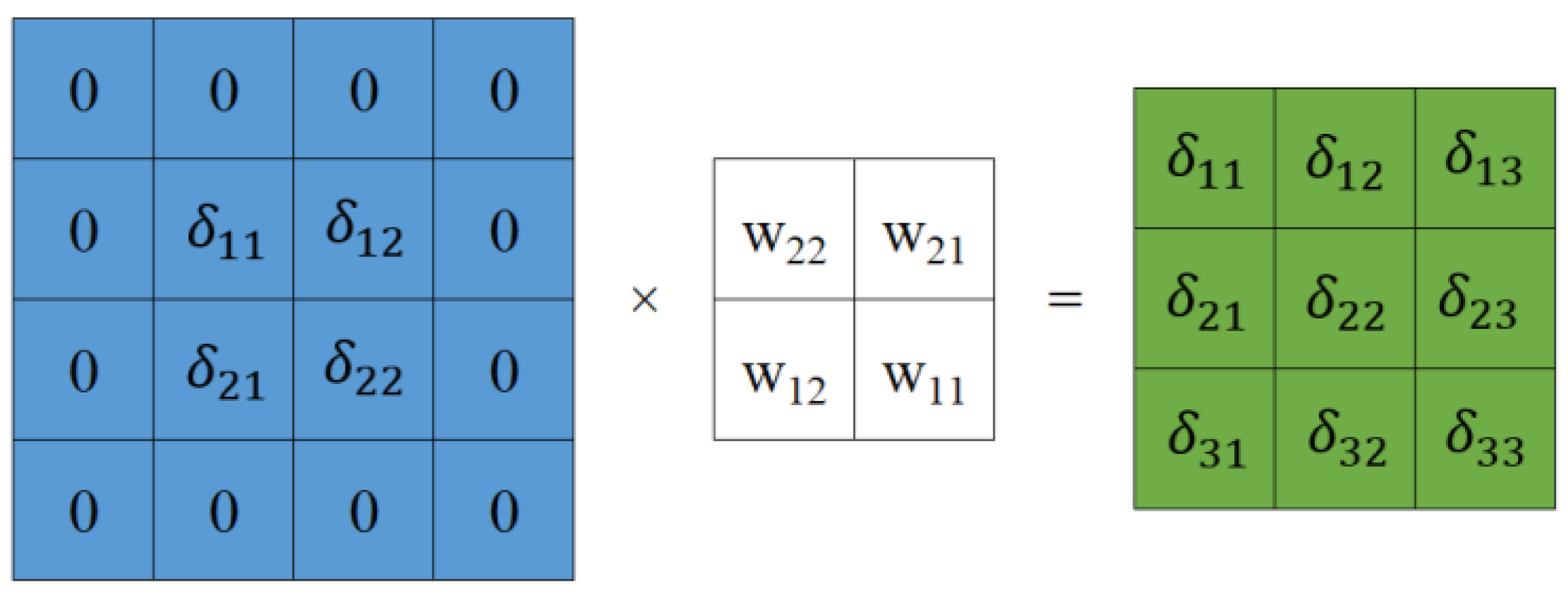
But there is an easier way to backpropagate the errors between convolutional layers: the backward convolution process. This method was proposed for CNNMVN in [62], and it is structurally similar to the error-backpropagation process for real-valued CNNs. To perform backward convolution and backpropagate the errors from the second convolutional layer to the first one, we should add zero padding to the feature map errors of each feature map of the second convolutional layer. Then, we rotate the kernels of the second convolutional layer by 180° and apply convolution to these errors (Figure 4). This process can be represented as follows:
δ i j 11 = h = 1 H u = 1 r 2 v = 1 r 2 δ i + u 1 , j + v 1 h , 2 w r 2 u + 1 , r 2 v + 1 h , 2 1 ,
where w h , 2 is the weight of the h t h kernel in the second convolutional layer and δ h , 2 are the zero padded errors of the feature map obtained by the h t h kernel in the second convolutional layer. The zero padding should be equal to the kernel size minus one, that is r 2 1 . Therefore, a feature map of the errors obtained according to (23) is equivalent to the errors obtained using (22).

3.2.3. CNNMVN: The General Case

Let us now consider CNNMVN containing G convolutional layers, M 1 hidden layers, and one output layer. Let each convolutional layer consist of H g kernels   g = 1 , G ¯ . Let the input image x (or a feature map in the case of convolutional layers from the 2 n d one to the G t h one) be of size a g × b g × d g . Then the kernel size in the g t h convolutional layer is equal to r g × r g × d g ( r p < min a g , b g ). The m t h hidden layer in the fully connected part contains N m neurons ( m = 1 , M 1 ¯ ), and the output layer contains N M neurons.
The errors of all neurons in the fully connected part should be calculated according to (8)–(10) and (20). Then the errors of the neurons in the first hidden layer should be backpropagated to the last-convolutional-layer kernels similarly to how it was done in (21) for a “simple CNNMVN”.
δ i j h G = 1 Q G n = 1 N 1 δ n , 1 w i j h n , 1 1 ,   i = 1 , , a G r G + 1 , j = 1 , , b G r G + 1 , Q G = r G r G c G ,
where δ i j h G is the error of the feature map pixel with coordinates i ,   j , produced by the h t h kernel of the last ( G t h ) convolutional layer, δ n , 1 are the errors of the first hidden layer neurons and w i j h n , 1 are these neurons’ weights that are responsible for processing the i j h t h input, and Q G is the normalization factor which should be equal to the size of the kernel in the last convolutional layer.
To backpropagate the errors from the last convolutional layer to the preceding convolutional layer or in general case from the g t h convolutional layer to the g 1 s t one, we use the same rule as before: the errors of the convolved pixels in the g 1 s t layer depend on the kernel weights that process these pixels and the errors of the neurons (or kernels) in the following layer (which can be the first hidden layer or the next convolutional layer). Let us describe this mathematically. Let T g be the number of times the i j t h pixel was involved into a convolution in the g t h convolutional layer. Then the errors of the kernels in the g 1 s t convolutional layer are
δ i j l , g 1 = 1 Q g 1 h = 1 H g t = 1 T g δ h , g , t w t h , g 1 ,   i = 1 , , a g r g + 1 , j = 1 , , b g r g + 1 , Q g = r g r g c g ,
where δ l , g 1 are the errors of the feature map obtained by the l t h kernel in the g 1 s t convolutional layer ( l = 1 , H g 1 ¯ ); δ h , g , t and w t h , g are the errors of the output and the weights of the h t h kernel in the g t h convolutional layer that process the i j t h pixel in the t t h convolution, respectively; and Q g 1 is a normalization factor which is equal to the size of the kernel in the g 1 t h layer (note that Q 2 = 1 as there is no further error backpropagation from the first convolutional layer).
The same expression for the errors of a respective feature map should also be obtained using the backward convolution. This leads to the following. First, we should zero pad the errors of each feature map in a layer, from which the errors are backpropagated. Then a respective kernel should be rotated by 180°, and then a respective convolution should be performed. It is important to mention that we neither apply zero padding nor flip the depth dimension of a feature map, because a respective kernel does not slide over it in the feedforward process. Thus, we obtain
δ i j l , g 1 = 1 Q g 1 h = 1 H g u = 1 r g v = 1 r g δ i + u 1 , j + v 1 h , g w r g u + 1 , r g v + 1 , l h , g 1 ,
where δ l , g 1 are the errors of the feature map obtained by the l t h kernel in the g 1 s t convolutional layer ( l = 1 , H g 1 ¯ ), δ h , g are the elements of the zero-padded matrix of the errors of the feature map obtained by the h t h kernel in the g t h convolutional layer, w h , g are the weights of the h t h kernel in the g t h convolutional layer, and Q g 1 is a normalization factor which is equal to the size of the kernel in g 1 t h layer (note that Q 2 = 1 as there is no further error backpropagation from the first convolutional layer).
Hence, the CNNMVN error backpropagation for its fully connected part is determined by (8)–(10) and (20), and the error backpropagation for its convolutional part is determined by (24)–(26).
It is also interesting to mention that if the kernels’ size is equal to the input image or feature map size (excluding the neurons’ biases), MLMVN can be considered as a specific subcase of CNNMVN.

3.3. Adjustment of the Weights in CNNMVN

After the error backpropagation is complete, all the weights in both the convolutional and fully connected parts of CNNMVN should be adjusted. To design this process for CNNMVN, we should base it on the respective process of weight adjustment in MLMVN.
A kernel in any convolutional layer basically works similarly to MVN—it calculates a weighted sum of inputs and applies an activation function to it. Hence, to adjust the kernels’ weights, we can employ the same idea as in the error-correction learning rules (6) and (7), which are used to adjust the weights in MVN and MLMVN. However, this idea requires some adaptation. There is one significant distinction between MVN and a kernel in a convolutional layer. An MVN processes one vectorized input at a time and, based on this input, it produces a single output. However, a kernel in any convolutional layer slides over an image (or a feature map), processing multiple inputs and producing multiple outputs accordingly. This means that the error-correction learning rules (6) and (7) for MVN and MLMVN cannot be used directly for CNNMVN. However, in [62], we proposed to employ for kernels’ weight adjustment the same idea of the batch LLS-based learning algorithm [75], which was developed for MLMVN to simultaneously adjust the weights for multiple learning samples belonging to a batch.
Let us have an a × b × d input image and a kernel whose size is r × r × d ( r < min a , b ). Let K be the number of the convolutional windows in an image through which a convolutional kernel is sliding. Thus K = a r + 1 × b r + 1 . Each convolutional window can be flattened and represented as an input vector to a kernel. Then, using a matrix-vector notation, the convolutional operation can be represented as
x 1 x K w 1,1 , 1 w r , r , d = z 1 z K ,
where x i is the flattened input vector ( i = 1 , K ¯ ), w are the kernel weights, and z i are the convolved pixels. According to a batch algorithm and as it was shown in [62], after calculating the errors for all z i , we can represent adjustments, which should be added to the weights to correct them similarly to (11) and obtain the following:
x 1 x K Δ w 1,1 , 1 Δ w r , r , d = δ 1 δ K ,
where Δ w u , v , j are the adjustments terms for kernel weights ( u , v = 1 , r ¯ and j = 1 , d ¯ ) and δ i are the respective errors to be corrected ( i = 1 , K ¯ ). We can rewrite (28) as
X Δ w = δ ,
where X consists of K flattened inputs. This is similar to the MLMVN batch learning described by (11) and (12), where the neural network weights are adjusted simultaneously for multiple learning samples belonging to the same batch. Thus, the system of Equations (28) or (29), which is the same) for unknowns Δ w 1,1 , 1 , , Δ w r , r , d , which is typically overdetermined K r r d , can be solved in a similar way:
Δ w = X δ ,
where X is the Moore–Penrose inversion of X , that is a pseudoinverse matrix of X . Finally, the adjusted weights of the kernel are
W ~ = W + C Δ w ,
where W and W ~ are the weighting vectors before and after correction, “+” is a component-wise addition, and C stands for learning rate. Since the kernel has multiple inputs and outputs, the batch approach allows finding the “best fit” adjustments for all inputs.

3.4. Pooling Layers for CNNMVN

The general purpose of the pooling layer is to reduce the size of a feature map resulting from the processing in a convolutional layer. There are two types of pooling operations for CNNMVN presented in [62]—the “max” pool and the “average” pool.
The “max” pool operation performs downsampling by choosing the maximum value in the corresponding window. Since CNNMVN is a complex-valued neural network, it was considered to utilize the “max” pool operation by comparing the phases of the complex numbers or comparing their magnitudes.
The “average” pool is a downsampling technique that averages the values in the corresponding window. Unlike the “max” pool, this approach is more suitable for CNNMVN since we should not subjectively choose the component of the complex number on which the downsampling is based.
If the pooling layer is applied after the convolutional one, it affects the error-backpropagation process. In the case of “max” pooling, we should calculate only the errors of the pooled pixels, as the other values were dropped and did not participate in further processing. In such a case, Equation (28) should contain only those input vectors whose convolved pixels were pooled. In the case of “average” pooling, we should distribute the error among all the pixels in the corresponding pool window.

4. MLMVN as a Frequency-Domain CNN and the Frequency-Domain Pooling

4.1. MLMVN as a Frequency-Domain CNN

In regular convolutional neural networks, the convolution operation is performed in the spatial domain, but there is another way to perform it—in the frequency domain. According to the Convolution Theorem, the convolution of two signals in the spatial domain is equal to the inverse Fourier transform of the product of their Fourier transforms:
f g = F 1 F G ,
where f and g are two signals or images, F and G are the Fourier transforms of f and g , respectively, the sign is the convolution operator, and the “ ” sign denotes the element-wise multiplication.
It is important to mention that the coefficients of the Fourier transform and the weights of MVN are both complex-valued. Thus, if we employ a Fourier transform of an image as an MLMVN input, it is possible to interpret the weighting of the input as a component-wise multiplication of the Fourier transform of the image with a frequency-domain convolutional kernel (which should in turn be interpreted as a Fourier transform of the respective spatial-domain convolutional kernel). We can therefore associate this operation with the Convolution Theorem. Thus, if the Fourier transform of an image to be classified is used as MLMVN input, all neurons in the first hidden layer of MLMVN can be treated as the convolutional kernels performing a convolution in the frequency domain followed by the processing of its results.
This implies some important distinctions when compared to regular CNNs. The first distinction is that the result of a convolution performed by each neuron in the first hidden layer is not a feature map as in regular CNNs in the spatial domain, but it is a sum of the frequency-domain feature map coefficients, i.e., the sum of the coefficients which should be interpreted as those of the Fourier transform of a respective convolution. Therefore, the second convolutional layer cannot be used in this case. The second distinction is that we cannot set the size of the kernel, and therefore we cannot control the size of the features being extracted. The size of the frequency-domain kernels formed in the first layer is the same as the input image size. However, what is very important in this case is that MLMVN independently determines the features it needs to recognize images. This process becomes self-organized. It is quite interesting to discover what exactly MLMVN needs to extract to recognize images and how it self-organizes this process. We will consider this in Section 5.

4.2. Frequency Domain Pooling

It is obvious that the Fourier transform of any signal (or image, in particular) produces a frequency-domain representation of the same size as the signal. This means that if our input image is of size m × n , its Fourier transform contains m × n Fourier coefficients representing the image in the frequency domain. If these Fourier coefficients are used as inputs to MLMVN, each neuron in the first layer should have ( m × n ) + 1 weights, accordingly. On the one hand, this leads to increased computational costs. On the other hand, not all frequencies are needed to recognize images; only those frequencies that represent important details are essential.
Considering this, it is attractive and important to find a suitable method for downsampling a frequency-domain input to reduce computational complexity and possibly even improve classification capability by eliminating non-essential frequencies. To achieve this, we propose a “frequency pooling” operation as follows.
The frequency representation of a signal or an image contains Fourier coefficients corresponding to the frequencies from which the signal or image is composed. It is also a well-known fact that the higher the frequency, the smaller the details it reproduces, and vice versa. Therefore, based on the size of the objects that should be recognized, we can determine the frequencies important for recognizing these objects and drop the redundant frequencies that are not essential for their recognition.
To perform frequency-domain pooling of an image, we should first apply the Fourier transform (Figure 5a) and perform a circular shift, ensuring that the DC frequency is in the center and the high frequencies are at the edges (Figure 5b). Now the lower frequencies are located at the center, and the higher frequencies are at the corners. To select useful frequencies, we should rely on the Nyquist–Shannon Theorem [76]. It follows from this theorem that the Fourier transform of an image whose size is n × n contains coefficients corresponding to n / 2 2D frequencies. Then, to distinguish any object (or shape) whose size is approximately s × s , we should rely on the frequencies from the 1 s t to the n / 2 s t h   where is the floor function. In such a case, the n / 2 s t h frequency is a cut-off frequency. For example, let us have an image whose size is 32 × 32 . If we need to distinguish an object (or shape) whose size is 4 × 4 , we need to use Fourier coefficients corresponding to the frequencies from the 1 s t one to the 32 / ( 2 × 4 ) = 4 t h one. To distinguish an object (or shape) whose size is 3 × 3 , we need to use Fourier coefficients corresponding to the frequencies from the 1 s t one to the 32 / ( 2 × 3 ) = 6 t h one, etc.
To extract Fourier coefficients corresponding to the selected 2D frequencies, we can use the following rule: a Fourier coefficient with the x ,   y horizontal and vertical indexes should be extracted from the Fourier transform if x 2 + y 2 t , where t is a cut-off frequency. To simplify this process, it is also possible to apply the “diamond” or “zigzag” rule (Figure 5c) to extract selected frequencies around the DC frequency. A few Fourier coefficients may be missing from the extracted ones, but as our experiments show, this does not affect the results while reducing the input size and computational cost. It is important to mention that we do not extract the DC component, as it does not contain information useful for image recognition.

5. Simulation Results and Discussion

To explore the performance of the proposed approaches, we chose to use MNIST [77] and Fashion MNIST [78] datasets. Each of these datasets consists of a training set of 60,000 samples and a test set of 10,000 samples, and each dataset has 10 classes. Each sample is a 28 × 28 grayscale image in the range [0, 255]. It is important to mention that to test the actual recognition capability of both presented approaches, no image preprocessing was performed. All images were taken as they are. For CNNMVN, these images were transformed according to (1), and for MLMVN, as a CNN in the frequency domain, essential frequencies were extracted according to the “diamond” rule described above.
The main goal was to understand how the neural networks learn according to the proposed approaches and define possible ways for improving the learning algorithm. Considering that the learning algorithms for both approaches are based on the heuristic assumption that the error of the network should be equally shared among all the neurons that participated in its formation, we made some changes to the learning process. In the next two sections, these changes are considered, and the corresponding experimental results are given.

5.1. Custom Normalization for CNNMVN and Experiments

The experimental results in [62,63] demonstrated the high performance and potential of CNNMVN. On the one hand, it shows a high accuracy rate, but on the other hand, to achieve this, we should use custom normalization for the error-backpropagation and weight adjustment processes. According to the error-backpropagation algorithm described above, the errors of the fully connected layers should be calculated using (8)–(10) and (20), and the errors of the convolutional layers according to (24) and (25). All these formulas have a normalization factor equal to the number of inputs to the layer, regardless of whether it is a convolutional layer or a fully connected one.
The analysis of the error backpropagation process showed that the errors decrease at each layer, starting from the output layer. This leads to the conclusion that the neuron weights are also adjusted less starting from the output layer and moving back to the convolutional layers. This is especially noticeable in (20), where the error is backpropagated from the second hidden layer to the first one, and the normalization factor is equal to the size of the flattened feature maps, which is large in most cases.
Thus, we decided to adjust the normalization factors for the CNNMVN learning algorithm. First, we decided to remove the normalization factors in (6), where the neurons in the fully connected layer are adjusted. Second, we removed the normalization factor in (20) when the error is backpropagated from the second hidden layer to the first one. Third, we added self-adapting normalization for the convolutional layers. Hence, the error of each convolved pixel is additionally normalized by the absolute value of the current weighted sum resulting in this pixel. Now, the feature map errors of the last convolutional layer (24) with additional normalization can be found as follows:
δ i j h G = 1 Q G c i j h , G n = 1 N 1 δ n , 1 w i j h n , 1 1 ,   i = 1 , , a g r g + 1 , j = 1 , , b g r g + 1 , Q G = r G r G c G ,
and the errors of the feature maps in preceding convolutional layers (25) with additional normalization factor are
δ i j l , g 1 = 1 Q g 1 c i j h , g 1 h = 1 H g t = 1 T g δ h , g , t w t h , g 1 ,   i = 1 , , a g r g + 1 , j = 1 , , b g r g + 1 , Q g = r g r g c g ,
where c i j h , g is the absolute value of the convolved pixel with coordinates i , j in the h t h kernel in the g t h convolutional layer ( h = 1 , H g ¯ , g = 2 , G ¯ ) obtained by (17).
The adjusted normalization was tested using “one sample” learning and a single hidden fully connected layer. Each kernel in the convolutional layer had a stride of 1, and the pool stride (if a pooling layer was used) was 2. We also used the modified soft margins algorithm [74], which skips the learning samples if the sample’s errors are less than a predefined soft margins threshold, which was equal to π / 18 . The learning lasted 20 epochs.
Experimental results for the MNIST dataset are presented in Table 1, and for the Fashion MNIST dataset in Table 2. The notation is as follows: for example, in topology 16C5-P2-h128-o10, parameter 16C5 means a convolutional layer with 16 kernels and a kernel size of 5 × 5; P2 stands for the pooling layer with a window size of 2 × 2; h128 is the number of neurons in a single hidden layer in the fully connected part of the network; and o10 stands for the number of output neurons. Each of output neurons performs binary classification using the “One vs. All” approach. The “winner” neuron is determined by the closeness of its weighted sum to the desired output of that neuron.
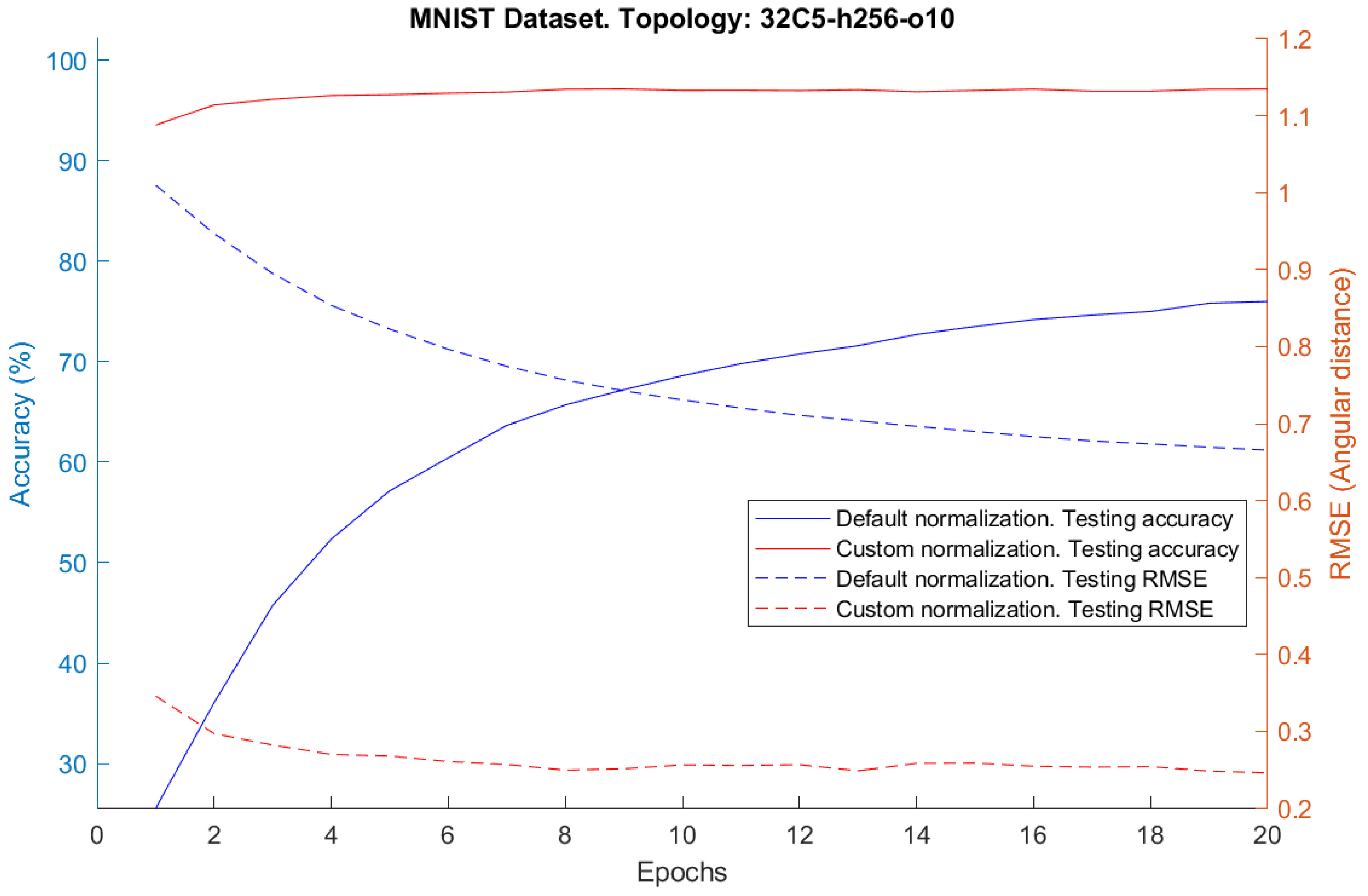
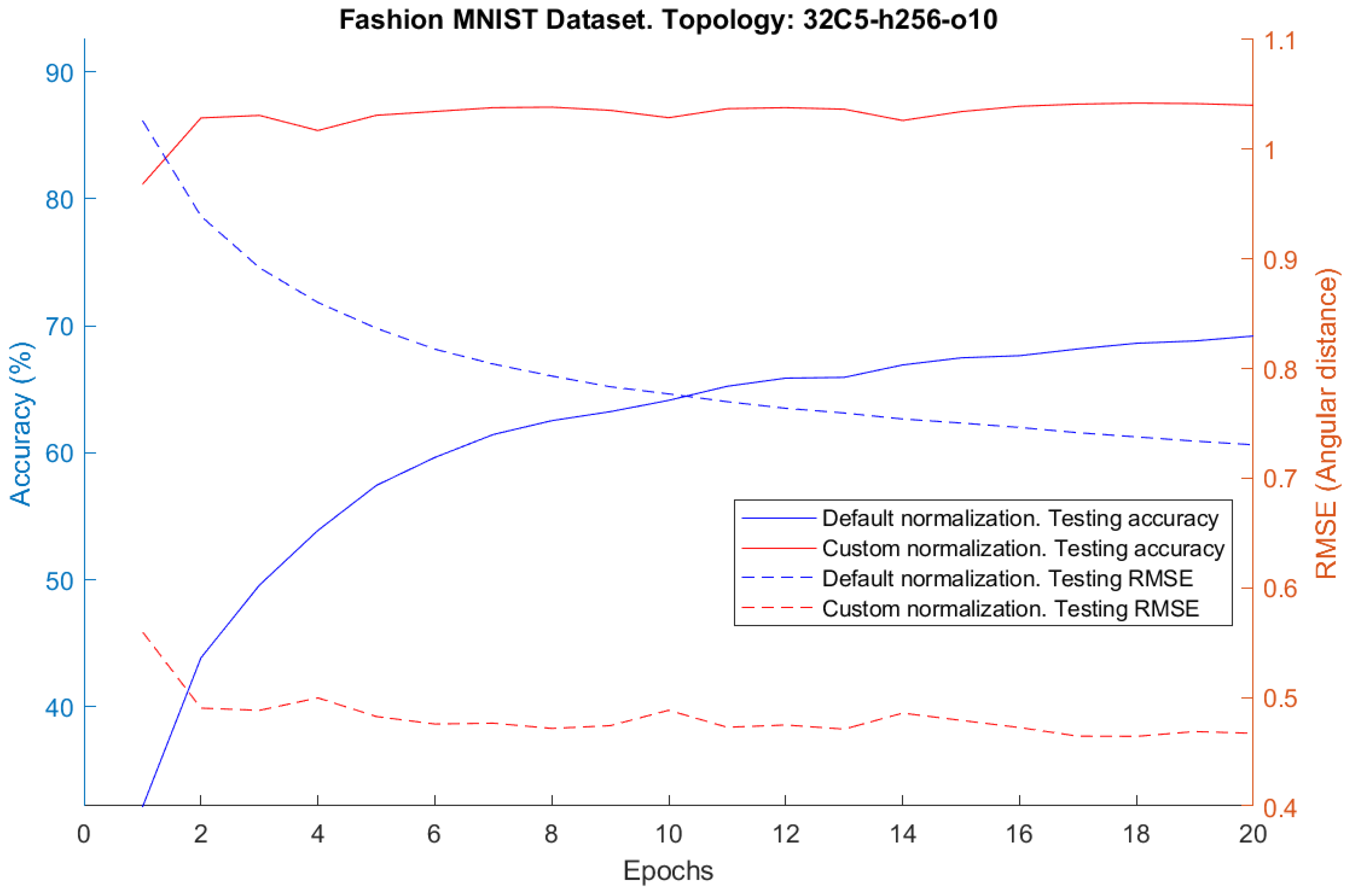
Another observation is that the network continues long-term learning without overfitting and maintains stable recognition accuracy with the custom normalization approach (Figure 6 and Figure 7). It is also evident that CNNMVN with default normalization learns much more slowly and is unable to achieve the same accuracy as the model with custom normalization. The experiments have also shown that both pooling approaches (“max” and “average”) lower the classification accuracy. This is quite obvious due to the loss of information. Also, it is still an open question how to perform pooling efficiently for complex-valued data and define the most valuable data. We also checked the recommendation provided in [53], to use max pooling over magnitudes of the respective complex numbers.
However, while it worked better for the complex-valued hyperbolic tangent activation function in [53], it did not show improvements in conjunction with the MVN activation function (4) in our experiments. Thus, pooling in the complex domain still remains an open problem and should be a subject for future work.

5.2. MLMVN as a CNN in the Frequency Domain

To evaluate the capability of this approach, we used two topologies: with one and two hidden layers. In both cases, the first hidden layer was considered convolutional. Therefore, the topology was either I → H1 → O or I → H1 → H2 → O, where I stands for the neural network’s input, H1 and H2 represent the number of neurons in the first and second hidden layer, respectively, and O denotes the number of neurons in the output layer. In both cases, the output layer consisted of 10 neurons, each performing binary classification using the “One vs. All” approach. The “winner” neuron is determined by the closeness of its weighted sum to the desired output of that neuron, the same rule as was used in CNNMVN.
The inputs to the network were the normalized Fourier coefficients of the normalized input images (their range was transformed to [0, 1]) obtained using frequency pooling. For the MNIST images, we generated three datasets with frequencies 1–5, 1–6, and 1–7, and for the Fashion MNIST images, we have chosen frequencies 1–7, 1–8, and 1–9.
In general, the entire learning process in this approach is equivalent to regular MLMVN, except that the inputs are the Fourier coefficients of the respective frequencies. However, we also incorporated some improvements. The first improvement is the use of error correction for neuron weights using the self-adaptive learning rule (7). The second improvement is that we calculated the global error of the network (5) as the difference between the desired output and the actual weighted sum, which is equivalent to not using the activation function in the output layer. This approach was first introduced in [74] and allows for improved generalization capability in regular MLMVN. Therefore, the global error of the network is given by:
δ * = D z ,
where δ * is the global error, D is the desired output of the neuron, and z is the actual weighted sum of the output neuron.
For our tests, we also applied the batch learning algorithm technique with a batch size of 20,000 samples. At each step, the neural network learned samples from the batch and then moved on to the next batch until all elements of the training dataset were used. A new epoch then started, and these steps were repeated. Additionally, we employed the soft margins technique with a threshold of π/12. The learning process continued for 200 epochs.
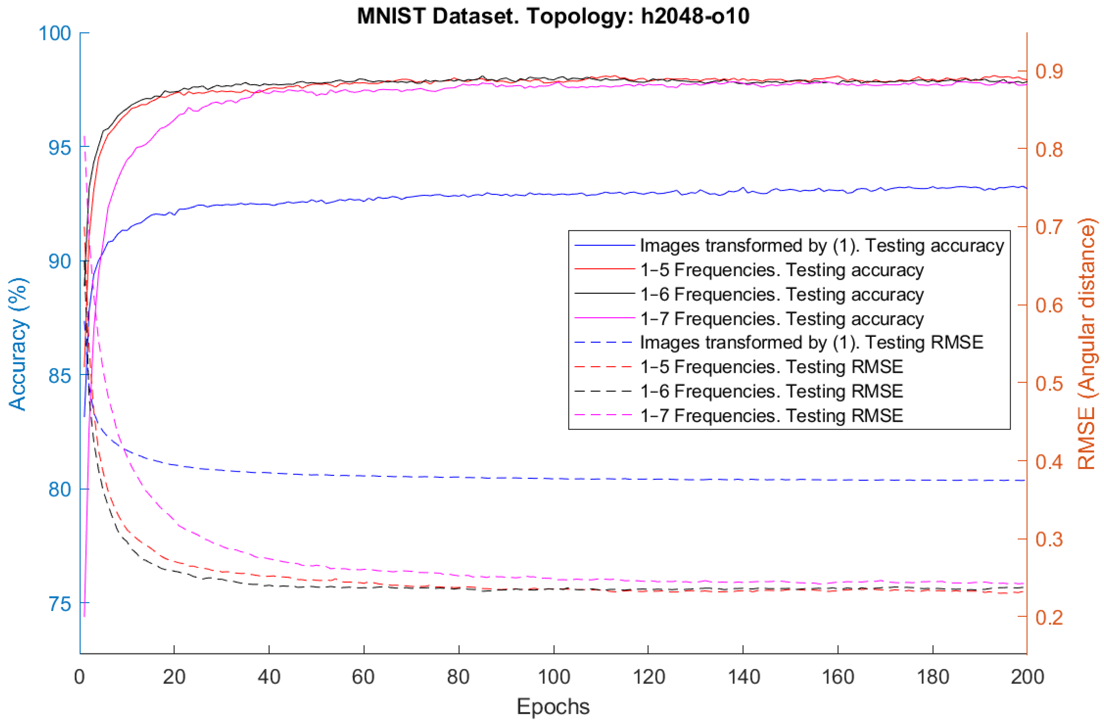
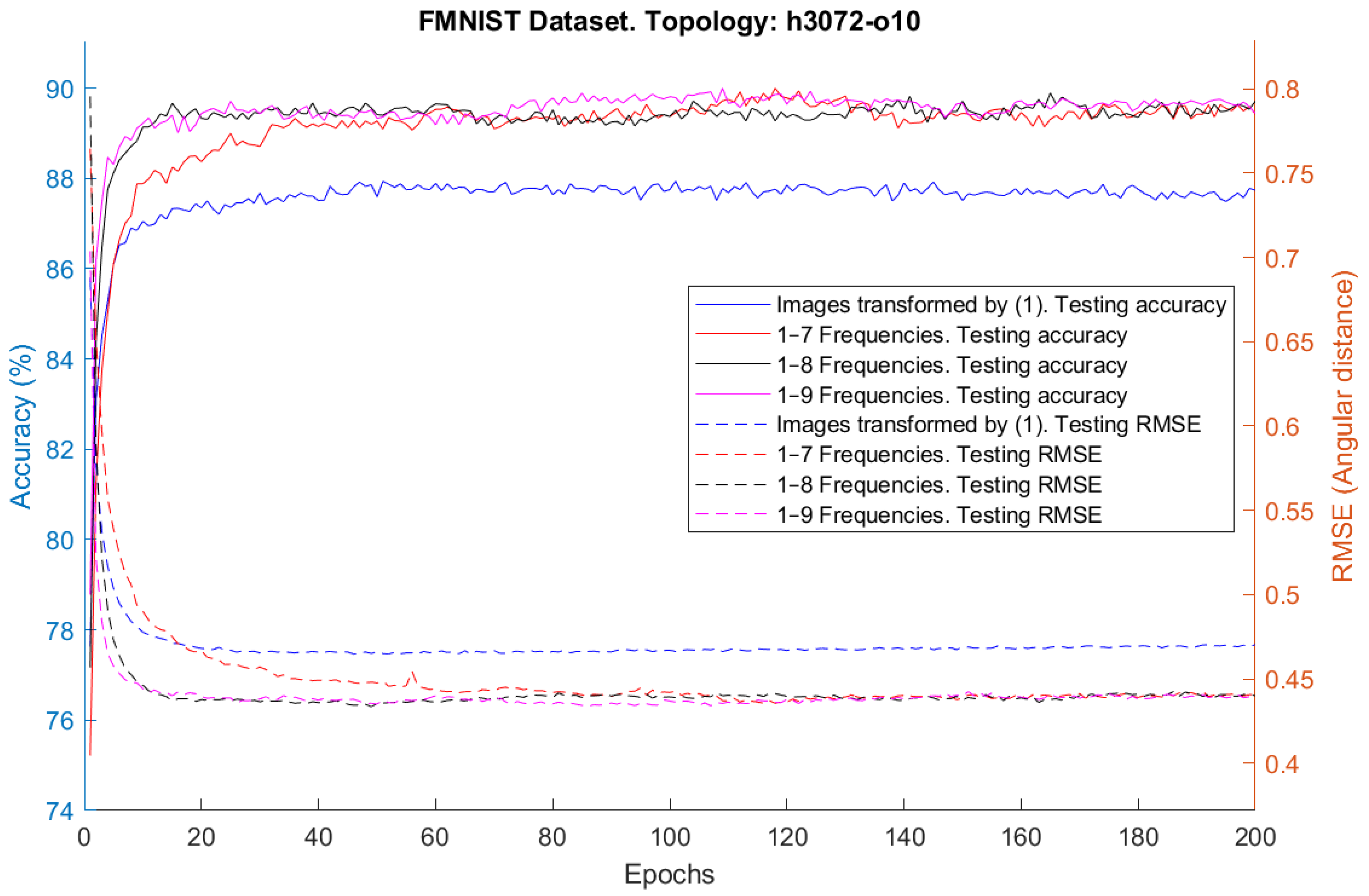
The experimental results for the MNIST dataset are presented in Table 3, and for the Fashion MNIST dataset in Table 4. They demonstrate the high potential of MLMVN as a CNN in the frequency domain and warrant further examination. Our attention was drawn to the fact that all results are nearly the same across different topologies and the number of frequencies used. It is evident that in most cases, the larger the network, the faster it reaches its peak accuracy, after which further learning becomes redundant. It was established that the reason is similar to that for CNNMVN: the network’s errors decrease during the training process, and the normalization factors in the error-backpropagation process drive these errors towards zero, resulting in minimal changes in neuron weights and a slowdown in learning. Like CNNMVN, this network demonstrates the capability to learn over many epochs without overfitting. Figure 8 and Figure 9 illustrate the stable accuracy rate of the testing dataset during the training process.
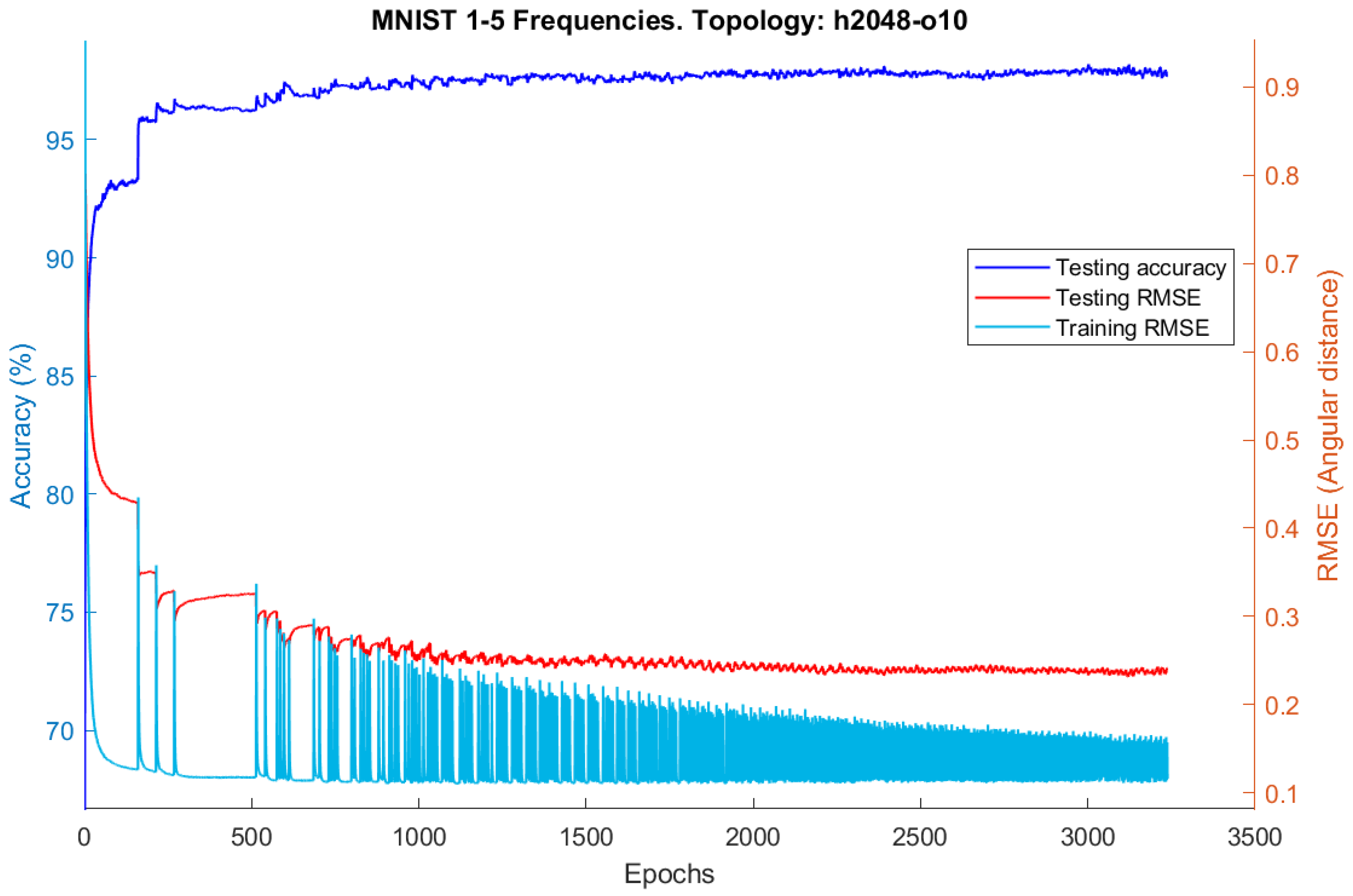
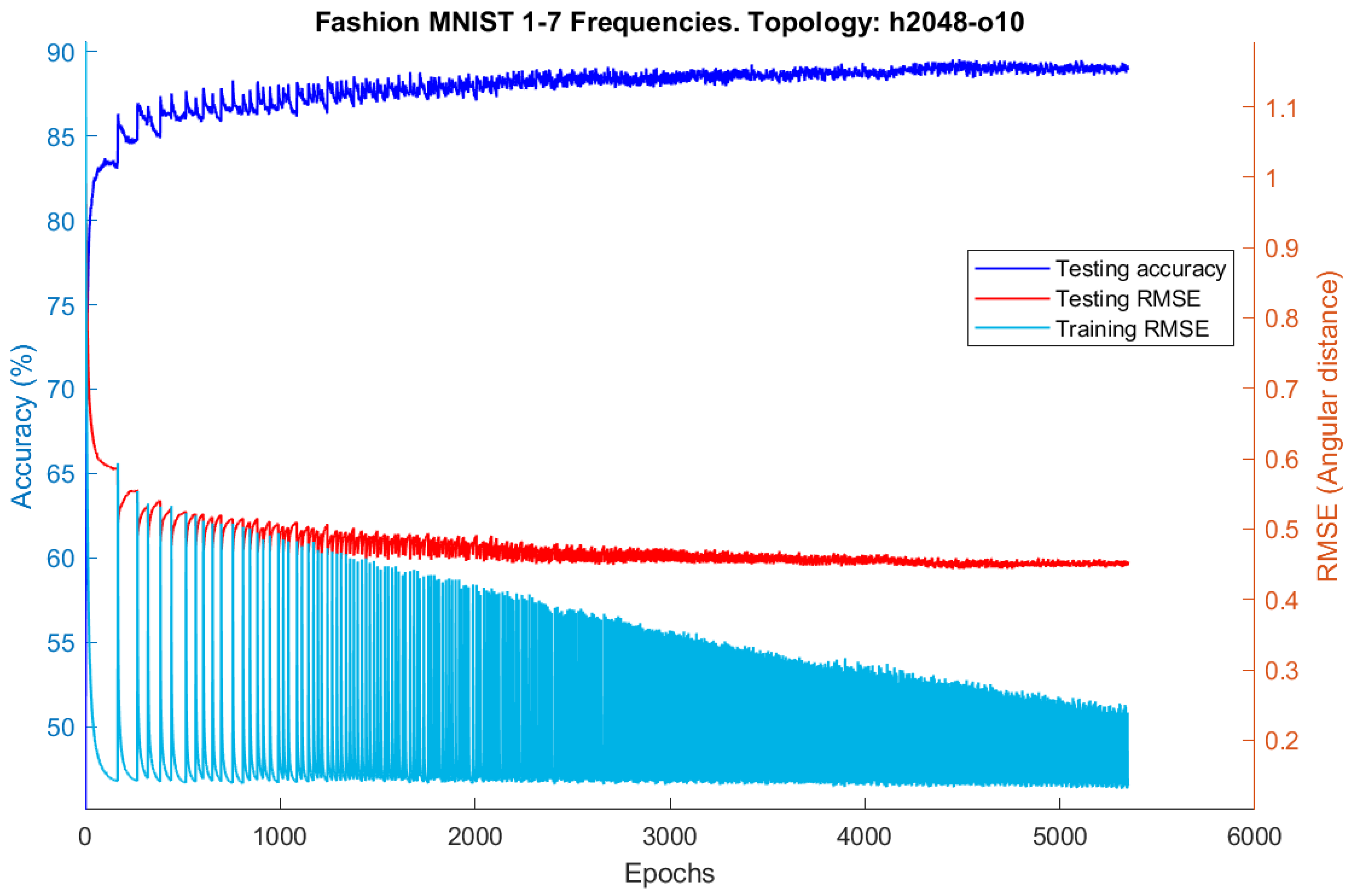
We also conducted another type of testing: strict batch learning. Unlike the first type, here the neural network learns samples from the batch at each step but proceeds to the next batch only after learning all the samples from the current one with the zero learning error—if any samples in the batch produce the error, the same batch is repeated in the next learning step. The batch size was 10,000, and the learning lasted for 100 epochs. Other hyperparameters and normalizations were kept the same as in the first type of testing. This approach yielded results similar to the ones with the default batch learning, but it required significantly more iterations and computational time to complete all epochs. The experimental results are presented in Table 5.
Figure 10 and Figure 11 display the accuracy and RMSE drop for training and testing datasets during the learning process. The spikes we observe correspond to the start of a new iteration with a new batch.

5.3. Comparative Analysis of Convolved Images Produced by CNNMVN and MLMVN as a CNN in the Frequency Domain

It is interesting to analyze the convolutions performed by CNNMVN in the spatial domain and by MLMVN in the frequency domain. In both networks, these convolutions result from the learning process. By analyzing these convolutions, we can see which details they extract from images to recognize them.
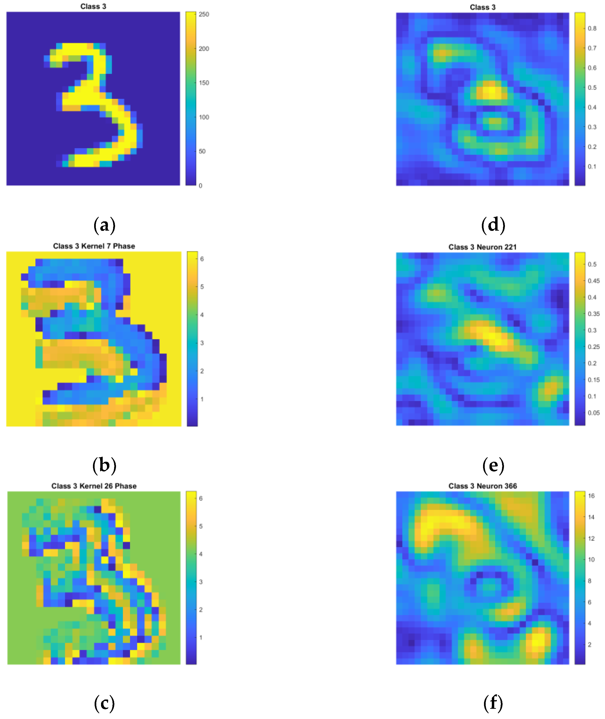
While both networks perform convolutions, these convolutions appear to be quite different from each other. This is illustrated in Figure 12 using one image from the MNIST dataset (class “3”—Figure 12a). CNNMVN creates convolutional kernels that perform high-pass (Figure 12c) and medium-pass filtering (Figure 12b). The latter can be compared to unsharp masking, well known in image processing as a family of filters that distinguish image details. This can clearly be seen from the feature maps resulting from the respective convolutions. We may also conclude that these convolutions are quite similar to the ones performed by kernels in the first convolutional layer of a traditional CNN. MLMVN performs convolution in the frequency domain. Figure 12d depicts an image resulting from frequency-domain downsampling. It was obtained by applying the inverse Fourier transform to the Fourier spectrum of an image where only Fourier coefficients corresponding to frequencies 1–5 were preserved. By taking the inverse Fourier transform from any component-wise product of the downsampled Fourier transform (of an image shown in Figure 12d used as a network input) and a weighting vector, we can obtain a respective convolved image. As this image is complex-valued in general, we extract its magnitude to visualize it. Two of such images are presented in Figure 12e,f. Analyzing these convolved images, we may conclude that frequency-domain convolutions resulting from the learning process likely extract structural components from images, breaking them down into respective structures. Each convolutional kernel in the frequency domain resulting from the learning process becomes responsible for extracting structural elements that appear to be useful for recognition due to the network’s self-organization based on its learning process. It is also possible to conclude that these convolutions are similar to the ones extracting high-level features in traditional CNNs and performed in the second and further convolutional layers (if any).

5.4. Comparison of the Capabilities of CNNMVN and MLMVN as a Frequency-Domain CNN with Those of Other Networks

As mentioned above, our goal was to test the “pure” image recognition capabilities of both networks used in this paper. Thus, we intentionally did not apply any kind of preprocessing to the images used for learning and testing. Additionally, in all our experiments, we intentionally used the simplest possible network topologies to test the “pure” image recognition capabilities of both networks.
Several researchers have published works reporting formally better recognition rates for the same two image datasets used here. However, these results were obtained after various kinds of preprocessing were applied to the images and using networks with more complicated topologies (more convolutional layers, more kernels, and more hidden layers in the fully connected part of a respective CNN). For example, the best result for the MNIST dataset (99.87%) was reported in [78], but an incomparably more complicated network was used (an ensemble of three CNNs with 3 × 3, 5 × 5, and 7 × 7 convolutional kernels) in conjunction with sophisticated data preprocessing (data augmentation consisting of rotation and translation). Data augmentation, training data expansion, and elastic distortions [79] are typical preprocessing methods that improve results. We intentionally did not use these methods as our goal was to test the network’s generalization and recognition capabilities as they are. To obtain a higher classification rate using a regular real-valued CNN without data preprocessing, a larger network with some more sophisticated learning techniques (like dropout and various kinds of optimization) should be used. This is shown, for example, in [80], where to reach 98.96% classification accuracy on the MNIST dataset, a CNN with two convolutional layers containing 64 kernels each along with modified learning algorithm has been used.
We also want to mention the result reported for the MNIST dataset in [81] (98.4% recognition accuracy). Our results obtained using MLMVN as a frequency-domain CNN are comparable. A regular MLP with a single hidden layer containing 800 neurons was used in [81], and we employed MLMVN with a single hidden layer with various numbers of neurons there. However, an entire 28 × 28 image was used as a network input in [81] (that is, 784 inputs were used), while we used Fourier coefficients corresponding to the first five to seven frequencies as an input. That is, we employed between 60 inputs (five frequencies) and 112 inputs (seven frequencies)—fewer inputs than in [81] by an order of magnitude.
Our results for the Fashion MNIST dataset are also comparable to the results reported by other authors. In [80], 89.65% accuracy is reported for an ordinal feedforward network, but with an optimizer. A CNN with two convolutional layers containing 64 kernels each along with modified learning algorithm makes it possible to reach 92.76% accuracy [80]. To obtain better results, a CNN with multiple convolutional layers and/or data preprocessing should be used [80,82]. The use of hierarchical CNNs [34] (that is, the use of a significantly more sophisticated technique) may also boost classification accuracy for the Fashion MNIST dataset [82].
Hence, we may conclude that our simulation results are comparable to those obtained by other authors. Moreover, our approach has potential that is yet to be discovered—if more sophisticated network topologies, various kinds of preprocessing, and adaptive modified learning techniques are used.

6. Conclusions and Future Work

Thus, in this paper, we considered image recognition employing a complex-valued convolutional neural network with multi-valued neurons (CNNMVN) as a spatial-domain convolutional neural network and a multilayer neural network with multi-valued neurons (MLMVN) as a frequency-domain convolutional neural network.
We derived the error-backpropagation rule for CNNMVN. We considered in detail how a frequency-domain convolution can be utilized using MLMVN and suggested using frequency-domain downsampling as an analogue of pooling in the spatial domain.
It was shown that both neural networks can be used for image recognition. Their capabilities were tested using two classical image datasets—MNIST and Fashion MNIST. Our intention was to test both networks using images as they are, without any kind of preprocessing. This allowed us to examine the actual recognition capability of both presented approaches.
Future work will focus on further investigation of the custom normalization for CNNMVN and the investigation of networks with multiple convolutional layers. Additionally, both approaches should be tested on other popular datasets such as CIFAR-10 and CIFAR-100. It would also be interesting to test how preprocessing data techniques may improve the network’s generalization capabilities and recognition rate.

Author Contributions

Conceptualization, I.A.; methodology, I.A. and A.V.; software, A.V.; validation, I.A. and A.V.; formal analysis, I.A. and A.V.; investigation, I.A. and A.V.; data curation, I.A. and A.V.; writing—original draft preparation, A.V.; writing—review and editing, I.A. and A.V.; visualization, A.V. All authors have read and agreed to the published version of the manuscript.

Funding

This research received no external funding.

Data Availability Statement

Data and software used in the simulation experiments should be shared through the links provided in the final version of the paper submitted for publication.

Acknowledgments

Most of the computational experiments were performed using the facilities of the Kakos Center for Scientific Computing at Kakos School of Arts and Science, Manhattan College, Riverdale, NY, USA.

Conflicts of Interest

The authors declare no conflicts of interest.

References

  1. Krizhevsky, A.; Sutskever, I.; Hinton, G.E. ImageNet Classification with Deep Convolutional Neural Networks. In Proceedings of the Advances in Neural Information Processing Systems, Lake Tahoe, NV, USA, 3–6 December 2012; Curran Associates, Inc.: Red Hook, NY, USA, 2013; Volume 25. [Google Scholar]
  2. LeCun, Y.; Huang, F.J.; Bottou, L. Learning Methods for Generic Object Recognition with Invariance to Pose and Lighting. In Proceedings of the 2004 IEEE Computer Society Conference on Computer Vision and Pattern Recognition, CVPR 2004, Washington, DC, USA, 27 June–2 July 2004; IEEE: Washington, DC, USA, 2004; Volume 2, pp. 97–104. [Google Scholar]
  3. Jarrett, K.; Kavukcuoglu, K.; Ranzato, M.A.; LeCun, Y. What Is the Best Multi-Stage Architecture for Object Recognition? In Proceedings of the 2009 IEEE 12th International Conference on Computer Vision, Kyoto, Japan, 27 September–4 October 2009; IEEE: Kyoto, Japan, 2009; pp. 2146–2153. [Google Scholar]
  4. Gifford, N.; Ahmad, R.; Soriano Morales, M. Text Recognition and Machine Learning: For Impaired Robots and Humans. Alta. Acad. Rev. 2019, 2, 31–32. [Google Scholar] [CrossRef]
  5. Wu, D.; Zhang, J.; Zhao, Q. A Text Emotion Analysis Method Using the Dual-Channel Convolution Neural Network in Social Networks. Math. Probl. Eng. 2020, 2020, 6182876. [Google Scholar] [CrossRef]
  6. Kaur, P.; Garg, R. Towards Convolution Neural Networks (CNNs): A Brief Overview of AI and Deep Learning. In Inventive Communication and Computational Technologies; Ranganathan, G., Chen, J., Rocha, Á., Eds.; Lecture Notes in Networks and Systems; Springer: Singapore, 2020; Volume 89, pp. 399–407. ISBN 9789811501456. [Google Scholar]
  7. Lin, W.; Ding, Y.; Wei, H.-L.; Pan, X.; Zhang, Y. LdsConv: Learned Depthwise Separable Convolutions by Group Pruning. Sensors 2020, 20, 4349. [Google Scholar] [CrossRef]
  8. Wang, A.; Wang, M.; Jiang, K.; Cao, M.; Iwahori, Y. A Dual Neural Architecture Combined SqueezeNet with OctConv for LiDAR Data Classification. Sensors 2019, 19, 4927. [Google Scholar] [CrossRef] [PubMed]
  9. Zhao, Y.; Lu, J.; Chen, X. An Accelerator Design Using a MTCA Decomposition Algorithm for CNNs. Sensors 2020, 20, 5558. [Google Scholar] [CrossRef]
  10. Caldeira, M.; Martins, P.; Cecílio, J.; Furtado, P. Comparison Study on Convolution Neural Networks (CNNs) vs. Human Visual System (HVS). In Beyond Databases, Architectures and Structures. Paving the Road to Smart Data Processing and Analysis; Kozielski, S., Mrozek, D., Kasprowski, P., Małysiak-Mrozek, B., Kostrzewa, D., Eds.; Communications in Computer and Information Science; Springer International Publishing: Cham, Switzerland, 2019; Volume 1018, pp. 111–125. ISBN 978-3-030-19092-7. [Google Scholar]
  11. Yar, H.; Abbas, N.; Sadad, T.; Iqbal, S. Lung Nodule Detection and Classification Using 2D and 3D Convolution Neural Networks (CNNs). In Artificial Intelligence and Internet of Things; CRC Press: Boca Raton, FL, USA, 2021; pp. 365–386. ISBN 978-1-00-309720-4. [Google Scholar]
  12. Gad, A.F. Convolutional Neural Networks. In Practical Computer Vision Applications Using Deep Learning with CNNs; Apress: Berkeley, CA, USA, 2018; pp. 183–227. ISBN 978-1-4842-4166-0. [Google Scholar]
  13. Beysolow Ii, T. Convolutional Neural Networks (CNNs). In Introduction to Deep Learning Using R.; Apress: Berkeley, CA, USA, 2017; pp. 101–112. ISBN 978-1-4842-2733-6. [Google Scholar]
  14. Lin, L.; Liang, L.; Jin, L.; Chen, W. Attribute-Aware Convolutional Neural Networks for Facial Beauty Prediction. In Proceedings of the Twenty-Eighth International Joint Conference on Artificial Intelligence, Macao, China, 10–16 August 2019; International Joint Conferences on Artificial Intelligence Organization: Macao, China, 2019; pp. 847–853. [Google Scholar]
  15. Hua, J.; Gong, X. A Normalized Convolutional Neural Network for Guided Sparse Depth Upsampling. In Proceedings of the Twenty-Seventh International Joint Conference on Artificial Intelligence, Stockholm, Sweden, 13–19 July 2018; International Joint Conferences on Artificial Intelligence Organization: Stockholm, Sweden, 2018; pp. 2283–2290. [Google Scholar]
  16. Singh, P.; Namboodiri, V.P. SkipConv: Skip Convolution for Computationally Efficient Deep CNNs. In Proceedings of the 2020 International Joint Conference on Neural Networks (IJCNN), Glasgow, UK, 19–24 July 2020; IEEE: Glasgow, UK, 2020; pp. 1–8. [Google Scholar]
  17. Magalhães, D.; Pozo, A.; Santana, R. An Empirical Comparison of Distance/Similarity Measures for Natural Language Processing. In Proceedings of the Anais do XVI Encontro Nacional de Inteligência Artificial e Computacional (ENIAC 2019), Salvador, Brazil, 15–18 October 2019; Sociedade Brasileira de Computação—SBC: Porto Alegre, RS, Brazil, 2019; pp. 717–728. [Google Scholar]
  18. Xiao, X.; Qiang, Y.; Zhao, J.; Zhao, P. A Deep Learning Model of Automatic Detection of Pulmonary Nodules Based on Convolution Neural Networks (CNNs). In Bio-Inspired Computing—Theories and Applications; Gong, M., Pan, L., Song, T., Zhang, G., Eds.; Communications in Computer and Information Science; Springer: Singapore, 2016; Volume 681, pp. 349–361. ISBN 978-981-10-3610-1. [Google Scholar]
  19. Venkatesan, R.; Li, B. Modern and Novel Usages of CNNs. In Convolutional Neural Networks in Visual Computing; CRC Press: Boca Raton, FL, USA; Taylor & Francis: London, UK, 2017; pp. 117–146. ISBN 978-1-315-15428-2. [Google Scholar]
  20. Sirish Kaushik, V.; Nayyar, A.; Kataria, G.; Jain, R. Pneumonia Detection Using Convolutional Neural Networks (CNNs). In Proceedings of First International Conference on Computing, Communications, and Cyber-Security (IC4S 2019); Singh, P.K., Pawłowski, W., Tanwar, S., Kumar, N., Rodrigues, J.J.P.C., Obaidat, M.S., Eds.; Lecture Notes in Networks and Systems; Springer: Singapore, 2020; Volume 121, pp. 471–483. ISBN 9789811533686. [Google Scholar]
  21. Rath, M.; Reddy, P.S.D.; Singh, S.K. Deep Convolutional Neural Networks (CNNs) to Detect Abnormality in Musculoskeletal Radiographs. In Second International Conference on Image Processing and Capsule Networks; Chen, J.I.-Z., Tavares, J.M.R.S., Iliyasu, A.M., Du, K.-L., Eds.; Lecture Notes in Networks and Systems; Springer International Publishing: Cham, Switzerland, 2022; Volume 300, pp. 107–117. ISBN 978-3-030-84759-3. [Google Scholar]
  22. Wang, Z.; Lan, Q.; He, H.; Zhang, C. Winograd Algorithm for 3D Convolution Neural Networks. In Artificial Neural Networks and Machine Learning—ICANN 2017; Lintas, A., Rovetta, S., Verschure, P.F.M.J., Villa, A.E.P., Eds.; Lecture Notes in Computer Science; Springer International Publishing: Cham, Switzerland, 2017; Volume 10614, pp. 609–616. ISBN 978-3-319-68611-0. [Google Scholar]
  23. Xiao, L.; Zhang, H.; Chen, W.; Wang, Y.; Jin, Y. Transformable Convolutional Neural Network for Text Classification. In Proceedings of the Twenty-Seventh International Joint Conference on Artificial Intelligence, Stockholm, Sweden, 13–19 July 2018; International Joint Conferences on Artificial Intelligence Organization: Stockholm, Sweden, 2018; pp. 4496–4502. [Google Scholar]
  24. Xie, C.; Li, C.; Zhang, B.; Chen, C.; Han, J.; Liu, J. Memory Attention Networks for Skeleton-Based Action Recognition. In Proceedings of the Twenty-Seventh International Joint Conference on Artificial Intelligence, Stockholm, Sweden, 13–19 July 2018; International Joint Conferences on Artificial Intelligence Organization: Stockholm, Sweden, 2018; pp. 1639–1645. [Google Scholar]
  25. Xu, J.; Zhang, X.; Li, W.; Liu, X.; Han, J. Joint Multi-View 2D Convolutional Neural Networks for 3D Object Classification. In Proceedings of the Twenty-Ninth International Joint Conference on Artificial Intelligence, Yokohama, Japan, 11–17 July 2020; International Joint Conferences on Artificial Intelligence Organization: Yokohama, Japan, 2020; pp. 3202–3208. [Google Scholar]
  26. Toledo, Y.; Almeida, T.D.; Bernardini, F.; Andrade, E. A Case of Study about Overfitting in Multiclass Classifiers Using Convolutional Neural Networks. In Proceedings of the Anais do XVI Encontro Nacional de Inteligência Artificial e Computacional (ENIAC 2019), Salvador, Brazil, 15–18 October 2019; Sociedade Brasileira de Computaçã—SBC: Porto Alegre, RS, Brazil; pp. 799–810. [Google Scholar]
  27. Zeng, L.; Wang, Z.; Tian, X. KCNN: Kernel-Wise Quantization to Remarkably Decrease Multiplications in Convolutional Neural Network. In Proceedings of the Twenty-Eighth International Joint Conference on Artificial Intelligence, Macao, China, 10–16 August 2019; International Joint Conferences on Artificial Intelligence Organization: Macao, China, 2019; pp. 4234–4242. [Google Scholar]
  28. Nikzad, M.; Gao, Y.; Zhou, J. Attention-Based Pyramid Dilated Lattice Network for Blind Image Denoising. In Proceedings of the Thirtieth International Joint Conference on Artificial Intelligence, Montreal, QC, Canada, 19–27 August 2021; International Joint Conferences on Artificial Intelligence Organization: Montreal, QC, Canada, 2021; pp. 931–937. [Google Scholar]
  29. Yin, W.; Schütze, H. Attentive Convolution: Equipping CNNs with RNN-Style Attention Mechanisms. Trans. Assoc. Comput. Linguist. 2018, 6, 687–702. [Google Scholar] [CrossRef]
  30. Park, S.-S.; Chung, K.-S. CENNA: Cost-Effective Neural Network Accelerator. Electronics 2020, 9, 134. [Google Scholar] [CrossRef]
  31. Cho, H. RiSA: A Reinforced Systolic Array for Depthwise Convolutions and Embedded Tensor Reshaping. ACM Trans. Embed. Comput. Syst. 2021, 20, 1–20. [Google Scholar] [CrossRef]
  32. Kim, H. AresB-Net: Accurate Residual Binarized Neural Networks Using Shortcut Concatenation and Shuffled Grouped Convolution. PeerJ Comput. Sci. 2021, 7, e454. [Google Scholar] [CrossRef]
  33. Sarabu, A.; Santra, A.K. Human Action Recognition in Videos Using Convolution Long Short-Term Memory Network with Spatio-Temporal Networks. Emerg Sci J 2021, 5, 25–33. [Google Scholar] [CrossRef]
  34. Yan, Z.; Zhang, H.; Piramuthu, R.; Jagadeesh, V.; DeCoste, D.; Di, W.; Yu, Y. HD-CNN: Hierarchical Deep Convolutional Neural Network for Large Scale Visual Recognition. In Proceedings of the IEEE International Conference on Computer Vision, Santiago, Chile, 7–13 December 2015; IEEE Computer Society: Washington, DC, USA, 2015. [Google Scholar]
  35. Simonyan, K.; Zisserman, A. Very Deep Convolutional Networks for Large-Scale Image Recognition. arXiv 2014, arXiv:1409.1556. [Google Scholar]
  36. The Ho, Q.N.; Do, T.T.; Minh, P.S.; Nguyen, V.-T.; Nguyen, V.T.T. Turning Chatter Detection Using a Multi-Input Convolutional Neural Network via Image and Sound Signal. Machines 2023, 11, 644. [Google Scholar] [CrossRef]
  37. Hirose, A. Complex-Valued Neural Networks; Studies in Computational Intelligence; Springer: Berlin/Heidelberg, Germany, 2012; Volume 400, ISBN 978-3-642-27631-6. [Google Scholar]
  38. Aizenberg, I. Complex-Valued Neural Networks with Multi-Valued Neurons; Studies in Computational Intelligence; Springer: Berlin/Heidelberg, Germany, 2011; Volume 353, ISBN 978-3-642-20352-7. [Google Scholar]
  39. Hirose, A. Complex-Valued Neural Networks. IEEJ Trans. EIS 2011, 131, 2–8. [Google Scholar] [CrossRef]
  40. Boonsatit, N.; Rajendran, S.; Lim, C.P.; Jirawattanapanit, A.; Mohandas, P. New Adaptive Finite-Time Cluster Synchronization of Neutral-Type Complex-Valued Coupled Neural Networks with Mixed Time Delays. Fractal Fract 2022, 6, 515. [Google Scholar] [CrossRef]
  41. Nitta, T. Orthogonality of Decision Boundaries in Complex-Valued Neural Networks. Neural Comput. 2004, 16, 73–97. [Google Scholar] [CrossRef] [PubMed]
  42. Nitta, T. Learning Transformations with Complex-Valued Neurocomputing. Int. J. Organ. Collect. Intell. 2012, 3, 81–116. [Google Scholar] [CrossRef]
  43. Guo, S.; Du, B. Global Exponential Stability of Periodic Solution for Neutral-Type Complex-Valued Neural Networks. Discret. Dyn. Nat. Soc. 2016, 2016, 1–10. [Google Scholar] [CrossRef]
  44. Nitta, T. The uniqueness theorem for complex-valued neural networks with threshold parameters and the redundancy of the parameters. Int. J. Neur. Syst. 2008, 18, 123–134. [Google Scholar] [CrossRef]
  45. Valle, M.E. Complex-Valued Recurrent Correlation Neural Networks. IEEE Trans. Neural Netw. Learn. Syst. 2014, 25, 1600–1612. [Google Scholar] [CrossRef] [PubMed]
  46. Kobayashi, M. Symmetric Complex-Valued Hopfield Neural Networks. IEEE Trans. Neural Netw. Learn. Syst. 2017, 28, 1011–1015. [Google Scholar] [CrossRef]
  47. Suresh, S.; Sundararajan, N.; Savitha, R. Supervised Learning with Complex-Valued Neural Networks; Studies in Computational Intelligence; Springer: Berlin/Heidelberg, Germany, 2013; Volume 421, ISBN 978-3-642-29490-7. [Google Scholar]
  48. Zhang, Z.; Wang, Z.; Chen, J.; Lin, C. Complex-Valued Neural Networks Systems with Time Delay: Stability Analysis and (Anti-)Synchronization Control; Intelligent Control and Learning Systems; Springer Nature: Singapore, 2022; Volume 4, ISBN 978-981-19544-9-8. [Google Scholar]
  49. Bruna, J.; Chintala, S.; LeCun, Y.; Piantino, S.; Szlam, A.; Tygert, M. A Mathematical Motivation for Complex-Valued Convolutional Networks. arXiv 2015. [Google Scholar] [CrossRef]
  50. Guberman, N. On Complex Valued Convolutional Neural Networks. arXiv 2016, arXiv:1602.09046. [Google Scholar]
  51. Popa, C.-A. Complex-Valued Convolutional Neural Networks for Real-Valued Image Classification. In Proceedings of the 2017 International Joint Conference on Neural Networks (IJCNN), Anchorage, AK, USA, 14–19 May 2017; IEEE: Anchorage, AK, USA, 2017; pp. 816–822. [Google Scholar]
  52. Zhang, Z.; Wang, H.; Xu, F.; Jin, Y.-Q. Complex-Valued Convolutional Neural Network and Its Application in Polarimetric SAR Image Classification. IEEE Trans. Geosci. Remote Sens. 2017, 55, 7177–7188. [Google Scholar] [CrossRef]
  53. Sunaga, Y.; Natsuaki, R.; Hirose, A. Similar Land-Form Discovery: Complex Absolute-Value Max Pooling in Complex-Valued Convolutional Neural Networks in Interferometric Synthetic Aperture Radar. In Proceedings of the 2020 International Joint Conference on Neural Networks (IJCNN), Glasgow, UK, 19–24 July 2020; IEEE: Glasgow, UK, 2020; pp. 1–7. [Google Scholar]
  54. Meyer, M.; Kuschk, G.; Tomforde, S. Complex-Valued Convolutional Neural Networks for Automotive Scene Classification Based on Range-Beam-Doppler Tensors. In Proceedings of the 2020 IEEE 23rd International Conference on Intelligent Transportation Systems (ITSC), Rhodes, Greece, 20–23 September 2020; IEEE: Rhodes, Greece, 2020; pp. 1–6. [Google Scholar]
  55. Fuchs, A.; Rock, J.; Toth, M.; Meissner, P.; Pernkopf, F. Complex-Valued Convolutional Neural Networks for Enhanced Radar Signal Denoising and Interference Mitigation. In Proceedings of the 2021 IEEE Radar Conference (RadarConf21), Atlanta, GA, USA, 8–14 May 2021; IEEE: Atlanta, GA, USA, 2021; pp. 1–6. [Google Scholar]
  56. Hongo, S.; Isokawa, T.; Matsui, N.; Nishimura, H.; Kamiura, N. Constructing Convolutional Neural Networks Based on Quaternion. In Proceedings of the 2020 International Joint Conference on Neural Networks (IJCNN), Glasgow, UK, 19–24 July 2020; IEEE: Glasgow, UK, 2020; pp. 1–6. [Google Scholar]
  57. Rawat, S.; Rana, K.P.S.; Kumar, V. A Novel Complex-Valued Convolutional Neural Network for Medical Image Denoising. Biomed. Signal Process. Control 2021, 69, 102859. [Google Scholar] [CrossRef]
  58. Chatterjee, S.; Tummala, P.; Speck, O.; Nürnberger, A. Complex Network for Complex Problems: A Comparative Study of CNN and Complex-Valued CNN. arXiv 2023. [Google Scholar] [CrossRef]
  59. Yadav, S.; Jerripothula, K.R. FCCNs: Fully Complex-Valued Convolutional Networks Using Complex-Valued Color Model and Loss Function. In Proceedings of the 2023 IEEE/CVF International Conference on Computer Vision (ICCV), Paris, France, 2–6 October 2023; IEEE: Paris, France, 2023; pp. 10655–10664. [Google Scholar]
  60. Aizenberg, I.; Moraga, C. Multilayer Feedforward Neural Network Based on Multi-Valued Neurons (MLMVN) and a Backpropagation Learning Algorithm. Soft Comput. 2007, 11, 169–183. [Google Scholar] [CrossRef]
  61. Aizenberg, I. MLMVN With Soft Margins Learning. IEEE Trans. Neural Netw. Learn. Syst. 2014, 25, 1632–1644. [Google Scholar] [CrossRef]
  62. Aizenberg, I.; Vasko, A. Convolutional Neural Network with Multi-Valued Neurons. In Proceedings of the 2020 IEEE Third International Conference on Data Stream Mining & Processing (DSMP), Lviv, Ukraine, 21–25 August 2020; IEEE: Lviv, Ukraine, 2020; pp. 72–77. [Google Scholar]
  63. Aizenberg, I.; Herman, J.; Vasko, A. A Convolutional Neural Network with Multi-Valued Neurons: A Modified Learning Algorithm and Analysis of Performance. In Proceedings of the 2022 IEEE 13th Annual Ubiquitous Computing, Electronics & Mobile Communication Conference (UEMCON), New York, NY, USA, 26–29 October 2022; IEEE: New York, NY, USA, 2022; pp. 0585–0591. [Google Scholar]
  64. Pratt, H.; Williams, B.; Coenen, F.; Zheng, Y. FCNN: Fourier Convolutional Neural Networks. In Machine Learning and Knowledge Discovery in Databases; Ceci, M., Hollmén, J., Todorovski, L., Vens, C., Džeroski, S., Eds.; Lecture Notes in Computer Science; Springer International Publishing: Cham, Switzerland, 2017; Volume 10534, pp. 786–798. ISBN 978-3-319-71248-2. [Google Scholar]
  65. Chen, W.; Wilson, J.; Tyree, S.; Weinberger, K.Q.; Chen, Y. Compressing Convolutional Neural Networks in the Frequency Domain. In Proceedings of the 22nd ACM SIGKDD International Conference on Knowledge Discovery and Data Mining, San Francisco, CA, USA, 13–17 August 2016; ACM: San Francisco, CA, USA, 2016; pp. 1475–1484. [Google Scholar]
  66. Xu, K.; Qin, M.; Sun, F.; Wang, Y.; Chen, Y.-K.; Ren, F. Learning in the Frequency Domain. Proc. IEEE Comput. Soc. Conf. Comput. Vis. Pattern Recognit. 2020, 1740–1749. [Google Scholar]
  67. Lopez-Pacheco, M.; Morales-Valdez, J.; Yu, W. Frequency Domain CNN and Dissipated Energy Approach for Damage Detection in Building Structures. Soft Comput. 2020, 24, 15821–15840. [Google Scholar] [CrossRef]
  68. Lin, J.; Ma, L.; Cui, J. A Frequency-Domain Convolutional Neural Network Architecture Based on the Frequency-Domain Randomized Offset Rectified Linear Unit and Frequency-Domain Chunk Max Pooling Method. IEEE Access 2020, 8, 98126–98155. [Google Scholar] [CrossRef]
  69. Li, X.; Zheng, J.; Li, M.; Ma, W.; Hu, Y. Frequency-Domain Fusing Convolutional Neural Network: A Unified Architecture Improving Effect of Domain Adaptation for Fault Diagnosis. Sensors 2021, 21, 450. [Google Scholar] [CrossRef] [PubMed]
  70. Gao, D.; Zheng, W.; Wang, M.; Wang, L.; Xiao, Y.; Zhang, Y. A Zero-Padding Frequency Domain Convolutional Neural Network for SSVEP Classification. Front. Hum. Neurosci. 2022, 16, 815163. [Google Scholar] [CrossRef]
  71. Kane, R. Fourier Transform in Convolutional Neural Networks 2022. Available online: https://rajrkane.com/blog/FourierTransformInConvolutionalNeuralNetworks/ (accessed on 10 August 2024).
  72. Pan, H.; Chen, Y.; Niu, X.; Zhou, W.; Li, D. Learning Convolutional Neural Networks in the Frequency Domain. arXiv 2022, arXiv:2204.06718. [Google Scholar]
  73. Aizenberg, I.; Vasko, A. MLMVN as a Frequency Domain Convolutional Neural Network. In Proceedings of the 2023 International Conference on Computational Science and Computational Intelligence (CSCI), Las Vegas, NV, USA, 13–15 December 2023; IEEE: Las Vegas, NV, USA, 2023; pp. 341–347. [Google Scholar]
  74. Aizenberg, I.; Luchetta, A.; Manetti, S. A Modified Learning Algorithm for the Multilayer Neural Network with Multi-Valued Neurons Based on the Complex QR Decomposition. Soft Comput. 2012, 16, 563–575. [Google Scholar] [CrossRef]
  75. Aizenberg, E.; Aizenberg, I. Batch Linear Least Squares-Based Learning Algorithm for MLMVN with Soft Margins. In Proceedings of the 2014 IEEE Symposium on Computational Intelligence and Data Mining (CIDM), Orlando, FL, USA, 9–12 December 2014; IEEE: Orlando, FL, USA, 2014; pp. 48–55. [Google Scholar]
  76. Shannon, C.E. Communication in the Presence of Noise. Proc. IRE 1949, 37, 10–21. [Google Scholar] [CrossRef]
  77. LeCun, Y.; Cortes, C.; Burges, C.J.C. The MNIST Database of Handwritten Digits. Available online: http://yann.lecun.com/exdb/mnist/ (accessed on 10 August 2024).
  78. Xiao, H.; Rasul, K.; Vollgraf, R. Fashion-MNIST: A Novel Image Dataset for Benchmarking Machine Learning Algorithms. arXiv 2017, arXiv:1708.07747. [Google Scholar]
  79. Simard, P.Y.; Steinkraus, D.; Platt, J.C. Best Practices for Convolutional Neural Networks Applied to Visual Document Analysis. In Proceedings of the Seventh International Conference on Document Analysis and Recognition, Edinburgh, UK, 6 August 2003; IEEE Comput. Soc: Edinburgh, UK, 2003; Volume 1, pp. 958–963. [Google Scholar]
  80. Kadam, S.S.; Adamuthe, A.C.; Patil, A.B. CNN Model for Image Classification on MNIST and Fashion-MNIST Dataset. J. Sci. Res. 2020, 64, 374–384. [Google Scholar] [CrossRef]
  81. An, S.; Lee, M.; Park, S.; Yang, H.; So, J. An Ensemble of Simple Convolutional Neural Network Models for MNIST Digit Recognition. arXiv 2020, arXiv:2008.10400. [Google Scholar]
  82. Seo, Y.; Shin, K. Hierarchical Convolutional Neural Networks for Fashion Image Classification. Expert Syst. Appl. 2019, 116, 328–339. [Google Scholar] [CrossRef]
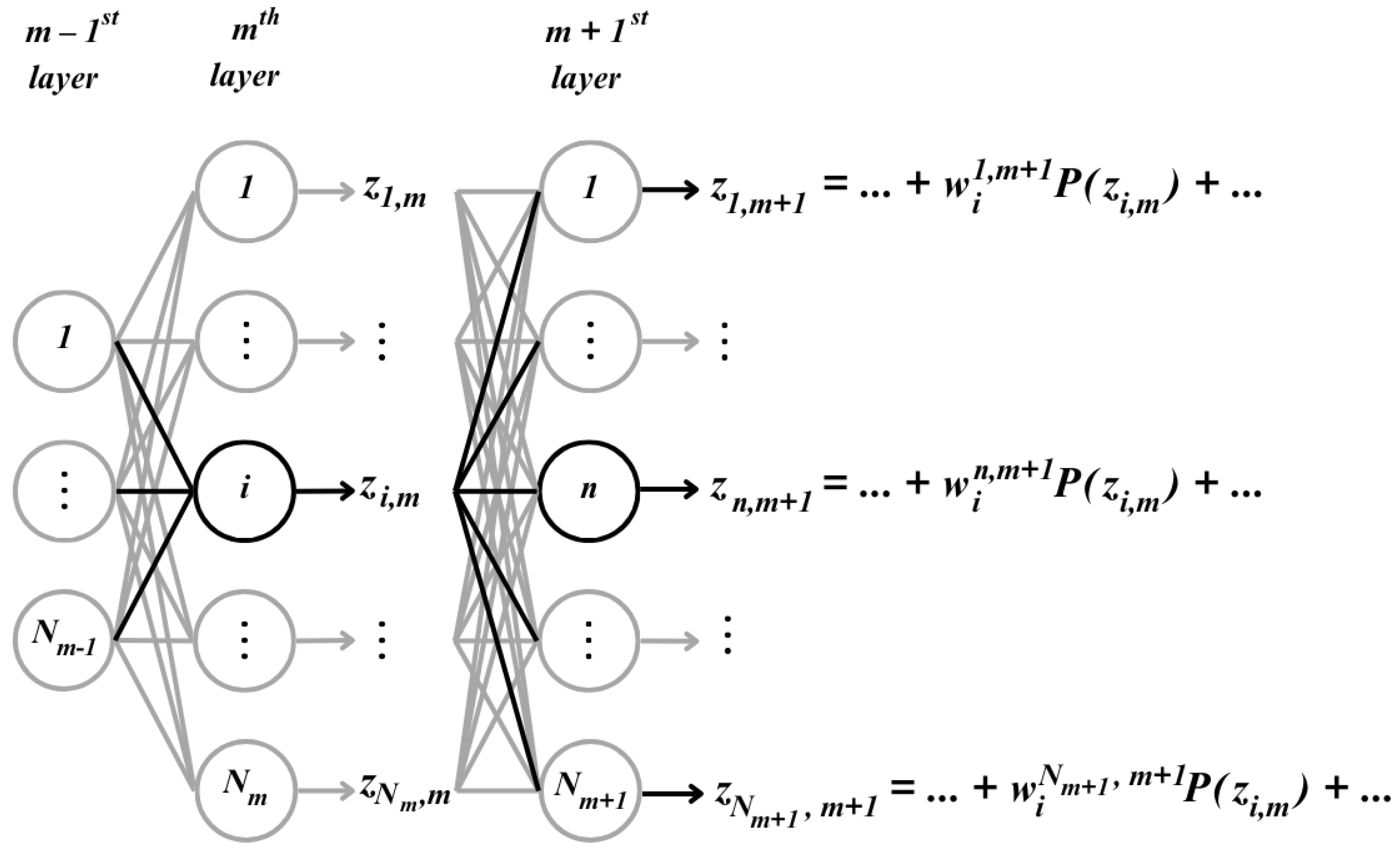
Figure 1. The i t h weights of the m + 1 s t layer neurons are responsible for processing the output of the i t h neuron in the preceding m t h layer.
Algorithms 17 00361 g001
Figure 2. Passing the flattened feature maps to the first fully connected layer (a) is analogous to the same process between the fully connected layers (b).
Algorithms 17 00361 g002
Figure 3. Convolution process of the 4 × 4 image by the 2 × 2 kernel with stride 1. White pixels determine the kernel position, and a yellow pixel is the target pixel. On picture (a), we see a single possible kernel position where the x 11 pixel is involved into a convolution. On picture (b), we can see that pixel x 33 is participating in the convolution four times—every time in a different kernel position.
Algorithms 17 00361 g003
Figure 4. Backward convolution process. The blue square contains the errors of the feature map obtained in the second convolutional layer padded with zeros. The white square is the kernel rotated by 180 ° . The green square represents errors of the feature map in the first convolutional layer.
Algorithms 17 00361 g004
Figure 5. Process of the Fourier coefficients pooling: (a) the Fourier coefficients of the image; (b) Fourier coefficients with circular shift; (c) extraction of the frequencies around DC frequency.
Algorithms 17 00361 g005
Figure 6. CNNMVN accuracy for MNIST dataset with different normalization.
Algorithms 17 00361 g006
Figure 7. CNNMVN accuracy for Fashion MNIST dataset with different normalization.
Algorithms 17 00361 g007
Figure 8. MLMVN as a Frequency domain CNN accuracy for MNIST dataset using 1–5, 1–6, 1–7 frequencies and the original image as input.
Algorithms 17 00361 g008
Figure 9. Accuracy of MLMVN as a frequency-domain CNN for Fashion MNIST dataset using 1–7, 1–8, 1–9 frequencies and the original image as input.
Algorithms 17 00361 g009
Figure 10. Accuracy of MLMVN as a frequency-domain CNN for MNIST with strict batch learning.
Algorithms 17 00361 g010
Figure 11. Accuracy of MLMVN as a frequency-domain CNN for Fashion MNIST with strict batch learning.
Algorithms 17 00361 g011
Figure 12. Comparison of an original image (a) with the frequency-domain downsampled image (d), and results of spatial-domain convolutions performed by CNNMVN (b,c) compared with those of frequency-domain convolutions performed by MLMVN (e,f). Figure description: (a) Original image; (b) After convolution with the 7th kernel; (c) After convolution with the 26th kernel; (d) Original image after frequency-domain downsampling (frequencies 1–5 were used) and inverse Fourier transform; (e) After convolution with the 221st kernel; (f) After convolution with the 366th kernel.
Algorithms 17 00361 g012
Table 1. Classification results for CNNMVN for MNIST dataset.
TopologyPool TypeType of Error
Normalization
Epoch When
Maximum Accuracy Reached
Accuracy
16C5-h128-o10NoneCustom1897.2
16C5-h256-o10NoneCustom1997.18
32C5-h128-o10NoneCustom1997.42
32C5-h256-o10NoneCustom1997.46
32C5-P2-h256-o10Max. poolCustom1096.36
32C5-P2-h256-o10Average poolCustom1994.63
32C5-h256-o10NoneDefault2075.99
Table 2. Classification results for CNNMVN for Fashion MNIST dataset.
TopologyPool TypeType of Error
Normalization
Epoch When
Maximum Accuracy Reached
Accuracy
16C5-h128-o10NoneCustom886.91
16C5-h256-o10NoneCustom1686.99
32C5-h128-o10NoneCustom1387.7
32C5-h256-o10NoneCustom1688.03
32C5-P2-h256-o10Max. poolCustom1386.99
32C5-P2-h256-o10Average poolCustom884.78
32C5-h256-o10NoneDefault2069.2
Table 3. Classification results for MLMVN as a CNN in a frequency domain for MNIST dataset.
TopologyNumber of Frequencies UsedEpoch When Maximum Accuracy ReachedAccuracy
h1024-o10Images transformed by (1)19993.18
h2048-o10Images transformed by (1)19094.13
h1024-o10514597.86
h2048-o10519398.11
h1024-o10618397.91
h2048-o1068598.09
h1024-o10720097.78
h2048-o10715797.86
h1024-h2048-o10513997.18
h2048-h1024-o10513796.85
h2048-h2048-o1054597.3
h2048-h3072-o10518797.58
h1024-h2048-o1064097.08
h2048-h1024-o10612496.9
h2048-h2048-o10611397.41
h2048-h3072-o1069597.44
h1024-h2048-o1072596.68
h2048-h1024-o1073896.66
h2048-h2048-o1076496.71
h2048-h3072-o1076597.15
Table 4. Classification results for MLMVN as a CNN in a frequency domain for Fashion MNIST dataset.
TopologyNumber of Frequencies UsedEpoch When Maximum Accuracy ReachedAccuracy
h2048-o10Images transformed by (1)9187.48
h3072-o10Images transformed by (1)5187.94
h2048-o10717889.81
h3072-o10711890
h2048-o10818089.85
h3072-o10816589.89
h2048-o1094389.99
h3072-o10910990
h2048-h3072-o1072488.87
h3072-h2048-o1072388.63
h2048-h3072-o1088188.51
h3072-h2048-o10814788.19
h2048-h3072-o1093088.5
h3072-h2048-o1096088.18
Table 5. Classification results for MLMVN as a CNN in a frequency domain for MNIST and Fashion MNIST datasets with strict batch learning.
DatasetTopologyNumber of Frequencies Used# of Iteration *
When Maximum
Accuracy Reached
# of
Iterations
Accuracy
MNISTh2048-o1053002323898.2
MNISTh3072-o1052274292897.93
Fashion MNISTh2048-o1074484535189.54
Fashion MNISTh3072-o1073719443589.11
* Epochs are replaced by iterations because each epoch is not determined in this type of learning and can take dozens of iterations.
Disclaimer/Publisher’s Note: The statements, opinions and data contained in all publications are solely those of the individual author(s) and contributor(s) and not of MDPI and/or the editor(s). MDPI and/or the editor(s) disclaim responsibility for any injury to people or property resulting from any ideas, methods, instructions or products referred to in the content.