Abstract
Time series analysis is pivotal for business and financial decision making, especially with the increasing integration of the Internet of Things (IoT). However, leveraging time series data for forecasting requires extensive preprocessing to address challenges such as missing values, heteroscedasticity, seasonality, outliers, and noise. Different approaches are necessary for univariate and multivariate time series, Gaussian and non-Gaussian time series, and stationary versus non-stationary time series. Handling missing data alone is complex, demanding unique solutions for each type. Extracting statistical features, identifying data quality issues, and selecting appropriate cleaning and forecasting techniques require significant effort, time, and expertise. To streamline this process, we propose an automated strategy called Preptimize, which integrates statistical and machine learning techniques and recommends prediction model blueprints, suggesting the most suitable approaches for a given dataset as an initial step towards further analysis. Preptimize reads a sample from a large dataset and recommends the blueprint model based on optimization, making it easy to use even for non-experts. The results of various experiments indicated that Preptimize either outperformed or had comparable performance to benchmark models across multiple sectors, including stock prices, cryptocurrency, and power consumption prediction. This demonstrates the framework’s effectiveness in recommending suitable prediction models for various time series datasets, highlighting its broad applicability across different domains in time series forecasting.
1. Introduction
Time series data, characterized by sequential data points recorded at specific timestamps, present unique challenges in data science, demanding specialized preprocessing techniques to ensure data quality. Time series analysis encompasses data collection, cleaning, preprocessing, and forecasting, tailored to different types of time series, whether numeric or textual, univariate or multivariate, seasonal or nonseasonal. Existing research predominantly focuses on univariate time series, while multivariate time series pose additional complexities such as noise, missing values, outliers, and seasonality. To address these challenges, an automated preprocessing framework integrating various techniques and machine learning algorithms is proposed. Time series analysis, crucial in IoT and financial domains, requires extensive data cleaning and preprocessing due to its distinctive characteristics and challenges. Understanding the properties of the data, such as stationarity and distribution, is essential for selecting appropriate preprocessing techniques. Additionally, deep learning algorithms like GANs and auto-encoders show promising results in preprocessing and forecasting time series data.
The quest for the most accurate forecasting model with minimal error rates in numerical time series analysis requires exhaustive experimentation with various techniques and their combinations. The type of technique applicable to a particular type of data should also be known [1]. However, this process is time-consuming and labor-intensive. Different imputation methods are employed based on the time series properties, such as distribution and seasonality, to handle missing values effectively. With the exponential growth of time series data generated by diverse sources like stock exchanges [2], energy consumption [3], health monitoring systems, and weather recording systems, analysts face increasing workloads. Time series, characterized by sequential data recorded over time intervals, present unique challenges such as handling noise, seasonality, and missing values, which necessitate specialized preprocessing techniques to ensure data quality and improve forecasting accuracy.
Preprocessing, a crucial step in data analysis and machine learning, involves a series of steps to enhance data quality and simplify model training. However, preprocessing is time-intensive, lacks a predefined sequence, and varies across different domains. In the context of time series analysis, preprocessing becomes more complex due to the real-time nature and sequential dependencies of the data. Challenges include handling missing, duplicate, and incorrect data, including outliers. The existing literature predominantly focuses on handling missing data and outlier detection in time series preprocessing.
Outliers, which deviate significantly from the majority of data points, can be univariate or multivariate, with the latter posing greater complexity. Multivariate outlier detection often requires machine learning approaches due to the multidimensional feature space involved. Outlier detection techniques encompass statistical and machine learning methods. Statistical techniques include exponential smoothing, z-score, linear regression models, and interquartile range, while machine learning techniques comprise supervised methods like neural networks and decision trees, and unsupervised methods like cluster analysis. Distance measuring techniques, information theory-based methods, and algorithms like KNN and COF are also utilized.
Handling missing values in time series data involves either removing incomplete records or imputing missing values. Imputation techniques for time series data, including spline interpolation and moving averages, differ from those used in non-time series data due to temporal properties. Traditional methods may not suffice, necessitating advanced techniques like interpolation, auto-encoders, and generative adversarial networks (GANs) for imputation and outlier detection.
Time series data analysis considers properties such as seasonality and trend, categorizing time series into types based on their characteristics. Challenges in time series data extend beyond outliers and missing values to include concept drift, class imbalance, handling trend, and seasonality and data consistency issues.
According to [4], time series analysis is mostly performed using statistical methods; however, machine learning techniques have increasingly gained prominence in time series analysis, promising more accurate results with adequate preprocessing. However, preprocessing remains vital for enhancing data quality and ensuring reliable predictions [5]. Techniques like SCREEN [6] offer constraint-based cleaning methods for time series data, improving accuracy and efficiency in data analysis. Research studies have explored various approaches to enhance preprocessing techniques for time series data. One study [7] utilized meta-learning to select preprocessing alternatives, focusing on transformation effects on algorithm performance across datasets such as Automobile, Credit, Iris, and Vote. While regression trees showed limited effectiveness as a meta-learner, transformations significantly improved outcomes. Another study [8] introduced an iterative minimum repairing and parameter prediction method for anomaly repair, achieving a substantial enhancement in execution speed across datasets including GPS, Intel Lab Data, and China Meteorological data. In a separate investigation [9], Landsat time series imagery combined with trajectory analysis was employed to detect forest instabilities in Myanmar. This study highlighted the correlation between areas of instabilities and harvested trees, indicating potential applications for selective logging. Change detection in time series was comprehensively analyzed [10], covering preprocessing techniques like atmospheric correction and cloud detection, along with popular automated preprocessing algorithms like LEDAPS and Fmask. Augmenting fully convolutional networks with LSTM-RNN was proposed [11] for time series classification, demonstrating improved performance with attention mechanisms. Additionally, studies [12] addressed data profiling issues, proposing visual-based software solutions for data quality checks and outlier detection techniques using methods like the k-sliding window technique and neural networks [13].
A review [14] highlighted the need for further research in time series cleaning tools and systems, emphasizing the importance of preprocessing for maximizing data potential. Potential areas for future work include error data type analysis, multidimensional time series cleaning algorithms, anomaly detection, and specific application data cleaning techniques. Several innovative systems have been proposed to address challenges in cleaning time series data across various domains. Cleanits [15], for instance, focuses on industrial time series data cleaning, utilizing Bollinger bands for anomaly detection and LSTM for repairing errors. While primarily designed for industrial data, there is potential for its application in other domains, requiring flexibility enhancements.
In the energy sector, knowledge extraction systems have been proposed [16] using clustering techniques, with k-Medoids showing promising results on energy time series. Medical science also benefits from time series data analysis, prompting the development of systems like Clairvoyance [17], facilitating rapid prototyping and optimization of clinical decision systems. Hybrid models and systems like AutoMTS have been introduced for cleaning multivariate time series data [18,19], demonstrating their significance in improving data quality through imputation and outlier detection. AutoML and frameworks like DAEMON [20,21] focus on automating machine learning model fitting and outlier detection in time series data, achieving high accuracy and demonstrating potential for online anomaly detection services [22].
Time series data with seasonality pose unique challenges, such as multi-seasonality and heteroscedasticity, which complicate analysis and prediction. Research [23,24] has addressed these challenges by preprocessing data, building models, and adapting them to original measurements, followed by anomaly detection. Further studies aim to enhance local trend prediction and outlier correction in time series analysis. Non-stationarity has been addressed in studies focusing on volatile and non-volatile data cleaning [25]. Techniques like k-nearest neighbors and sliding windows have been explored [26], with sliding windows performing better, particularly for volatile data like stock market time series [27]. Efforts have been made to measure data quality using indices like the Attribute Value Quality Index (AVQI) and Structured Data Value Quality Index (SDVQI), enabling comparison and improvement of data quality measures.
Optimization algorithms like genetic algorithms (GAs) have been employed to automate feature selection in preprocessing, improving regression models’ efficiency [28]. While existing solutions like SCREEN, CLEANITS, DAEMON, and Clairvoyance address specific preprocessing challenges, there is a need for a generic approach spanning multiple domains. Preptimize stands out by offering an integrated solution for preprocessing and model recommendation, making it accessible to non-experts and capable of handling diverse time series challenges. SCREEN and DAEMON focus on anomaly detection and cleaning, while CLEANITS specializes in imputation. Clairvoyance is primarily a forecasting tool utilizing advanced machine learning techniques. Preptimize’s broad applicability and user-friendly approach differentiate it from these specialized tools. Various open-source libraries and proprietary SaaS products automate machine learning pipeline generation and optimization, streamlining the preprocessing process [29,30].
Time series values to be forecasted can be nominal, categorical, textual, and numerical. Numerical forecasting is a regression problem which can be solved using various techniques like moving averages, autoregression, and exponential smoothing, as well as advanced methods like ARIMA, SARIMA, VAR, and LSTM [31]. Hybrid approaches combining statistical and machine learning models are also common [32,33,34]. However, no single technique suits all time series due to their varying properties, making the selection process time-consuming and complex. To streamline the process of analyzing a time series, a standard procedure should be adopted to automate profiling, preprocessing, optimized model forecasting, evaluation, and selection of the best-performing model with minimal error.
The primary contribution of this work is the introduction of Preptimize, an automated strategy for analyzing time series data that integrates statistical and machine learning techniques to recommend optimal models for analysis. By reading a sample from a large dataset, Preptimize suggests blueprint models based on optimization, including the best combination of preprocessing and forecasting techniques, thereby enhancing forecasting accuracy across various types of time series data. Preptimize streamlines the process of analyzing both univariate and multivariate time series with missing values. On basis of the complexity involved in time series analysis, this research highlights the importance of choosing the right forecasting technique and preprocessing strategy based on the type of time series data to expedite the process of analyzing the time series data. Additionally, this work demonstrated the framework’s potential for broad applicability in time series forecasting, supporting its effectiveness in recommending suitable prediction models.
2. Materials and Methods
Based on the discussion in the previous section, it can be determined that a comprehensive framework is essential that can define standard steps during preprocessing and forecasting time series. The subsequent section has a thorough explanation of the proposed framework called Preptimize. The focus of Preptimize is to automate the process of time series analysis by offering the first blueprint model for further analysis. The proposed framework was implemented using the Python programming language.
Preptimize
Preptimize begins by reading time series data and generating a comprehensive profile that includes distribution analysis, seasonality, and trend detection. It then preprocesses the data by addressing data quality issues such as missing values and outliers using various techniques and evaluates the preprocessed data using multiple forecasting models to identify the best-performing model. The steps are also mentioned in Figure 1. Since the framework design is a big task, this paper focuses on numerical data and missing data problems. This work aims to explain most solutions available to handle missing data in time series and gives the best solution possible. The proposed framework is tested on different datasets including cryptocurrency data, stock market data, and an IoT network’s generated data.
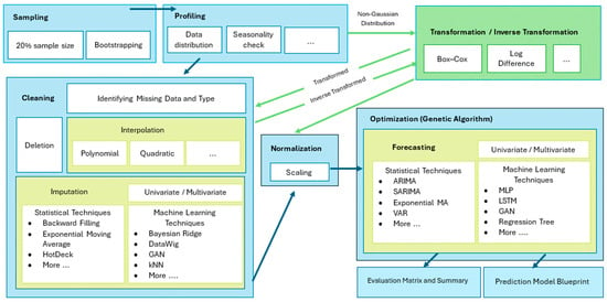
Figure 1.
Preptimize: Visual depiction of the systematic approach integrating preprocessing, model selection, and thorough evaluation stages, enhancing efficiency in time series analysis.
There are numerous techniques and algorithms utilized in the implementation of Preptimize, as outlined in Table 1. The rules that Preptimize follows to recommend potential prediction model blueprints are derived from the existing literature. Therefore, organizing and streamlining these rules and findings is a significant contribution of this work. The basic pseudocode of the proposed framework is given in Figure 2. The following section highlights only the most common techniques employed at various stages of the process.

Table 1.
Details of techniques used in the implementation of Preptimize.
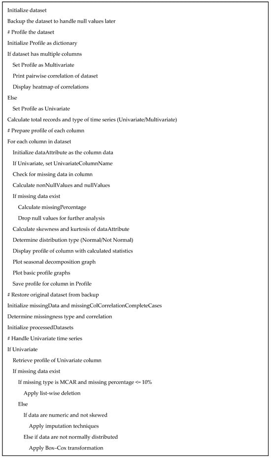
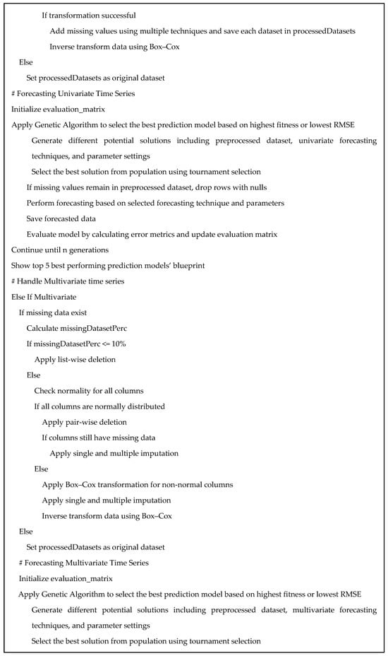
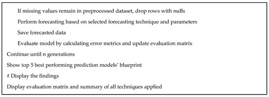
Figure 2.
Preptimize: Sequential workflow for time series data preprocessing and model selection. Here, # represents the comment.
2.1. Data Sampling
In the first stage, Preptimize generates a sample from the data to represent the original behavior while reducing the size to 20%. Bootstrapping was applied, and the index was maintained.
2.2. Data Profiling
In this stage, different properties of data are computed, and a profile is created for the attribute. These properties include mean, median, minimum and maximum value, variance, and standard deviation of the data. Data are further explored by finding the distribution type, skewness, and kurtosis of the data. Stationarity of data is also computed, which includes seasonality and trend. A brief description of these techniques is given below.
2.2.1. Data Distribution
Data distribution specifies all likely values for a variable and also quantifies the relative rate of occurrence indicating how frequently a value is appearing. There are different distributions possible, which can be normal, binomial, Poisson, or Bernoulli distribution. Most of the situations follow the normal distribution, which is expressed as a bell-shaped and symmetrical curve around the line x = μ. It indicates an equal number of values are present on both sides of the center. The Gaussian distribution with a mean of 0 and a standard deviation of 1 is the standard Gaussian distribution.
The two properties linked with distribution are skewness and kurtosis. Skewness is a measure of regularity. The series of data is symmetric if it appears the same on both sides of the midpoint. Kurtosis measures the rate of occurrence of outliers at the tail. Data with heavy tails indicate more outliers, and the value of kurtosis is high. The kurtosis of a normal distribution is 3. If less than 3, there are few outliers, and if greater than 3, there are more outliers. Skewness can be negative, which specifies that the tail is on the left side; otherwise, the tail is on the right. If skewness is zero, then the distribution is perfectly symmetrical. The distribution can be considered normal if the values of skewness fall between −3 and +3, and kurtosis is in a range of −10 to +10 when utilizing the standard error of measurement [35].
2.2.2. Stationarity
A time series whose traits are not subject to time is stationary. Thus, the presence of a trend or seasonality indicates the series is not stationary. The observed property at different times gets affected by trend and seasonality. A time series has three components, which are season, trend, and noise. The season can be defined as the reiterating short-term cycle in the series. The trend is the slope in the data, which can rise or decline with time, whereas the noise is the random change in the series. It is often considered challenging to deal with time series data that contain seasons or trends. Plotting the time series gives instant information about the presence of a season and a trend.
There are two common approaches to deal with seasonal time series. One method is to split the series by removing the seasonal and trend component and then use the series for analysis or use any other transformation technique to obtain the nonseasonal representation of the series. The other way is to use specially designed forecasting techniques for seasonal series like SARIMA.
2.2.3. Identifying the Type of Missing Data
In handling missing data, three categories are identified: missing completely at random (MCAR), missing at random (MAR), and missing not at random (MNAR). In univariate analysis, treating time as a variable adds complexity, requiring consideration of time series traits and covariance for imputation. For MCAR data, univariate imputation is relatively straightforward. However, in multivariate analysis, the association between columns is taken into account. MCAR data are randomly missing and can often be replaced with mean or median values, as the missing data are considered recoverable. MCAR is given by (1), where R is missing data and Y is the complete data.
MCAR data lack significant association according to measures like Chi-Square, Cramer’s rule, or the correlation coefficient, and typically contain fewer null values. For large datasets, instances with missing data may be omitted or imputed. Deletion methods for MCAR include list-wise deletion, removing records with any null value, suitable when missing data are minimal, and pairwise deletion, retaining data for pairs of quantities with available data points, preserving more data. Imputation becomes necessary when deletion methods are unsuitable. Imputation involves substituting missing data with expected values, with various techniques applied depending on the nature of the data. In the case of MAR, missing data may follow a pattern or sequence, occasionally appearing outside the sequence. When a relationship between missing and existing data is identified, it is considered MAR. Imputation techniques such as mean, median, mode, or interpolation can be employed to handle MAR, with multiple imputation techniques available for non-time series data and interpolation for time series data. MAR is given by (2)
P(Ri|Yi) =P(Ri|Yi,o)
In MNAR, specific instances share missing data, making prediction challenging as it relies on unobserved information. If missingness in one column shows little or no correlation with other columns and no strong associations are found upon investigation, and the frequency of missing values is high, this is considered MNAR. MNAR is non-ignorable, with no straightforward method for handling it other than obtaining the missing data. MNAR typically has more null values compared to MCAR and can only be identified through domain knowledge. MNAR is given by (3):
P(Ri|Yi) ≠ P(Ri|Yi,o)
2.3. Data Visualization
Utilizing various graphs and plots is a valuable approach in time series analysis for understanding data behavior and properties. Preptimize generates a range of visualizations, such as scatter plots, line plots, and decomposition graphs, to provide a comprehensive overview of the time series data. These visual tools help in understanding data behavior, identifying trends and seasonality, and selecting appropriate preprocessing techniques.
The first set of plots offers an overarching perspective of the data, including scatter plots, line plots, box plots, and histograms. Each attribute in a multivariate time series is plotted individually to capture the data’s essence.
Another crucial plot displays the data distribution, facilitating the assessment of normality. This evaluation is essential for determining suitable statistical techniques.
A graph illustrating season and trend decomposition is particularly helpful in identifying seasonal patterns within the time series. This insight guides the application of appropriate techniques tailored to seasonal data, potentially necessitating transformations for improved analysis.
To assess data stationarity, Preptimize generates a graph plotting rolling mean and rolling standard deviation against the original data. Stationarity is indicated if these values remain constant over time [36].
The heatmap visualization depicts correlations between multiple variables, with higher correlation levels represented by distinct colors. This aids in understanding the strength of relationships between variables.
Additional graphs focus on missing data, including a matrix and bar plot, which provide insights into the nature of missing data and their potential relationships with other attributes.
2.4. Data Cleaning
The preprocessing phase in time series analysis involves data cleaning addressing various data quality issues such as missing values, outliers, and noise. Unlike other forms of data analysis, time series preprocessing requires specific techniques tailored to their unique characteristics. Preptimize employs a range of imputation techniques to handle missing data, including and not limited to linear interpolation, spline interpolation, and machine learning methods such as GANs. The choice of imputation method is based on the specific characteristics of the dataset, ensuring the best possible data quality for forecasting. With nearly 25 different interpolation techniques available, the framework aims to explore the most suitable approach for each dataset. Transformation techniques are applied when data deviate from normality or exhibit non-stationarity. The Box–Cox transformation is utilized to address non-normality, while methods such as seasonal decomposition are employed to remove trends and seasonality from non-stationary data.
Machine learning approaches, including generative adversarial networks (GANs), are integrated into the framework to enhance missing data prediction. For multivariate time series, iterative imputation models and DataWig are utilized to address missing data challenges.
To determine the optimal imputation technique, a comprehensive evaluation is conducted, considering forecasting performance and evaluation metrics. Alternatively, a brute force approach can be employed to test all possible imputation techniques.
Overall, the preprocessing phase plays a crucial role in preparing time series data for analysis and forecasting, necessitating specialized techniques tailored to their unique characteristics and challenges.
2.4.1. Forward and Backward Filling
Last observation carried forward (LOCF) is a widely used single imputation technique that imputes the last measured value by forward filling. There must be at least one post-baseline measure in LOCF. Next observation carried backward (NOCB) is an analogous method to LOCF but works in the reverse direction by backward filling; that is, it uses the first recorded value after the unavailable value and carries it backward.
2.4.2. Interpolation
Interpolation techniques offer a means to predict missing data points by estimating values between known data points. Linear interpolation, the simplest method, connects adjacent points with straight lines, assuming that the points on the line represent the missing values. Polynomial interpolation, which is more versatile, uses polynomial functions of varying orders to represent relationships between attributes. Lagrange polynomial interpolation and Newton polynomial interpolation are examples of polynomial interpolation methods. Lagrange interpolation, while versatile, may struggle with larger datasets.
Newton polynomial interpolation utilizes a recursive division process to construct complex polynomials, which can be effective for prediction but may lead to numerical complexities and sensitivity to outliers. Spline interpolation, on the other hand, utilizes piecewise polynomials to fit smoother curves to smaller groups of data points, with cubic spline interpolation often preferred for its smoothness and stability.
Other interpolation methods employed in the framework include piecewise polynomial, Akima, Barycentric, Krogh, and Pchip, each offering different approaches to estimating missing values in time series data.
2.4.3. Moving Average
Moving averages, such as simple moving averages (SMAs), cumulative moving averages (CMAs), and exponential moving averages (EMAs), are commonly used for imputation in time series analysis. SMA calculates the average of a specified number of data points, using a simple summation formula. CMA computes the average for all entries up to the current time, with each value equally weighted. EMA employs exponentially decreasing weighting factors to compute the average, with the value at any time determined by a coefficient and the previous EMA value. These moving averages can aid in data imputation, provided the time series is stationary. Stationarity, indicating consistent behavior over time, can be assessed using statistical tests like the Augmented Dickey–Fuller (ADF) test [37] or by observing rolling statistics, such as rolling mean and standard deviation plots.
2.4.4. Deep Learning Algorithms
Data imputation using deep learning techniques, particularly recurrent neural networks (RNNs) and generative adversarial networks (GANs), has emerged as a promising approach in recent literature for time series analysis. RNNs and their variations excel in modeling sequence data, while GANs are adept at generating and imputing missing values. Preptimize leverages a GAN for both single and multiple imputations. The GAN operates through two models, the generator (G) and discriminator (D), which work adversarially to generate realistic data samples and distinguish between real and fake samples, respectively. Training continues until the discriminator is unable to differentiate between real and generated samples, indicating the generator’s ability to produce credible examples.
In GANs, D tries to assign the correct label to the samples with maximum probability, whereas G tries to minimize log (1 − D(G(z))). According to [38], D and G play the two-player minimax game with value function V (G, D), as shown by (4).
In Preptimize, a model presented in [39] is used for imputing missing data using a GAN. The method is called Generative Adversarial Imputation Nets (GAIN). In the method, G observes real data, imputes the missing element, and outputs finalized data. D then takes a finalized datum and tries to discover which elements are observed and which are imputed.
2.4.5. Multiple Imputation
Multiple imputations (MIs) offer a comprehensive approach to handling missing values by utilizing the complete set of features to approximate the missing values. MI generates multiple datasets by imputing missing values, allowing for the replacement of missing values with multiple possible values. These imputed values are estimated from each dataset and then aggregated into a final dataset. MI is applicable in cases where the data are missing completely at random (MCAR), when they are missing at random (MAR), and even when the data are missing not at random (MNAR).
Iterative imputation, on the other hand, involves modeling each feature as a function of the other features in a sequential process. Past imputed values are used to predict succeeding features until all missing values are filled. Preptimize utilizes the IterativeImputer library in Python, which offers various estimators such as the Bayesian Ridge regressor, random forest regressor, K-neighbors regressor, decision tree regressor, and Extra Trees regressor.
Additionally, the KNNImputer technique, provided by the same Python library, employs the k-nearest neighbors approach to impute missing values by considering values of observations for neighboring data points.
DataWig, another method used for imputation, has shown effectiveness in the literature for imputing missing values. DataWig [40] is a deep learning library that leverages MXNet as a backend to generate predictions for missing data.
Furthermore, the hot deck [41] method, known for its computational efficiency, is utilized for imputation. This method imputes missing values by selecting a randomly similar record within a data matrix and using existing values from the donor object. The hot deck operates on one attribute at a time and serves as a single imputation technique.
2.5. Forecasting
There are various prediction approaches that exist in the literature for time series. Examples encompass exponential smoothing, the autoregressive integrated moving average (ARIMA) with seasonal and nonseasonal variants, multiple deep learning techniques, and many others. There are separate techniques for forecasting a univariate and multivariate time series. Preptimize uses a genetic algorithm [42] to explore the vast space of possible models and configurations to find the most suitable one for a given dataset. Each individual in the population represents a potential solution comprising a preprocessing strategy, a forecasting model, and parameter settings. Each individual is evaluated based on a fitness function, which in this case is the RMSE. The lower the RMSE, the better the model. Individuals are selected based on their fitness scores to be parents for the next generation. Mutation is performed based on the bit-flip scheme; 3 individuals are selected from the population at random using tournament selection. This approach helps in automating the model selection process, potentially saving significant time and effort while achieving optimal or near-optimal forecasting accuracy.
2.5.1. Univariate Forecasting
Univariate forecasting involves predicting future values of a single variable based on historical data from consecutive time intervals. The choice of forecasting technique depends on whether the time series exhibits seasonality and trend components.
Two main types of univariate forecasting methods exist: statistical methods and advanced machine learning-based methods. Statistical methods include autoregression (AR), moving average (MA), autoregressive moving average (ARMA), autoregressive integrated moving average (ARIMA), and simple exponential smoothing. Moving average techniques such as simple moving average, exponential moving average, and cumulative moving average are common.
For time series with seasonality and trend, options include seasonal autoregressive integrated moving average (SARIMA), seasonal autoregressive integrated moving average with exogenous regressors, and Holt–Winters exponential smoothing (HWES), with ARIMA and SARIMA being the most successful.
ARIMA combines autoregression, moving average, and differencing to achieve stationarity. Proper identification of ARIMA parameters (p, d, q) is crucial, typically performed by fitting models with different orders using criteria like the Akaike information criterion (AIC) to select the best order. The AIC measures model performance relative to the number of parameters. The autocorrelation function (ACF), and partial autocorrelation function (PACF) cannot be used to identify reliable values for p and q [43]. Residual analysis is essential in ARIMA modeling to ensure residuals resemble white noise, indicating no autocorrelation. The Ljung–Box test is commonly used to assess residual autocorrelation, where p-values above a threshold suggest no significant autocorrelation.
Time series forecasting has garnered significant attention in machine learning and deep learning. Preptimize also considers these ML-based methods of forecasting. The literature presents various techniques for this purpose, including Long Short-Term Memory (LSTM), support vector regression (SVR), the multi-layer perceptron (MLP), decision trees, random forest, the recurrent neural network (RNN), and its variant the Gated Recurrent Unit (GRU).
Among these techniques, LSTM stands out, known for its effectiveness in handling sequential data. However, traditional RNNs face challenges like vanishing and exploding gradients, leading to longer training times and lower precision. These issues are addressed by LSTM and GRU, which are more efficient in managing gradient problems.
GRU differs from RNNs in its use of update and reset gates to control information flow and address gradient issues. These gates determine how much preceding information is retained or discarded, enhancing the model’s efficiency. Variants of GRU, including bidirectional versions, are utilized in the proposed framework.
LSTM, another variant of RNN, comprises multiple LSTM units, each equipped with cell, input, output, and forget gates. These gates play a crucial role in the LSTM model, facilitating the sequential processing of data and prediction generation.
This framework employs various configurations of neural networks for forecasting, including Vanilla LSTM, Stacked LSTM, Bidirectional LSTM, and CNN-LSTM. Vanilla LSTM consists of one hidden layer and one output layer, while Stacked LSTM involves multiple hidden layers. Bidirectional LSTM processes data in both forward and backward directions and then combines the interpretations. CNN-LSTM integrates a CNN to understand sequence parts and then passes them to LSTM for interpretation, forming a hybrid model.
Comparing GRU and LSTM, no clear winner emerges across all performance parameters. GRU executes faster with fewer parameters and less memory usage, while LSTM demonstrates greater precision, especially on larger datasets.
MLP serves as a foundational artificial neural network, featuring fully connected feedforward layers suitable for classification and regression tasks. It comprises at least an input layer, a hidden layer, and an output layer, utilizing nonlinear activation functions to handle linearly non-separable data.
For regression tasks, support vector regression (SVR) offers flexibility in defining error tolerance, seeking to minimize the L2-norm of the coefficient vector while allowing for deviations with slack variables. Decision trees, including regression trees, are employed for forecasting time series, while random forest combines multiple regression trees to enhance prediction accuracy through bagging and feature randomness.
2.5.2. Multivariate Forecasting
In the proposed framework, multivariate time series forecasting utilizes a range of statistical and machine learning methods. While statistical approaches for multivariate time series are limited, the framework incorporates key techniques like vector autoregression (VAR), vector moving average (VMA), and vector autoregression moving average (VARMA).
Unlike univariate techniques such as AR and ARIMA, vector-based methods like VAR, VMA, and VARMA are bidirectional, allowing variables to influence each other. However, these techniques require stationarity, often confirmed using the ADF test. VAR establishes relationships between variables through a system of equations, with lag selection guided by criteria like Akaike information criterion (AIC). VMA operates with a moving average matrix and a k-dimensional vector, while VARMA integrates both autoregressive and moving average orders. For machine learning-based forecasting, the framework employs techniques like MLP, regression tree, random forest, RNN, GRU, and LSTM, each detailed in the preceding section.
3. Experimental Results and Discussion
This study evaluates Preptimize, a framework designed for time series data analysis, across various domains and scenarios including stock market data, cryptocurrency data, and IoT-generated power consumption data. Each experiment involves preprocessing the data, applying various forecasting techniques, and assessing the performance using metrics such as MAE, MSE, RMSE, and MAPE. The details of datasets used are mentioned in Table 2. The framework employs preprocessing and forecasting techniques tailored to each dataset type, with the selection optimized through a genetic algorithm (GA). Preptimize is designed to leverage the GA for optimizing model selection. To ensure a comprehensive understanding of the framework’s functionality, all possible models were evaluated. The GA was adapted to include all potential models, identifying both the best and worst performers. This was achieved by assigning the highest value to the top-performing models. In practical applications, however, the GA typically recommends the five best-performing models based on the lowest RMSE, balancing efficiency and effectiveness. Evaluation metrics include MAE, MSE, RMSE, and MAPE, with detailed analysis provided in a comprehensive report generated by Preptimize. Experiments are conducted separately for univariate and multivariate datasets, covering the stock market, cryptocurrency, and home-based power consumption data. Each experiment is meticulously described, including dataset details, training/testing procedures, and evaluation outcomes. The details and findings of these experiments are given below.

Table 2.
Details of datasets used in experiments.
3.1. Experiment 1: Univariate Series
Preptimize underwent initial testing on market data including stock and cryptocurrency, a common type of time series data characterized by the fluctuating prices of listings over time. Experiment 1 is divided into three parts. Part 1 utilized complete stock data to assess Preptimize’s performance on high-quality data. Part 2 introduced intentionally missing data to evaluate the framework’s handling of incomplete datasets. Part 3 employed cryptocurrency data with missing values to further test Preptimize’s capabilities. These experiments aimed to gauge the framework’s effectiveness across various scenarios and data qualities in the domain of financial prediction.
In the first part of the experiment, this study explores stock market data from Yahoo Finance, focusing on the Microsoft Corporation (MSFT), listed on the NASDAQ exchange. Using the yfinance Python library, market data from August 2020 to August 2022 were collected, specifically examining the closing prices on each trading day, excluding weekends. This constitutes a univariate time series dataset, comprising around 500 records, which were divided into training and test sets. Notably, the dataset was complete and devoid of quality issues, obviating the need for preprocessing in the initial phase of the experiment.
A total of 139 models were employed to forecast the time series, with the generated report providing an extensive overview of the data analysis process. Despite space limitations, the report includes essential features such as basic profile characteristics, rolling mean and standard deviation graphs, scatter plots, box plots, distribution graphs, and trend decomposition graphs. Moreover, the report encompasses training logs, error calculations, and performance evaluations for all models. Figure 3a,b illustrate the distribution of the data, indicating normalcy, and depict the decomposition of trend and seasonality within the time series. Comprehensive analyses, including p-values and Augmented Dickey–Fuller (ADF) statistics, suggest the stationarity of the time series with no discernible seasonality. The model performance summary file had results of about 139 models, out of which a few are mentioned in Table 3, showing only the best 5 and worst 5 performers.
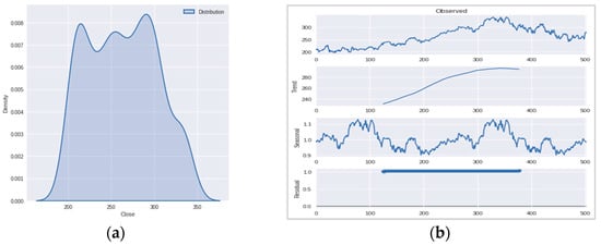
Figure 3.
(a) The graph shows normal data distribution of MSFT closing prices for 2 years. (b) Decomposition graph of closing prices to split the trend and seasonality component. The graph represents a clear upward trend and no seasonality.

Table 3.
Model performance summary of experiment based on univariate time series.
Various forecasting techniques were applied to a univariate stock market dataset, encompassing both machine learning and statistical methods. Machine learning techniques such as LSTM, GRU, and MLP, along with statistical methods like simple moving average, exponential moving average, and ARIMA, were tested with different hyperparameters including hidden layers, neurons, and epochs. Similarly, various variants of statistical techniques were evaluated, such as different orders for ARIMA. These models underwent evaluation on the test dataset using diverse metrics.
The results indicated that the Vanilla LSTM deep learning model performed best on the dataset, achieving an RMSE of 0.0294 with 50 epochs and 40 units. The predicted values generated by this model were compared with the expected values on the test set, as shown in Figure 4a. Among the statistical techniques, exponential moving average (EMA) performed the best, with an MAE of 2.0925 and an RMSE of 2.5814. EMA was ranked 127th out of 139 models. Conversely, the cumulative moving average (CMA)-based model exhibited the worst performance, with an MAE of 27.2085 and an RMSE of 35.1176. Figure 4b depicts a comparison between the actual values and the forecasted values produced by the CMA model.
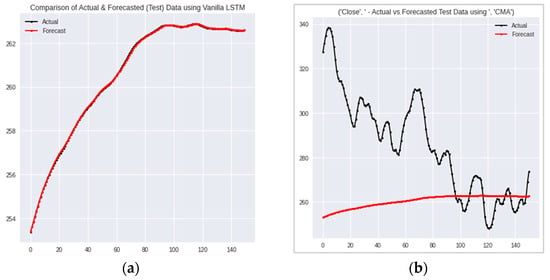
Figure 4.
(a) Comparison of actual and forecasted data generated by Vanilla LSTM using 50 epochs and 40 units. (b) Comparison of actual and forecasted data generated by cumulative moving average (CMA).
ARIMA stands out as one of the most effective and efficient techniques for time series forecasting. In Preptimize, ARIMA was implemented with an optimized order of (2, 1, 2), validated through the Ljung–Box test. However, despite these optimizations, the resulting RMSE of 3.6001 was not particularly impressive.
The stock market dataset was used in the second part of the experiment with missing data problems. As mentioned previously, the data were intentionally removed to test the framework performance by comparing them with the original data.
Preptimize was applied to this dataset containing the missing tuples; the framework generated a report of more than 3500 pages with a detailed description of the steps that were applied to the given dataset, including preprocessing and final analysis. Along with other particulars, the report included details of the missingness type of the data. The framework summarized the data as missing completely at random (MCAR), normally distributed, and stationary, having no season and trend. Figure 5a,b show the trend and season split of the time series and the distribution of the data, respectively.
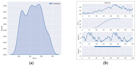
Figure 5.
(a) Decomposition graph of closing price to split the trend and seasonality component. The graph shows a slight upward trend and no seasonality. (b) The graph shows normal data distribution of closing price data.
The summary of the performance of all models applied to the data was computed and stored on a sheet. The summary sheet showed there were about 1270 models applied. These 1270 models were generated as a result of different combinations formed by preprocessing and forecasting techniques. For instance, first, a preprocessing strategy like forward fill was applied to impute the missing data, then all other forecasting techniques were applied for univariate forecasting, including statistical and machine learning techniques, and then each model was evaluated using four different metrics of performance evaluation.
The experiment involved trying multiple preprocessing techniques and models, including interpolation, forward and backward filling, moving averages, and deep learning techniques like GAN for imputation. Each model underwent evaluation on the test dataset using various metrics. The results indicated that ARIMA (p, d, q) with order (7, 1, 2) performed best when missing data were imputed using CMA. The Ljung–Box test confirmed the absence of autocorrelation in the white noise and model. This ARIMA model yielded an MAE of 0.56997 and RMSE of 0.6099. The top five models predominantly belonged to ARIMA, utilizing different imputation techniques such as spline order 3, polynomial order 5, backward filling, and padding. After ARIMA, the exponential moving average performed well with multiple imputation techniques including linear, slinear, piecewise polynomial, and derivative techniques. The first 85 models, which performed well, were all statistical models. Conversely, the CMA-based model processed by a polynomial with degree 9 performed the worst, with an MAE of 28.4643 and RMSE of 36.5159. Figure 6 illustrates the performance of the best and worst models in the experiment, with Figure 6a displaying the values predicted by the ARIMA (7,1,2) model on the dataset imputed by CMA compared with the original values of the test set, while Figure 6b showcases the performance of the CMA model. Support vector regression with a polynomial kernel model imputed using time interpolation emerged as the best in the machine learning category, yielding an MAE of 3.6430 and RMSE of 4.7306. The errors computed for the mentioned models are tabulated in Table 2.
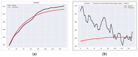
Figure 6.
(a) Comparison of actual and forecasted data generated by ARIMA (7,1,2) imputed by CMA. (b) Comparison of actual and forecasted data generated by CMA imputed by polynomial interpolation of degree 9.
The third part of the experiment focused on analyzing cryptocurrency data, particularly Bitcoin (BTC-USD) from the Coinbase exchange. Cryptocurrency operates independently of traditional banking systems, utilizing blockchain technology for transaction authentication and record keeping. The dataset, spanning approximately two years from Aug 2020 to Aug 2022, consisted of 747 records of Bitcoin prices in USD. To evaluate the framework’s performance in handling missing data, 30% of the dataset was randomly removed. Preptimize processed the data, identifying them as stationary with no discernible seasonality or trend. Despite the dataset’s numeric nature and absence of skewness, it exhibited considerable variance, indicating significant price volatility over the period. Figure 7a,b show the trend and season split of the time series and distribution of the data, respectively. Various imputation techniques, including deep learning methods, interpolation, and moving averages, were employed to address the missing values, with the dataset subsequently split into training and testing sets for forecasting. A total of 892 models were trained and evaluated, with Bidirectional LSTM combined with GAIN imputation emerging as the top performer, achieving an RMSE of 10.028 and MAE of 9.0879. Among statistical techniques, autoregression (AR) showed promise when paired with cubic interpolation, ranking at 693. Conversely, the CMA-based model with spline interpolation and a fifth-degree polynomial exhibited the poorest performance, with an RMSE of 9344.1381 and MAE of 7431.54. Notably, tree-based machine learning algorithms performed suboptimally, with the decision tree regressor and random forest models ranking at 703 and 729, respectively, as shown in Table 2. Performance graphs of the best and worst models are provided in Figure 8.
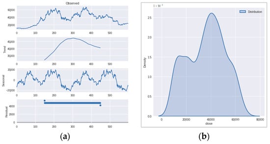
Figure 7.
(a) Decomposition graph of closing prices of Bitcoin (b) Data distribution: the graph shows normal data distribution of Bitcoin’s closing price in USD.
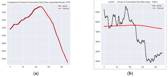
Figure 8.
(a) Comparison of actual and forecasted data generated by Bidirectional LSTM imputed by GAIN. (b) Comparison of actual and forecasted series generated by CMA imputed by spline of 5th-degree polynomial.
The results indicate that Preptimize performs well across different types of time series data. For instance, the Vanilla LSTM model showed the best performance on stock market data, with an RMSE of 0.0294, while ARIMA models with various imputation techniques performed best on datasets with missing values, highlighting the framework’s versatility and effectiveness.
3.2. Experiment 2: Multivariate Series
The second experiment focused on evaluating Preptimize’s performance on multivariate time series data, with and without missing values. The complete data from the stock market were used in the first part, while the second part introduced missing instances using a dataset on individual household electric power consumption.
In the first part, the stock market dataset captured Microsoft’s (MSFT) performance based on open, high, low, and close values from August 3, 2020, to August 1, 2022, totaling 503 records. Preptimize began with data profiling, revealing high pairwise correlation among the columns, indicating dependence. However, ‘open’ and ‘high’ columns were found to be non-stationary, potentially containing trend and seasonality components, as depicted in Figure 9; the heatmap illustrates the pairwise correlation.
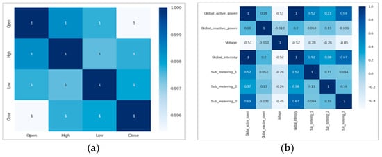
Figure 9.
(a) Correlation heatmap showing correlation between pairs in stock market multivariate dataset. (b) Correlation heatmap showing correlation between pairs in power consumption multivariate dataset.
Moving to forecasting, as no preprocessing was needed, Preptimize applied various techniques including VAR, VMA, VARMA, MLP, decision tree regressor, random forest, RNN, GRU, GRU-bidirectional, and Stacked LSTM. Transformation was applied to ‘open’ and ‘high’ columns to make them stationary before forecasting. Among the models mentioned in Table 4, GRU with 50 units and 100 epochs emerged as the best performer, with 3.9242 MAE and 5.1312 RMSE. Figure 10a showcases the performance of the GRU model on the multivariate test set. However, statistical models like VAR, VMA, and VARMA showed poor performance, failing to understand the basic pattern in the multivariate series. Figure 10b showcases the performance of the VAR model on the multivariate data. Furthermore, the individual columns’ performance analysis indicated that the ‘open’ and ‘high’ columns, initially deemed non-stationary, posed challenges for prediction. Despite applying difference transformation, these columns exhibited predicted values diverging significantly from the original data, leading to high RMSE values.

Table 4.
Model performance summary of experiment based on multivariate series.
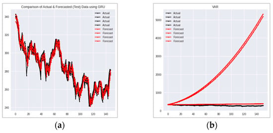
Figure 10.
(a) GRU performance comparison for multivariate time series data during testing. (b) VAR model performance comparison for multivariate time series data during testing.
The second part of the multivariate series experiment tested Preptimize using the individual household electric power consumption dataset, aiming to understand its behavior with incomplete multivariate time series data [44]. This dataset comprises seven columns, excluding date and time, recording power consumption over four years with a one-minute sampling rate. With around 2,075,259 instances, the dataset exhibited missing values primarily in April 2007. Details are given in Table 5.

Table 5.
Individual household electric power consumption dataset used in Experiment 2.
Due to the dataset’s size, only one week of data containing missing instances was processed. With 40 preprocessing strategies and 25 forecasting models, a total of 1000 models were evaluated. However, due to computational limitations, the experiment was split into parts, taking several days to generate results. After conducting previous experiments, 18 successful preprocessing techniques were combined with 25 forecasting models for evaluation.
The comprehensive report generated by Preptimize began by profiling the data, analyzing each attribute individually. A correlation heatmap, depicted previously in Figure 8b, illustrates the pairwise relationships between columns. Notably, global intensity and global active power exhibited a strong positive correlation, while sub-metering 3, associated with climate control systems, correlated strongly with global active power and global intensity. In contrast, global reactive power showed no correlation with other attributes, particularly voltage and sub-metering 3.
Furthermore, the report assessed the missing data percentage, approximately 37%, identifying columns such as sub-metering 1 and sub-metering 2 as non-normally distributed with high kurtosis values. Preptimize classified all four columns with missing data as MNAR type. Attempts to normalize sub-metering 1 and sub-metering 2 distributions were hindered by the possibility of zero or negative values, precluding Box–Cox transformation.
After trend and season decomposition, various imputation techniques, including iterative methods, were applied. Each imputed dataset underwent evaluation using 18 different forecasting models, resulting in a comprehensive performance assessment.
Preptimize generated an evaluation sheet encompassing 450 models, detailing the preprocessing techniques employed during imputation. As shown previously, Table 3 presents the performance metrics of select models, highlighting the best-performing model as GRU imputed with an exponential moving average, yielding an RMSE of 0.6393 and MAE of 0.1225. Conversely, the decision tree regressor, imputed with polynomial interpolation of degree 3, exhibited the poorest performance, with an RMSE of 14.5308 and MAE of 58.7152.
Remarkably, statistical models demonstrated consistent performance when data were imputed using KNNImputer with two neighbors, with VMA, VARMA, and VAR ranking closely. However, some machine learning models fared worse. Performance graphs for GRU and decision tree regressor models are provided in Figure 11a,b, respectively.
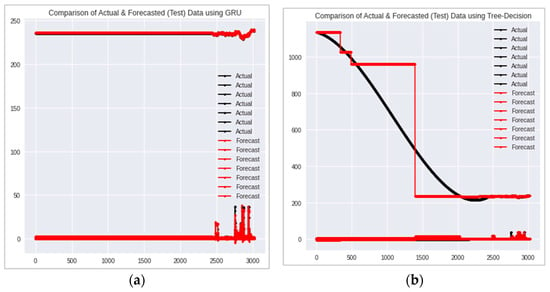
Figure 11.
(a) GRU imputed with exponential moving average: performance comparison for power consumption series data during testing. (b) Decision tree imputed with polynomial interpolation of degree 3: performance comparison for power consumption series during testing.
In summary, the experiment revealed exponential moving average, Bayesian Ridge, KNN-based techniques, and DataWig as effective imputation methods, while polynomial interpolation of degree 3, spline interpolation with degree 3, and HotDeck yielded suboptimal results.
4. Conclusions and Discussion
Time series analysis has grown increasingly intricate due to the multitude of techniques available. Choosing the appropriate forecasting method and preprocessing strategy based on the characteristics of the time series is crucial for obtaining reliable results. Proper steps must be followed in time series analysis to identify the best models applicable in practical settings. Statistical and machine learning models, along with various imputation techniques for handling missing data, offer diverse options for analysis. With abundant research detailing each technique’s performance on specific datasets, there is a need for a system capable of efficiently applying these techniques to identify the best model through optimization.
Through experiments on various time series datasets, the efficacy of the proposed framework, Preptimize, is evident. Preptimize recommends multiple blueprints for prediction models, serving as a preliminary step towards analyzing the given time series and saving significant time and effort. Researchers can further enhance these models by creating hybrid combinations, tuning parameters, and adding more features to improve forecasting accuracy. Preptimize generates detailed reports covering all data processing steps, along with charts, graphs, statistics, and a comprehensive evaluation sheet showcasing the performance of all models tested on the dataset using different error metrics.
Different experiments were conducted on various datasets to evaluate the performance of this framework. The effectiveness of the framework can be judged by how closely the blueprint model matches those used in the literature and by comparing the accuracy based on RMSE. Benchmark performances for stock market prediction models are based on LSTM, SVR, and hybrid models combining statistical methods with machine learning techniques, often reporting RMSE values as low as 0.02 for stock prices. Preptimize also suggested LSTM and ARIMA for stock price forecasting. Benchmark performances for Microsoft (MSFT) stock prediction reported an RMSE of 0.05 with a hybrid model combining LSTM and RNN [45]. The blueprint model proposed with Preptimize achieved an RMSE of 0.029 using Vanilla LSTM. Bitcoin’s high volatility, with significant price fluctuations over short periods, makes it challenging for traditional forecasting models. Bitcoin price prediction reported RMSE values ranging from 4 to 7 for LSTM and random forest models. Preptimize suggested LSTM (RMSE 10.02) for Bitcoin prediction, aligning with findings in the literature. A study [46] reviewed various forecasting models, including feedforward neural networks, LSTM, GRU, ARIMA, and AI techniques, on an individual household electric power consumption dataset to compare their performance. The average RMSE across 12 different models was 0.83, with the lowest RMSE of 0.75 achieved by both LSTM and GRU. In contrast, Preptimize recommended using GRU preprocessed by exponential smoothing, which resulted in an RMSE of 0.639. Based on the discussion, we can conclude that Preptimize effectively recommends suitable prediction models for a given dataset, facilitating rapid decision making with minimal effort.
Preptimize has certain limitations that should be acknowledged. Firstly, it is resource-intensive, requiring significant computational power and time due to its comprehensive approach of applying numerous techniques on a data sample to identify the optimal preprocessing and forecasting methods. Secondly, Preptimize primarily supports datasets with a normal distribution. When dealing with non-normal distributions, it transforms the series to approximate normality, which can add complexity and potential inaccuracies, especially if the transformation does not fully achieve a normal distribution. We aim to address these in future work.
While the proposed framework focuses on addressing the missing data problem in time series analysis, numerous other challenges such as outlier detection, concept drift, and heteroscedasticity persist. Addressing these challenges requires further automation of time series analysis, a task that will be pursued in future phases of research. Future work could explore extending Preptimize to handle more complex types of time series data, such as those with multiple seasons or irregular intervals. Additionally, integrating more hybrid models based on machine learning techniques and expanding the framework’s applicability to other domains like healthcare and environmental monitoring could further enhance its utility.
Furthermore, while we tested the framework’s robustness and comprehensiveness against multiple scenarios, we acknowledge that additional scenarios, such as seasonal univariate data, high percentages of missing values, non-normal distributions, multi-seasonal data, and downward trends, could yield further valuable insights. However, including all possible scenarios in the initial work was not feasible. We encourage other researchers to explore this framework with different datasets to address this research gap.
Author Contributions
Conceptualization, methodology, validation, formal analysis, visualization, writing—original draft preparation, M.U.; supervision, Z.A.M.; review and editing, R.Q. and A.Z. All authors have read and agreed to the published version of the manuscript.
Funding
This research received no external funding.
Institutional Review Board Statement
Not applicable.
Informed Consent Statement
Not applicable.
Data Availability Statement
The datasets used in this study are available online. The power consumption dataset is available at https://archive.ics.uci.edu/ml/datasets/individual+household+electric+power+consumption (accessed on 1 June 2024) The financial dataset of the stock market is available at https://aroussi.com/ (accessed on 1 June 2024). The cryptocurrency dataset is available at https://pypi.org/project/Historic-Crypto/ (accessed on 1 June 2024).
Conflicts of Interest
The authors declare no conflicts of interest.
References
- Liu, Z.; Zhu, Z.; Gao, J.; Xu, C. Forecast methods for time series data: A survey. IEEE Access 2021, 9, 91896–91912. [Google Scholar] [CrossRef]
- Asadi, S.; Esmaeil, H.; Farhad, M.; Masoud, N.M. Hybridization of evolutionary Levenberg–Marquardt neural networks and data pre-processing for stock market prediction. Knowl. Based Syst. 2012, 35, 245–258. [Google Scholar] [CrossRef]
- Di Persio, L.; Fraccarolo, N. Energy consumption forecasts by gradient boosting regression trees. Mathematics 2023, 11, 1068. [Google Scholar] [CrossRef]
- Cryer, J.D.; Kellet, N. Time Series Analysis: With Applications in R, 2nd ed.; Springer: New York, NY, USA, 2008; Volume 2, p. 31. [Google Scholar]
- Zhou, Q.; Ooka, R. Influence of data preprocessing on neural network performance for reproducing CFD simulations of non-isothermal indoor airflow distribution. Energy Build. 2021, 230, 110525. [Google Scholar] [CrossRef]
- Song, S.; Zhang, A.; Wang, J.; Yu, P.S. SCREEN: Stream data cleaning under-speed constraints. In Proceedings of the 2015 ACM SIGMOD International Conference on Management of Data, Melbourne, Australia, 31 May–4 June 2015. [Google Scholar]
- Bilalli, B.; Abelló, A.; Aluja-Banet, T.; Wrembel, R. Automated data pre-processing via meta-learning. In Proceedings of the International Conference on Model and Data Engineering, Almería, Spain, 21–23 September 2016; Springer: Cham, Switzerland, 2016. [Google Scholar]
- Zhang, A.; Song, S.; Wang, J.; Yu, P.S. Time series data cleaning: From anomaly detection to anomaly repairing. Proc. VLDB Endow. 2017, 10, 1046–1057. [Google Scholar] [CrossRef]
- Shimizu, K.; Ponce-Hernandez, R.; Ahmed, O.S.; Ota, T.; Win, Z.C.; Mizoue, N.; Yoshida, S. Using Landsat time series imagery to detect forest disturbance in selectively logged tropical forests in Myanmar. Can. J. For. Res. 2017, 47, 289–296. [Google Scholar] [CrossRef]
- Zhu, Z. Change detection using landsat time series: A review of frequencies, preprocessing, algorithms, and applications. ISPRS J. Photogramm. Remote Sens. 2017, 130, 370–384. [Google Scholar] [CrossRef]
- Karim, F.; Majumdar, S.; Darabi, H.; Chen, S. LSTM fully convolutional networks for time series classification. IEEE Access 2017, 6, 1662–1669. [Google Scholar] [CrossRef]
- Gschwandtner, T.; Erhart, O. Know your enemy: Identifying quality problems of time series data. In Proceedings of the IEEE Pacific Visualization Symposium (PacificVis), Kobe, Japan, 10–13 April 2018. [Google Scholar]
- Jeenanunta, C.; Abeyrathna, K.D.; Dilhani, M.S.; Hnin, S.W.; Phyo, P.P. Time series outlier detection for short-term electricity load demand forecasting. Int. Sci. J. Eng. Technol. (ISJET) 2018, 2, 37–50. [Google Scholar]
- Wang, X.; Wang, C. Time series data cleaning: A survey. IEEE Access 2019, 8, 1866–1881. [Google Scholar] [CrossRef]
- Ding, X.; Wang, H.; Su, J.; Li, Z.; Li, J.; Gao, H. Cleanits: A data cleaning system for industrial time series. Proc. VLDB Endow. 2019, 12, 1786–1789. [Google Scholar] [CrossRef]
- Ruiz, L.; Pegalajar, M.; Arcucci, R.; Molina-Solana, M. A time-series clustering methodology for knowledge extraction in energy consumption data. Expert Syst. Appl. 2020, 160, 113731. [Google Scholar] [CrossRef]
- Jarrett, D.; Yoon, J.; Bica, I.; Qian, Z.; Ercole, A.; Schaar, M.V.D. Clairvoyance: A Pipeline Toolkit for Medical Time Series. In Proceedings of the International Conference on Learning Representations, Virtual, 3–7 May 2021. [Google Scholar]
- Desai, V.; Dinesha, H.A. A Hybrid Approach to Data Pre-processing Methods. In Proceedings of the IEEE International Conference for Innovation in Technology (INOCON), Bangalore, India, 6–8 November 2020. [Google Scholar]
- Sousa, R.; Amado, C.; Henriques, R. AutoMTS: Fully autonomous processing of multivariate time series data from heterogeneous sensor networks. In Proceedings of the International Conference on Heterogeneous Networking for Quality, Reliability, Security and Robustness, Virtual, 29–30 November 2020; Springer: Cham, Switzerland, 2020. [Google Scholar]
- Chen, X.; Deng, L.; Huang, F.; Zhang, C.; Zhang, Z.; Zhao, Y.; Zheng, K. Daemon: Unsupervised anomaly detection and interpretation for multivariate time series. In Proceedings of the 2021 IEEE 37th International Conference on Data Engineering (ICDE), Chania, Greece, 19–22 April 2021; pp. 2225–2230. [Google Scholar]
- Chauhan, K.; Jani, S.; Thakkar, D.; Dave, R.; Bhatia, J.; Tanwar, S.; Obaidat, M.S. Automated machine learning: The new wave of machine learning. In Proceedings of the 2nd International Conference on Innovative Mechanisms for Industry Applications (ICIMIA), Bangalore, India, 5–7 March 2020. [Google Scholar]
- Sarafanov, M. AutoML for Time Series: Definitely a Good Idea. Available online: https://towardsdatascience.com/automl-for-time-series-definitelya-good-idea-c51d39b2b3f (accessed on 1 September 2023).
- Sun, B.; Ma, L.; Shen, T.; Geng, R.; Zhou, Y.; Tian, Y. A Robust Data-Driven Method for Multiseasonality and Heteroscedasticity in Time Series Preprocessing. Wirel. Commun. Mob. Comput. 2021, 2021, 6692390. [Google Scholar] [CrossRef]
- Zhang, G.P.; Min, Q. Neural network forecasting for seasonal and trend time series. Eur. J. Oper. Res. 2005, 160, 501–514. [Google Scholar] [CrossRef]
- Ranjan, K.G.; Prusty, B.R.; Jena, D. Comparison of two data cleaning methods as applied to volatile time-series. In Proceedings of the International Conference on Power Electronics Applications and Technology in Present Energy Scenario (PETPES), Mangalore, India, 29–31 August 2019. [Google Scholar]
- Ranjan, K.G.; Tripathy, D.S.; Prusty, B.R.; Jena, D. An improved sliding window prediction-based outlier detection and correction for volatile time-series. Int. J. Numer. Model. Electron. Netw. Devices Fields 2021, 34, e2816. [Google Scholar] [CrossRef]
- Lv, P.; Wu, Q.; Xu, J.; Shu, Y. Stock Index Prediction Based on Time Series Decomposition and Hybrid Model. Entropy 2022, 24, 146. [Google Scholar] [CrossRef]
- Brunel, B.; Alsamad, F.; Piot, O. Toward automated machine learning in vibrational spectroscopy: Use and settings of genetic algorithms for pre-processing and regression optimization. Chemom. Intell. Lab. Syst. 2021, 219, 104444. [Google Scholar] [CrossRef]
- Kumar, S. 8 AutoML Libraries to Automate Machine Learning Pipeline. 2020. Available online: https://medium.com/swlh/8-automl-libraries-toautomate-machine-learning-pipeline-3da0af08f636 (accessed on 1 August 2023).
- Jang, W.-J.; Lee, S.-T.; Kim, J.-B.; Gim, G.-Y. A study on data profiling: Focusing on attribute value quality index. Appl. Sci. 2019, 9, 5054. [Google Scholar] [CrossRef]
- Ghaderpour, E.; Pagiatakis, S.D.; Hassan, Q.K. A survey on change detection and time series analysis with applications. Appl. Sci. 2021, 11, 6141. [Google Scholar] [CrossRef]
- Zou, H.; Yang, Y. Combining time series models for forecasting. Int. J. Forecast. 2004, 20, 69–84. [Google Scholar] [CrossRef]
- Lim, B.; Zohren, S. Time-series forecasting with deep learning: A survey. Philos. Trans. R. Soc. A Math. Phys. Eng. Sci. 2021, 379, 20200209. [Google Scholar] [CrossRef]
- Abbasimehr, H.; Paki, R.; Bahrini, A. A novel approach based on combining deep learning models with statistical methods for COVID-19 time series forecasting. Neural Comput. Appl. 2022, 34, 3135–3149. [Google Scholar] [CrossRef] [PubMed]
- Brown, T.A. Confirmatory Factor Analysis for Applied Research; The Guilford Press: New York, NY, USA, 2006. [Google Scholar]
- Haroon, D. Time Series-Differencing. In Python Machine Learning Case Studies: Five Case Studies for the Data Scientist; Apress: New York, NY, USA, 2017; p. 110. [Google Scholar]
- Agiakloglou, C.; Newbold, P. Empirical evidence on Dickey-Fuller-type tests. J. Time Ser. Anal. 1992, 13, 471–483. [Google Scholar] [CrossRef]
- Goodfellow, I.; Pouget-Abadie, J.; Mirza, M.; Xu, B.; Warde-Farley, D.; Ozair, S.; Courville, A.; Bengio, Y. Generative adversarial networks. Commun. ACM 2020, 63, 139–144. [Google Scholar] [CrossRef]
- Yoon, J.; Jordon, J.; Schaar, M. Gain: Missing data imputation using generative adversarial nets. In Proceedings of the International Conference on Machine Learning, Stockholm, Sweden, 10–15 July 2018. [Google Scholar]
- Biessmann, F.; Rukat, T.; Schmidt, P.; Naidu, P.; Schelter, S.; Taptunov, A.; Lange, D.; Salinas, D. DataWig: Missing Value Imputation for Tables. J. Mach. Learn. Res. 2019, 20, 1–6. [Google Scholar]
- Joenssen, D.W.; Bankhofer, U. Hot deck methods for imputing missing data. In Proceedings of the International Workshop on Machine Learning and Data Mining in Pattern Recognition, Berlin, Germany, 13–20 July 2012. [Google Scholar]
- Holland, J.H. Adaptation in Natural and Artificial Systems: An Introductory Analysis with Applications to Biology, Control, and Artificial Intelligence; MIT Press: Cambridge, MA, USA, 1992. [Google Scholar]
- McDowall, D.; McCleary, R.; Bartos, B.J. Interrupted Time Series Analysis, 21st ed.; SAGE: New York, NY, USA, 1980; p. 41. [Google Scholar]
- Dua, D.; Graff, C. UCI Machine Learning Repository; University of California, School of Information and Computer Science: Irvine, CA, USA, 2019; Available online: http://archive.ics.uci.edu/ml (accessed on 1 June 2024).
- Sourav, D.; Apan, P.; Sayan, S.; Sayan, G.; Udatya, D.; Chandra, D.; Shilpi, B. A Novel Hybrid Model Using Lstm and Rnn for Stock Market Prediction. Int. J. Eng. Res. Technol. 2024, 13. [Google Scholar] [CrossRef]
- Gasparin, A.; Slobodan, L.; Cesare, A. Deep learning for time series forecasting: The electric load case. CAAI Trans. Intell. Technol. 2022, 7, 1–25. [Google Scholar] [CrossRef]
Disclaimer/Publisher’s Note: The statements, opinions and data contained in all publications are solely those of the individual author(s) and contributor(s) and not of MDPI and/or the editor(s). MDPI and/or the editor(s) disclaim responsibility for any injury to people or property resulting from any ideas, methods, instructions or products referred to in the content. |
© 2024 by the authors. Licensee MDPI, Basel, Switzerland. This article is an open access article distributed under the terms and conditions of the Creative Commons Attribution (CC BY) license (https://creativecommons.org/licenses/by/4.0/).