A Reliability Quantification Method for Deep Reinforcement Learning-Based Control

Abstract

Reliability quantification of deep reinforcement learning (DRL)-based control is a significant challenge for the practical application of artificial intelligence (AI) in safety-critical systems. This study proposes a method for quantifying the reliability of DRL-based control. First, an existing method, random network distillation, was applied to the reliability evaluation to clarify the issues to be solved. Second, a novel method for reliability quantification was proposed to solve these issues. The reliability is quantified using two neural networks: a reference and an evaluator. They have the same structure with the same initial parameters. The outputs of the two networks were the same before training. During training, the evaluator network parameters were updated to maximize the difference between the reference and evaluator networks for trained data. Thus, the reliability of the DRL-based control for a state can be evaluated based on the difference in output between the two networks. The proposed method was applied to DRL-based controls as an example of a simple task, and its effectiveness was demonstrated. Finally, the proposed method was applied to the problem of switching trained models depending on the state. Consequently, the performance of the DRL-based control was improved by switching the trained models according to their reliability.

1. Introduction

Deep reinforcement learning (DRL) has attracted considerable attention as a method for realizing autonomous control. It achieves high performance even for highly complicated tasks. However, the black-box problem prevents the practical application of DRL-based controls in safety-critical systems. Therefore, the reliability and uncertainty of DRL agents are important challenges. Artificial intelligence (AI) based on deep learning has two types of uncertainty. One is aleatoric uncertainty, which depends on the uncertainty of the training data. The other is epistemic uncertainty, which is caused by out-of-distribution (OoD) data. Since training data are sampled by the agent in DRL, the distribution of sampled data depends on the agent’s action policy. As a result, epistemic uncertainty is caused. It is essentially difficult to prevent epistemic uncertainty as long as the training data are sampled by the agent. Therefore, uncertainty quantification is one of the greatest challenges of deep learning.

A lot of studies on uncertainty quantification (UQ) in deep learning models have been reported recently. Ensemble models [1,2,3,4,5,6] and Bayesian methods [7,8,9,10,11,12] are two types of uncertainty quantification methods for deep reinforcement learning. The ensemble models consist of several models learning the same task. Because the models learn the same task using the same training data, their outputs for the training observations should be similar. Thus, uncertainty is evaluated from the variance of the outputs of the ensemble models. Conversely, Bayesian methods involve neural networks that can express uncertainty. The Bayesian neural network learns an average and a variance. When well-trained data are embedded, the variance of outputs becomes smaller. Consequently, the variance for untrained data inputs becomes larger than that for well-trained data inputs. These methods evaluate uncertainty using the differences in variance between trained and untrained data inputs. However, it is difficult to quantify uncertainty solely based on the variance amount, despite the correlation between uncertainty and variance. Another approach is to assess OoD inputs, which cause an increase in uncertainty, using neural networks. ODIN [12] and generalized ODIN [13] achieve high precision in OoD detection for classification tasks. However, they cannot be applied to regression tasks. Because neural networks learn as regression tasks, these methods are not applicable to UQ in DRL.

One of the simplest approaches for assessing whether AI has learned the state well is to count the data used [14]. Because a state is defined in a continuous multidimensional space, the number of state patterns is infinite. Therefore, determining the number of counts necessary for learning in every situation is difficult. Moreover, the concept behind random network distillation (RND) [15] can be used to evaluate proficiency. As RND induces the exploration of unknown states through intrinsic rewards, the value of the intrinsic reward can describe the proficiency of the state. However, the applicability of RND to proficiency evaluation is unclear.

In this study, a novel method for reliability quantification of DRL-based controls is proposed. Reliability is evaluated by determining whether learning has been performed sufficiently for the given states. First, RND was applied to the reliability evaluation to clarify the issues to be solved. Second, a reliability quantification method is proposed to solve these issues. Reliability is quantified using reference and evaluator networks, which have the same structure and initial parameters. During training, the parameters of the evaluator network were updated to maximize the difference between the reference and evaluator networks. Thus, the reliability of the DRL-based control for states can be evaluated based on the difference in outputs between the two networks. For example, the method was applied to deep Q-network (DQN)-based and deep deterministic policy gradient (DDPG)-based controls for a simple task, and its effectiveness was demonstrated. Finally, the switching of the trained DQN models is demonstrated as an example of the application of the proposed reliability quantification.

2. Deep Reinforcement Learning

2.1. Reinforcement Learning

Reinforcement learning (RL) consists of an agent and environment. In the learning process, the agent observes the current state of the environment $s_t$. The agent then takes action according to its policy, $\pi$, from an observed state. The environment transits to the next state, $s_{t+1}$, and returns a reward, $r_{t+1}$, to the agent. Finally, the agent updates its policy to maximize the cumulative reward in the future using the received reward. The cumulative reward $R_t$ is calculated using Equation (1), where $\gamma$ is a discount rate and shows an uncertain amount of reward obtained in the future. In general, the value of $\gamma$ is set in a range from 0 to 1.

$$R_t=r_{t+1}+\gamma r_{t+1}+{\gamma }^2{r}_{t+2}\dots$$

(1)

Owing to the huge trial-and-error time, the agent obtains the optimal action that can maximize the cumulative reward.

2.2. Deep Q-Network

DQN [16] is one of the DRL methods based on the Q function $Q_{\pi }(s_t,a|\theta )$. The Q function maps the state and action to the value of the action. The action value is called the Q value, and the optimal action is one that has the maximum Q value. In DQN, the neural network approximates the Q function. The parameters of the neural network were updated to minimize the loss function in Equation (2), which indicates the error between the predicted Q value and the obtained value. The $Q_{\pi }^{\ast }\left(s,a|{\theta }^{\prime }\right)$ network, called target network, is a neural network that has the same structure as $Q_{\pi }(s,a|\theta )$. It is used when predicting future rewards and stabilizing training. The parameters of the target network ${\theta }^{\prime }$ are updated by Equation (3), where $\alpha$ is a learning rate.

$$Los{s}_{DQN}(\theta )=\mathbb{E}\left[{\left(r_{t+1}+\gamma \underset{a^{\prime }\in A}{\mathit{max}}{Q}_{\pi }^{\ast }\left(s_{t+1},a^{\prime }|{\theta }^{\prime }\right)-Q_{\pi }\left(s_t,a_t|\theta \right)\right)}^2\right]$$

(2)

$${\theta }^{\prime }⟵{\theta }^{\prime }+\alpha \left(\theta -{\theta }^{\prime }\right)$$

(3)

2.3. Deep Deterministic Policy Gradient

Deep deterministic policy gradient [17] is one of the DRL methods that can be applied to a continuous action space. It consists of an actor network, $\mu \left(s\right|{\theta }^{\mu })$, and a critic network, $Q_{ddpg}(s,a|{\theta }^Q)$. The actor network predicts the optimal action $a$ from state $s$. The critic network predicts a cumulative discounted reward, as expressed in Equation (1). The parameters of the critic network are updated by minimizing the loss function given in Equation (4). The loss function is a measure of the difference between the predicted reward and the obtained reward. The parameters of the actor network are updated to maximize the expected cumulative reward. The cumulative reward according to the agent’s policy $\mu$ is denoted by $J$. A gradient of $J$ with respect to the parameters of the policy, ${\theta }^{\mu }$, is described in Equation (5). The ${\theta }^{\mu }$ values are updated using the gradient of $J$. In DDPG, $J$ is given by the critic network. When choosing actions and predicting the cumulative reward in the learning process, other networks with the same structure were used. The parameters of these networks are updated using Equation (6). ${\theta }^{{\mu }^{\prime }}$ and ${\theta }^{Q^{\prime }}$ are parameters of the target actor network and target critic network.

$${\mathcal{L}}_{critic}({\theta }^Q)=\mathbb{E}\left[{\left(r_{t+1}+\gamma Q_{ddpg}^{\prime }\left(s_{t+1},{\mu }^{\prime }\left(s_{t+1}\right)|{\theta }^{\prime }\right)-Q_{ddpg}\left(s_t,a_t|\theta \right)\right)}^2\right]$$

(4)

$$\left\{\begin{array}{c}{\nabla }_{{\theta }^{\mu }}J\approx {\displaystyle \frac{1}{N}}{\displaystyle \sum _i}{\left.{\nabla }_{a}Q\left(s,a|{\theta }^Q\right)\right|}_{s=s_i,a=\mu \left(s_i\right)}{\left.{\nabla }_{{\theta }^{\mu }}\mu \left(s|{\theta }^{\mu }\right)\right|}_{s_i}\\ {\theta }^{\mu }\leftarrow {\theta }^{\mu }+\alpha {\nabla }_{{\theta }^{\mu }}J\end{array}\right.$$

(5)

$$\left\{\begin{array}{c}{\theta }^{{\mu }^{\prime }}\leftarrow {\left(1-\tau \right)\theta }^{{\mu }^{\prime }}+\tau {\theta }^{\mu }\\ {\theta }^{Q^{\prime }}\leftarrow {\left(1-\tau \right)\theta }^{Q^{\prime }}+\tau {\theta }^Q\end{array}\right.$$

(6)

3. Learning Environment

In this section, the learning environment for the validation of the existing and proposed methods is described.

3.1. Learning Task

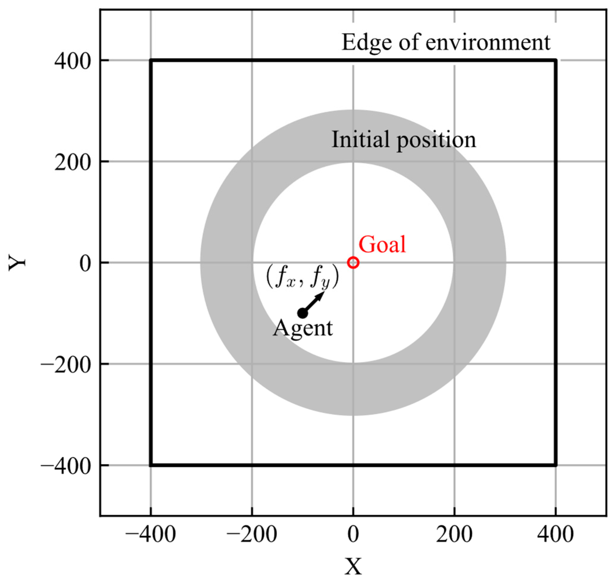
The task of the agent was to achieve the goal from its initial position. The goal $(x_{goal},y_{goal})$ is set at $\left(\mathrm{0,0}\right)$ and the initial position of the agent, $(x_{init},y_{init})$, is randomly set in an area described by Equation (7). The initial velocities $({v_x}_{init},{v_y}_{init})$ are $\left(\mathrm{0,0}\right)$. The area of the learning environment is given by Equation (8).

$$\left(x_{init},y_{init}\right)\in \left\{\left(x,y\right)|\left(200\le \sqrt{{\left(x_{goal}-x\right)}^2+{\left(y_{goal}-y\right)}^2}\le 300\right)\right\}$$

(7)

$$\left\{\left(x,y\right)|-400\le x\le 400,-400\le y\le 400\right\}$$

(8)

The motion of the agent is defined as the motion of a mass point, considering the resistance corresponding to the velocity. The equations of motion are described by Equation (9), where $m$, $f$, $\kappa$ are mass and force for each axis, and gain of resistance, respectively. The values of mass and resistance gain were set to 10 and 2, respectively.

$$\left\{\begin{array}{c}m{\displaystyle \frac{d^{2}x}{d{t}^2}}=f_x-\kappa {\displaystyle \frac{dx}{dt}}\\ m{\displaystyle \frac{d^{2}y}{d{t}^2}}=f_y-\kappa {\displaystyle \frac{dy}{dt}}\end{array}\right.$$

(9)

As the action space of the DQN is defined in a discrete space, the actions of the AI are set as discrete forces, $F$. The action options are the nine forces described in Equation (10).

$$F=\left({\displaystyle \genfrac{}{}{0pt}{}{f_x}{f_y}}\right)≔\left\{\left({\displaystyle \genfrac{}{}{0pt}{}{fsin\left(\theta \right)}{fcos\left(\theta \right)}}\right)|\left(f=0\right)\vee \left(f=10\wedge \theta \in \left\{0,{\displaystyle \frac{\pi }{4}},{\displaystyle \frac{\pi }{2}},\dots ,{\displaystyle \frac{7\pi }{4}}\right\}\right)\right\}$$

(10)

The schematic view of the learning environment is shown in Figure 1. The number of steps in one episode was 240, and the time step was set to 1. The agent makes decisions at each time step. The conditions for ending the episode are as follows: 240 steps are performed, the distance between the agent and goal becomes less than 10, or the agent exits the learning environment.

3.2. Design of Reward

Because the agent determines the goodness of an action using a reward, a reward appropriate to the task should be designed. To achieve an action to reach a goal from a randomly given initial position, a reward is given according to the deviation from the goal, $r_t^{dev}$. The agent gets a higher reward by being closer to the goal. Furthermore, the reward, according to the changes in the distance between the agent and the goal, $r_t^{dec}$, is given if the distance decreases. The $r_t^{dec}$ is affected by the agent’s action rather than by $r_t^{dev}$. Therefore, $r_t^{dec}$ clarifies the goodness of the action. Finally, a large negative reward was provided if the agent exited the environment. The rewards and total reward were calculated using Equations (11)–(14), where $d_t$ is the distance between the agent and goal.

$$r_t^{dev}=-{\displaystyle \frac{d_t}{400\sqrt{2}}}-0.1$$

(11)

$$r_t^{dec}=0.03+0.07\ast \left|1-\arccos \left({\displaystyle \frac{d_{t+1}-d_t}{\sqrt{v_x^2+v_y^2}}}\right)/(\pi /2)\right|$$

(12)

$$r_t^{done}=\left\{\begin{array}{l}-10,iftheagentgoout\\ 0,else\end{array}\right.$$

(13)

$$r_t=\left\{\begin{array}{c}{r}_t^{dev}+r_t^{done},d_{t+1}>d_t\\ r_t^{dev}+r_t^{dec}+r_t^{done},d_{t+1}\le d_t\end{array}\right.$$

(14)

The learning task can also be completed by simply giving a large, positive reward when the agent reaches the goal. However, such sparse reward settings for agents’ states destabilizes the learning process. An auxiliary reward indicating the goodness of an agent’s action is helpful for stable learning. Therefore, the reward depending on an agent’s state, described in Equation (11), and the reward depending on the agent’s action, described in Equation (12), were used in tandem.

3.3. Design of Observation

The observation is the input data for the neural network and should include sufficient data to predict the reward. In this study, the observed state is defined by Equation (15), where $(dx,dy)$ and $(v_x,v_y)$ are the relative positions of the goal and the velocities of the agent, respectively. These values are scaled from −1 to 1. The input data for the neural network were the current state and the states in the previous four steps.

$$s_t≔\left[v_x/5,v_y/5,dx/800,dy/800\right]$$

(15)

4. Reliability Quantification

4.1. Applicability of Random Network Distillation

In RND, an intrinsic reward is provided when an agent experiences an unknown state, and exploration of the unknown state is encouraged. Thus, the value of the intrinsic reward was used as the value of inadequacy to the state, and RND was used for reliability evaluation. A neural network consists of multiple layers, and features are extracted from each layer. Because the output of each layer may be changed significantly by smaller changes in the input data it cannot be possible to extract similar features from similar states. Thus, an uncertainty evaluation for extracted features is more appropriate than one for the input data. Therefore, the uncertainty of the features extracted before the last hidden layer was evaluated. The structure of the neural network is defined according to RND, as shown in Figure 2. The neural network comprises two parts: a DQN network and an RND network that evaluates the uncertainty of the extracted features. The DQN network consists of five fully connected layers (FC). The numbers of nodes in these layers are 256, 256, 128, 128, and 9, respectively. The activation functions in the DQN are the ReLU function in the hidden layers and the linear function in the output layer. The target network and predictor network consist of five FCs, with their numbers of nodes being 512, 512, 256, 128, and 15, respectively. The activation functions in the hidden layers of the RND networks and output layers are a softsign function and linear function. Any DRL method can be applied by setting up a neural network instead of a DQN.

During training, the parameters of the neural networks that evaluate uncertainty are updated to minimize the output values. The parameters of the neural network predicting the Q values were updated to minimize the loss function of the DQN. To ensure that reliability quantification does not affect the DRLs, these updated processes are independent. The training hyperparameters are listed in

Table 1. Hyperparameters for training.

Parameter	Value
Learning steps	20,000,000 [steps]
Batch size	1024
Learning rate	0.001
Target model update	0.01
Optimizer	Adam
L1 regularization	0.0001

.

After training until the loss values converged, the trained model was evaluated in the simulation by varying the initial position within the ranges shown in Equation (16). To evaluate the action of the agent and the uncertainty of the learning environment, the ranges were wider than those in the learning environment, and the episode did not end if the agent exited the learning environment.

$$\left({\mathit{x}}_{\mathit{e}\mathit{v}\mathit{a}\mathit{l}\mathit{u}},{\mathit{y}}_{\mathit{e}\mathit{v}\mathit{a}\mathit{l}\mathit{u}}\right)\in \left\{\left(\mathit{x},\mathit{y}\right)|{\displaystyle \genfrac{}{}{0pt}{}{\mathit{x}\in \left\{\mathbf{-}\mathbf{700},\mathbf{-}\mathbf{630},\dots ,\mathbf{630},\mathbf{700}\right\}}{\mathit{y}\in \left\{\mathbf{-}\mathbf{700},\mathbf{-}\mathbf{630},\dots ,\mathbf{630},\mathbf{700}\right\}}}\right\}$$

(16)

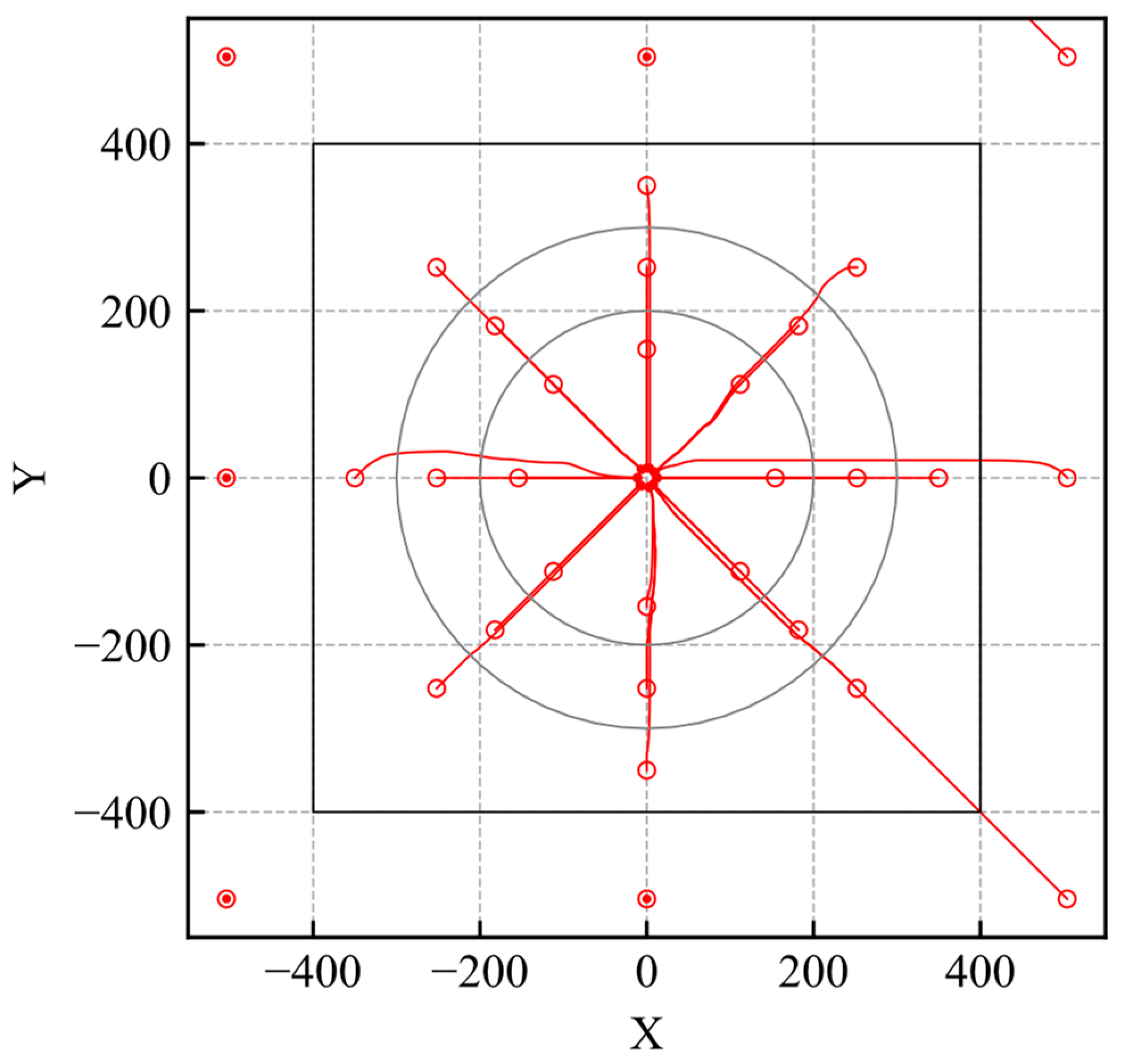
The evaluation trajectories are shown in Figure 3. The unfilled and filled red markers indicate the agent’s initial and last positions, respectively, and the shade of color indicates the time history. As shown in Figure 3, the agent can reach the goal regardless of where the initial position is set within the learning environment. If the initial position is set outside the environment the agent cannot reach the goal.

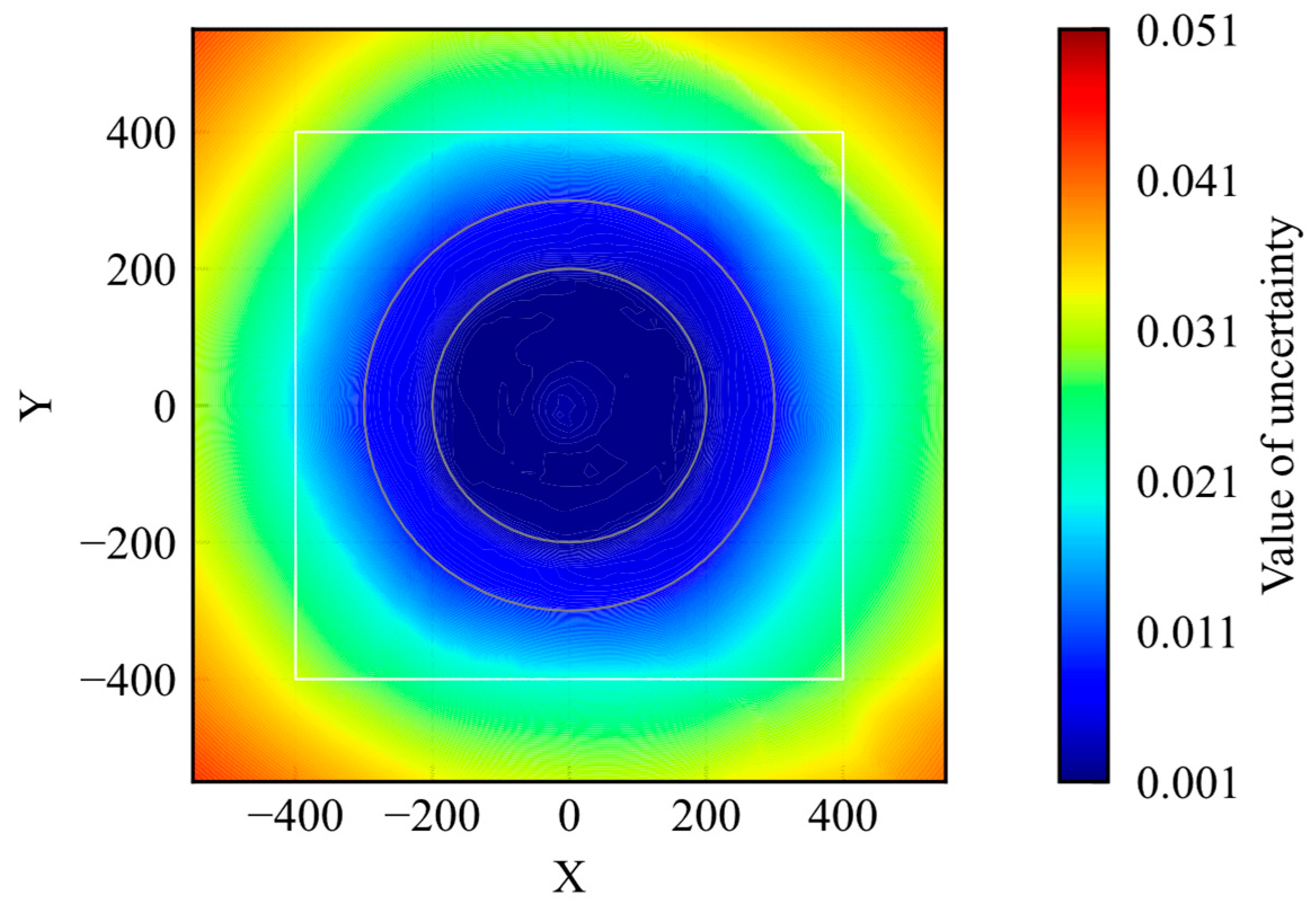
Figure 4 shows the distribution of the uncertainty. The figure shows the average uncertainty values when the agent passed through the points. During the training process, the agent acted randomly in the early steps and experienced a wide range of states in the environment. At the end stage of training, the agent moves to the given goal from its initial point on the shortest course. Thus, the number of states experienced inside the initial position, inside the learning environment, and outside the learning environment decreased in that order. According to Figure 4, the value of uncertainty regarding the extracted features decreases with the distance to the goal. This result is appropriate for the number of experiences. To compare the uncertainty distribution of the trained model with that of the untrained model, the uncertainty distribution of the untrained model is shown in Figure 5. The uncertainty values were lower in some areas of the model distribution before training. Because the untrained model did not learn any states, the uncertainty value should be higher. Nevertheless, the maximum value was smaller than that of the trained model. It is obviously not appropriate for the uncertainty quantification.

Based on the results shown in Figure 4 and Figure 5, the possibility of applying RND to uncertainty quantification is shown; however, there are two issues regarding the application of RND to evaluate uncertainty. First, RND does not ensure that the value of uncertainty is large in an unknown state, as shown in Figure 5. Second, the uncertainty range depends on the initial parameters. If the maximum and minimum values differ according to the model, it is difficult to set a criterion to determine whether the model is in a well-trained state. These issues were caused by the value differences in the output of the target network, and the predictor network depended on the initial parameters. From the perspective of evaluation, it is important to ensure that the value of uncertainty is small in well-known states and large in unknown states and that the range of uncertainty is constant. If this is not ensured, the uncertainty coincidentally decreases for unknown states. Therefore, it is not preferable to use RND as an evaluation method.

4.2. Reliability Quantification Method

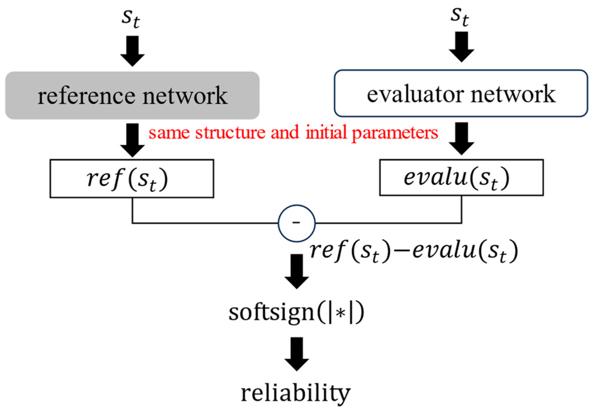
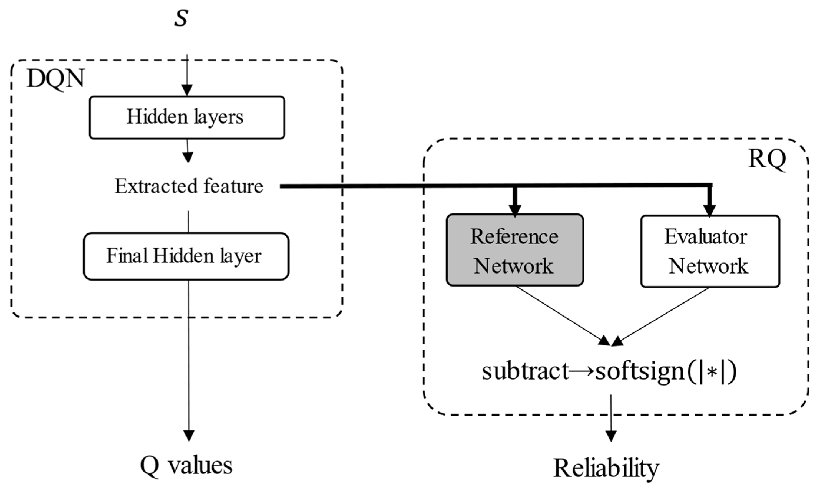
In the previous section, issues related to the application of RND to uncertainty evaluation were addressed. Thus, an improved method suitable for evaluating reliability was proposed. To evaluate reliability, two networks, a reference network, and an evaluator network, were used. Reliability was obtained by calculating the absolute error between the reference and evaluator networks, and a softsign function was applied to the absolute error to scale a range from 0 to 1. The reliability value was calculated using Equation (17), and the calculation flow of the reliability is shown in Figure 6.

$$Reliability\left(s\right)=\mathrm{s}\mathrm{o}\mathrm{f}\mathrm{t}\mathrm{s}\mathrm{i}\mathrm{g}\mathrm{n}\left(\left|Ref\left(s|{\theta }_r\right)-Evalu\left(s|{\theta }_e\right)\right|\right)$$

(17)

The scheme is similar to that of RND, but there are some differences. In RND, the target and predictor networks can have different structures, and their initial parameters are determined randomly; however, the reference and evaluator networks should have the same structure and initial parameters. Because the reference and evaluator networks are the same neural networks before training, their outputs are the same if the same input date is provided. This ensured that the reliability value reached zero before training. During the training process, the parameters of the reference network were fixed, and those of the evaluator network were updated to maximize the reliability value. 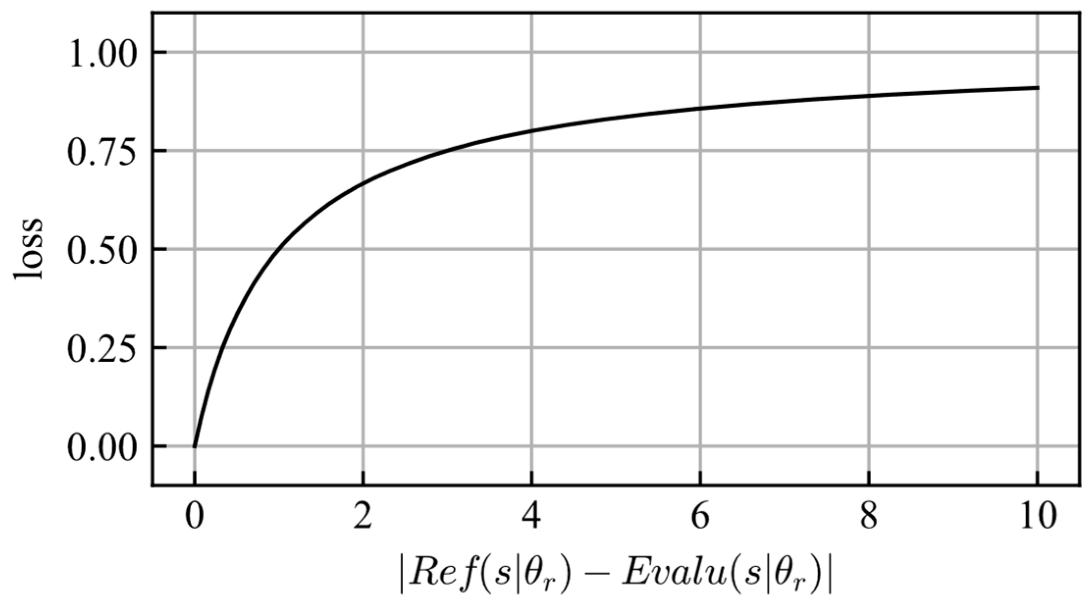Thus, the loss function can be described using Equation (18), where $Ref\left(s|{\theta }_r\right)$, $Evalu\left(s|{\theta }_e\right)$, ${\theta }_r$, and ${\theta }_e$ are the reference network, the evaluator network, the parameters of the reference network, and the parameters of the evaluator network, respectively. The shape of the loss function is shown in Figure 7.

$$Los{s}_{improve}\left({\theta }_e\right)=\mathbb{E}\left[-\mathrm{s}\mathrm{o}\mathrm{f}\mathrm{t}\mathrm{s}\mathrm{i}\mathrm{g}\mathrm{n}\left(\left|Ref\left(s|{\theta }_r\right)-Evalu\left(s|{\theta }_e\right)\right|\right)\right]$$

(18)

The gradient of the loss function decreased as reliability increased. Therefore, the larger the reliability value, the more difficult it is to change. This means that sufficiently trained experience fades slowly and is similar to human memory.

Furthermore, because the trained model is largely affected by recent training data, the reliability of past trained situations should decrease step by step. In this regard, the parameters of the evaluation network were updated to minimize the reliability of irrelevant training data, $S_{irr}$, and irrelevant data were generated randomly. The loss function that considers the forgetting experience is described by Equation (19), where $s_{irr}$ is a randomly generated irrelevant state.

$$Los{s}_{forget}\left({\theta }_e\right)=\mathbb{E}\left[\mathrm{s}\mathrm{o}\mathrm{f}\mathrm{t}\mathrm{s}\mathrm{i}\mathrm{g}\mathrm{n}\left(\left|Ref\left(s_{irr}|{\theta }_r\right)-Evalu\left(s_{irr}|{\theta }_e\right)\right|\right)\right]$$

(19)

Finally, the loss function for reliability quantification is described as Equation (20).

$$Los{s}_{reliability}\left({\theta }_e\right)=Los{s}_{improve}\left({\theta }_e\right)+Los{s}_{forget}\left({\theta }_e\right)$$

(20)

The regularization term used to prevent overtraining is defined in Equation (21), where $p$ and $\lambda$ are a dimension and a power of regularization, respectively. This restricted the distance of the parameters between the evaluation and reference networks.

$$\lambda {\displaystyle \frac{1}{p}}{\left|{\theta }_e-{\theta }_r\right|}^p$$

(21)

4.3. Reliability Quantification for DQN-Based Control

To validate the proposed method, it was evaluated in the same manner as that described in Section 4.1. Here, the DQN is applied to train a model. The structure of the neural network for the proposed reliability quantification is shown in Figure 8. The hyperparameters for training are the same as those listed in Table 1.

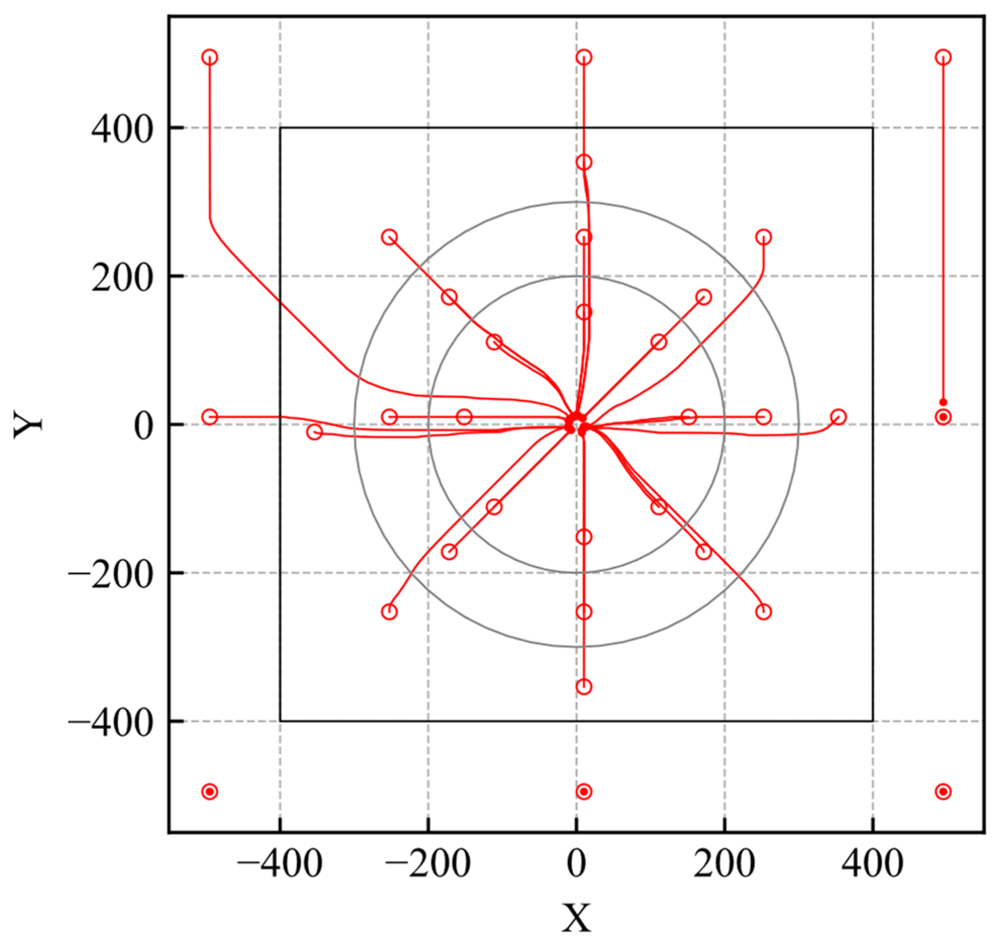
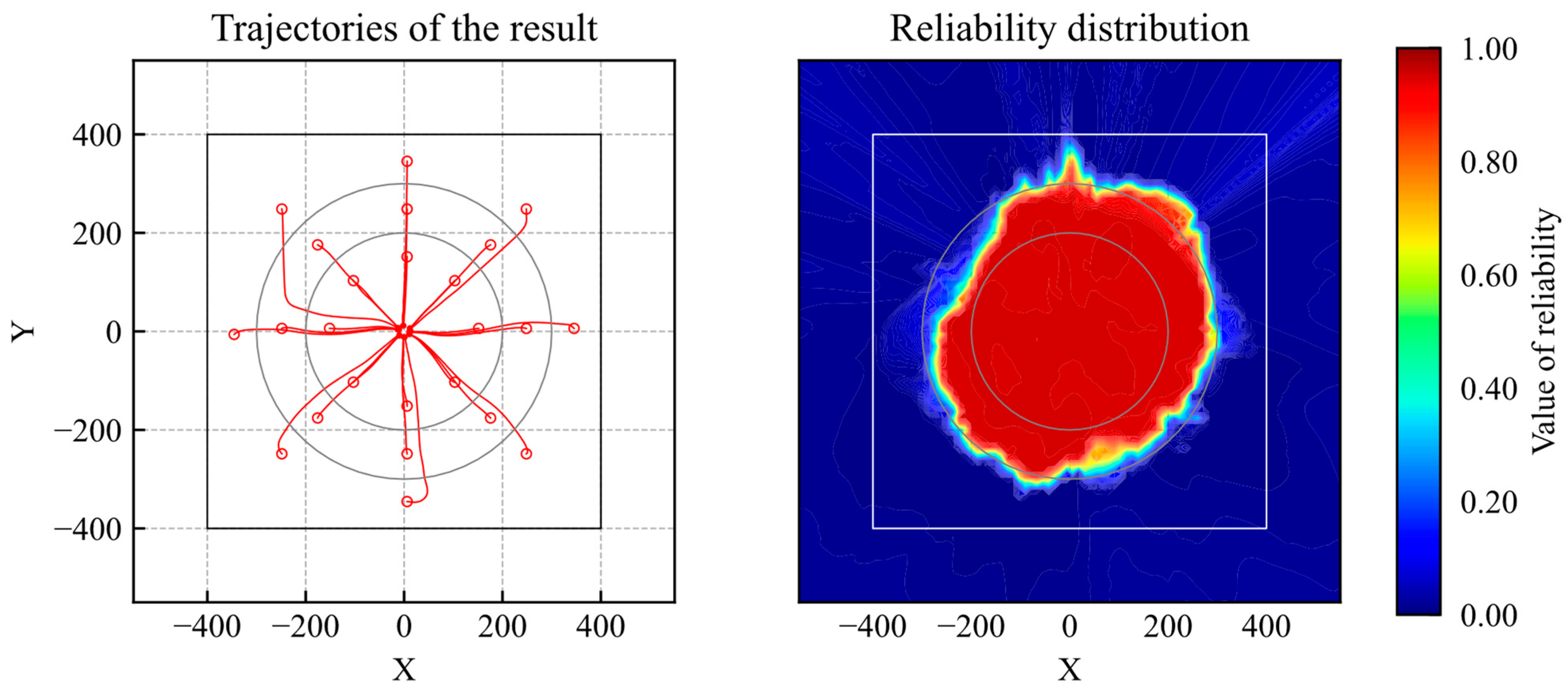
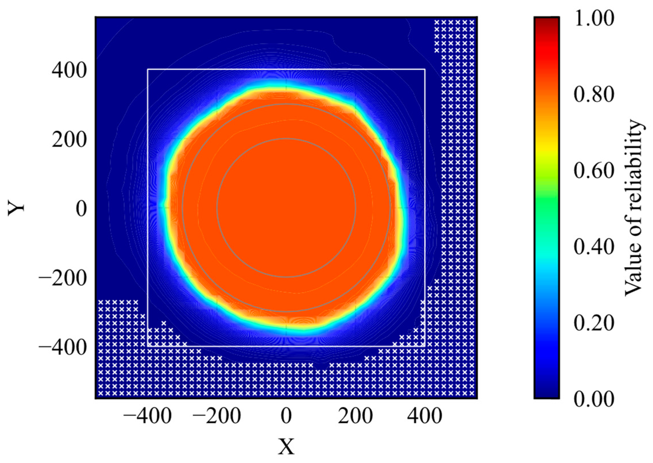
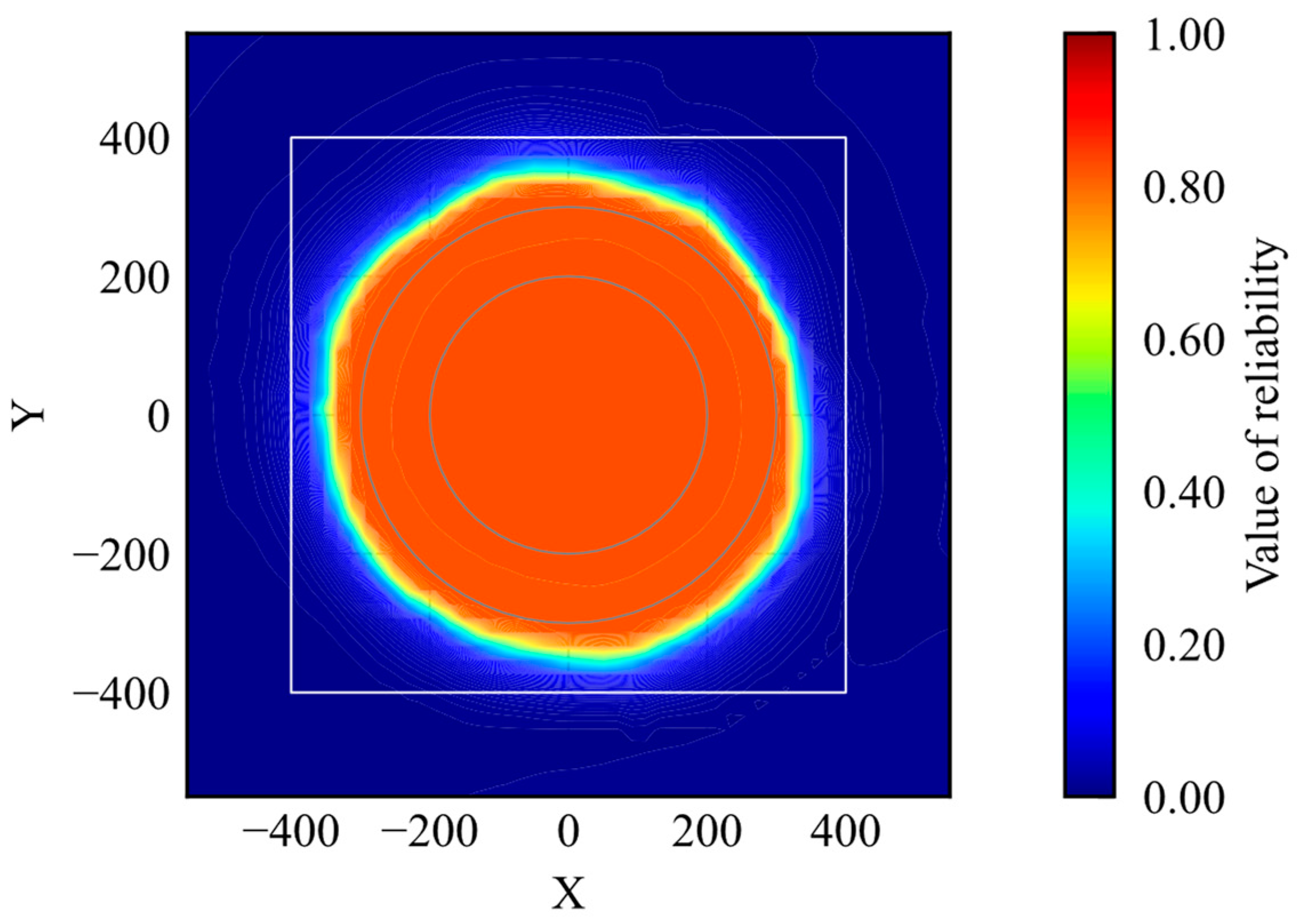
The simulation trajectories are shown in Figure 9. As shown in Figure 9, the agent learns the optimal action within the learning environment. The reliability distribution is shown in Figure 10. According to Figure 10, the reliability becomes high within the range of the initial positions. According to the results, the proposed method can evaluate whether the agent is trained.

4.4. Reliability Quantification for DDPG-Based Control

The proposed algorithm was validated by applying DDPG to train a model. DDPG is a representative method of actor–critic DRL. Because DDPG deals with a continuous action space, an action of the agent was changed from discrete forces, given in Equation (10), to a direction of force, shown in Equation (22), where ${\theta }_{DDPG}$ is an action of the agent on DDPG and its range is from 0 to $2\pi$.

$$F=\left({\displaystyle \genfrac{}{}{0pt}{}{f_x}{f_y}}\right)≔\left({\displaystyle \genfrac{}{}{0pt}{}{f\mathrm{s}\mathrm{i}\mathrm{n}\left({\theta }_{DDPG}\right)}{f\mathrm{c}\mathrm{o}\mathrm{s}\left({\theta }_{DDPG}\right)}}\right)$$

(22)

DDPG learns an optimal action using an actor network and a critic network. The structures of the actor and critic networks incorporating reliability quantification are shown in Figure 11. The reliabilities of the actor and critic networks are evaluated by quantifying the reliability of features extracted before their final layers. The AI was trained in the same training environment described in Section 4.3.

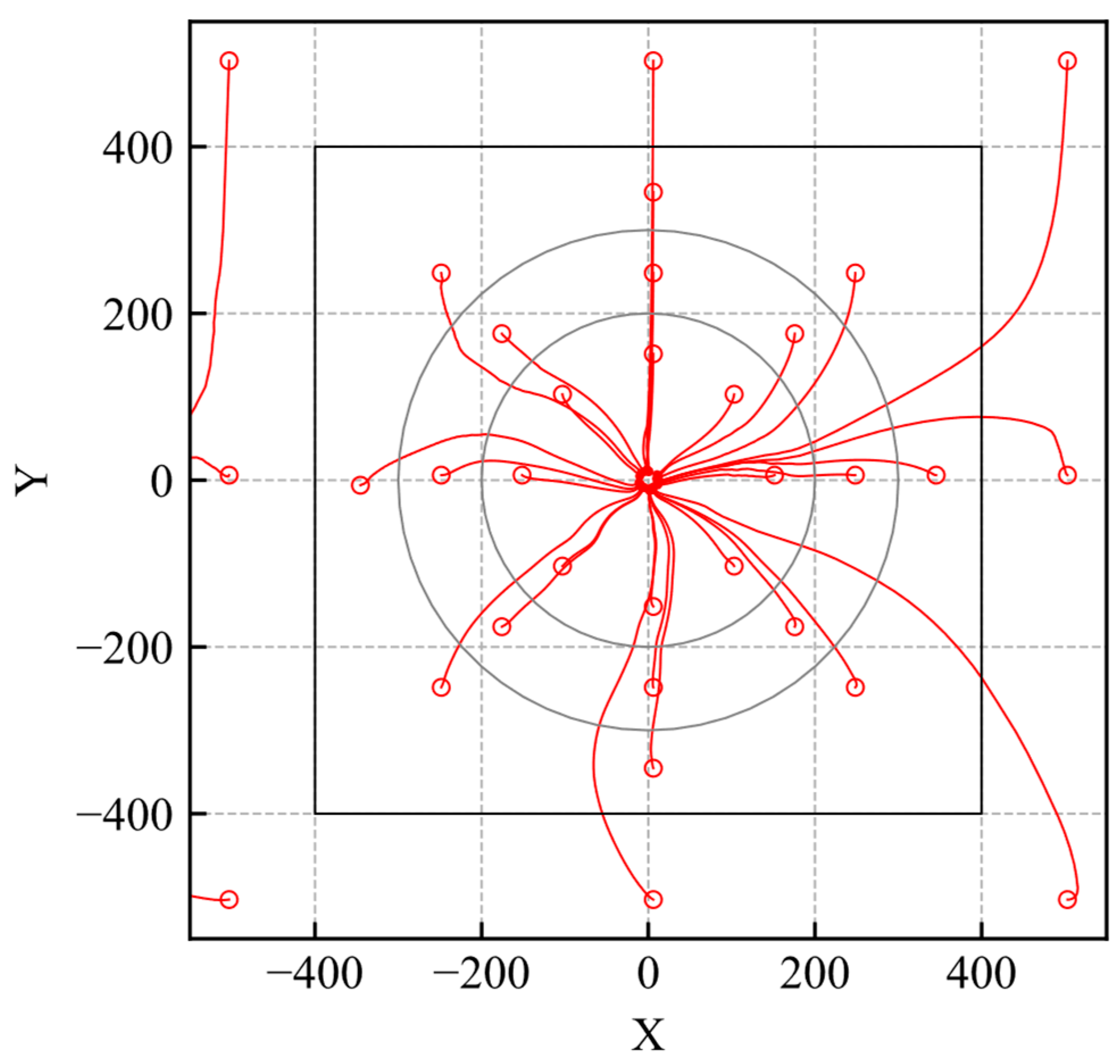
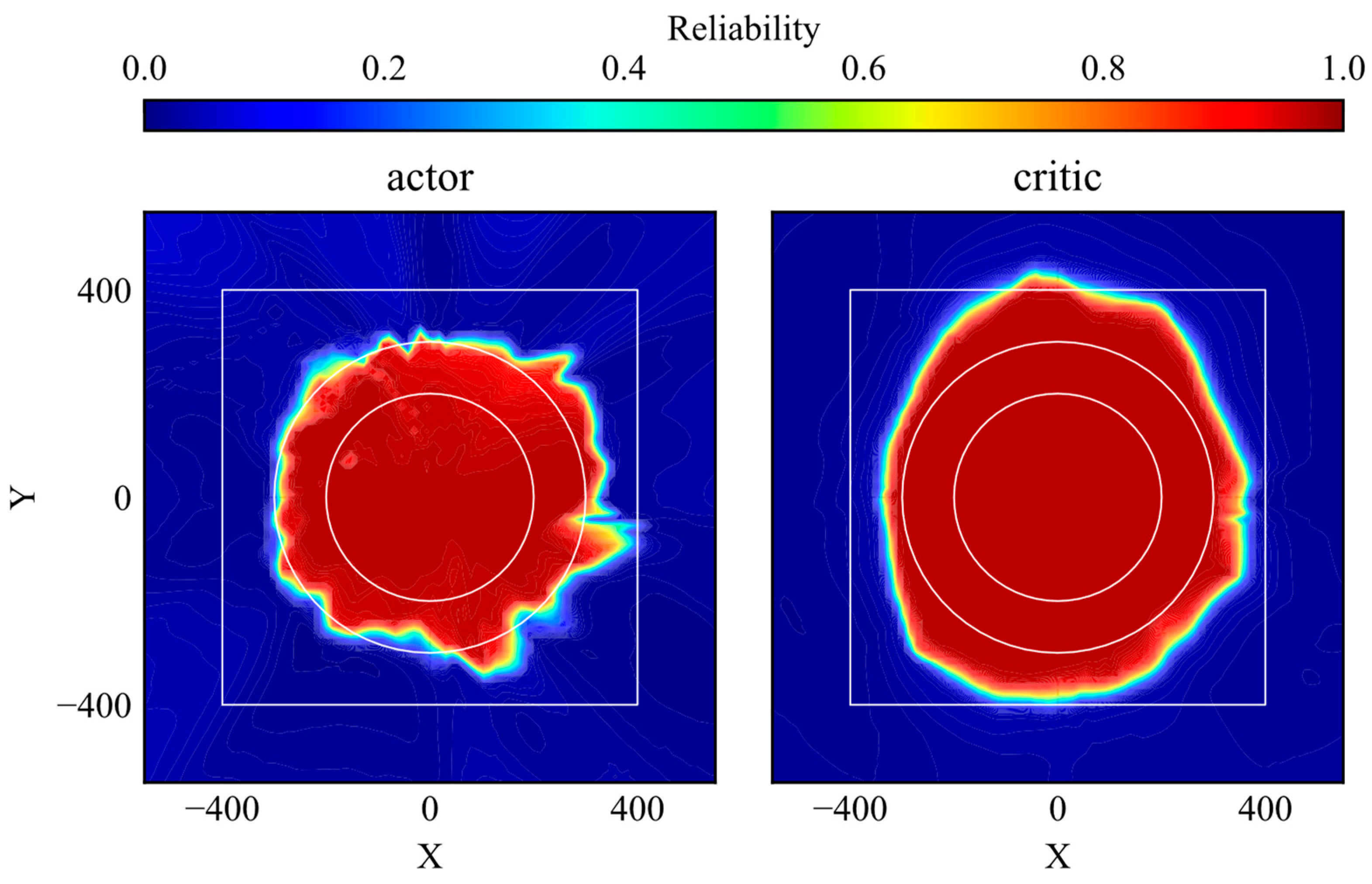
The simulation trajectories of the trained DDPG model are shown in Figure 12. The agent learns the optimal action within the learning environment. The reliability distributions of the actor and critic networks are shown in Figure 13. The reliability within the range of the initial position in the learning environment is high, as shown in Figure 13. Subsequently, the agent moves smoothly to the goal when its initial position is within that range, as shown in Figure 12. These results show similar trends to those for the DQN-based control presented in Figure 10. However, the range of high reliability is different from that of DQN-based control. First, the area of high reliability for DQN-based control almost matches the area of the initial position in the learning environment, while that of the critic network becomes wider. This indicates that the critic network can extract similar futures even if the state changes slightly. Second, the edge of the area with high reliability for the actor network is unclear compared to that for DQN-based control. This is caused by the difference in the learning objectives. Although both the critic network and the DQN learn the Q value, the actor network maximizes the output of the critic network, and, hence, the stability of learning of the critic network becomes worse compared to that of DQN. Although some differences can be found, as mentioned, the high reliability areas of the actor and critic networks clearly correspond to the area of the initial position in the learning environment. Therefore, it can be concluded that the proposed method for reliability quantification is applicable to representative DRL-based controls.

5. Discussion

5.1. Comparison with Random Network Distillation

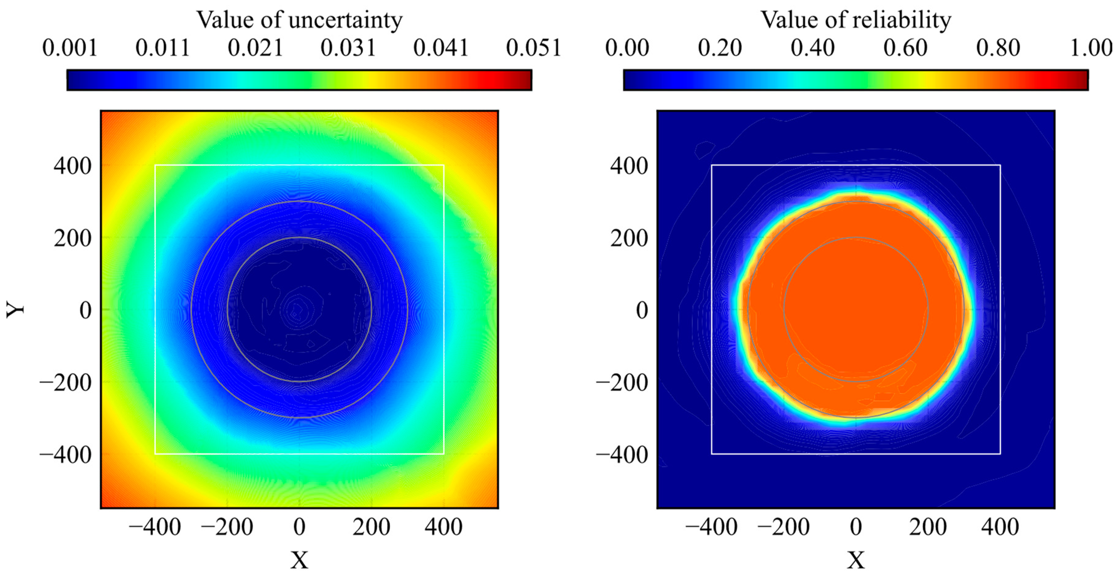
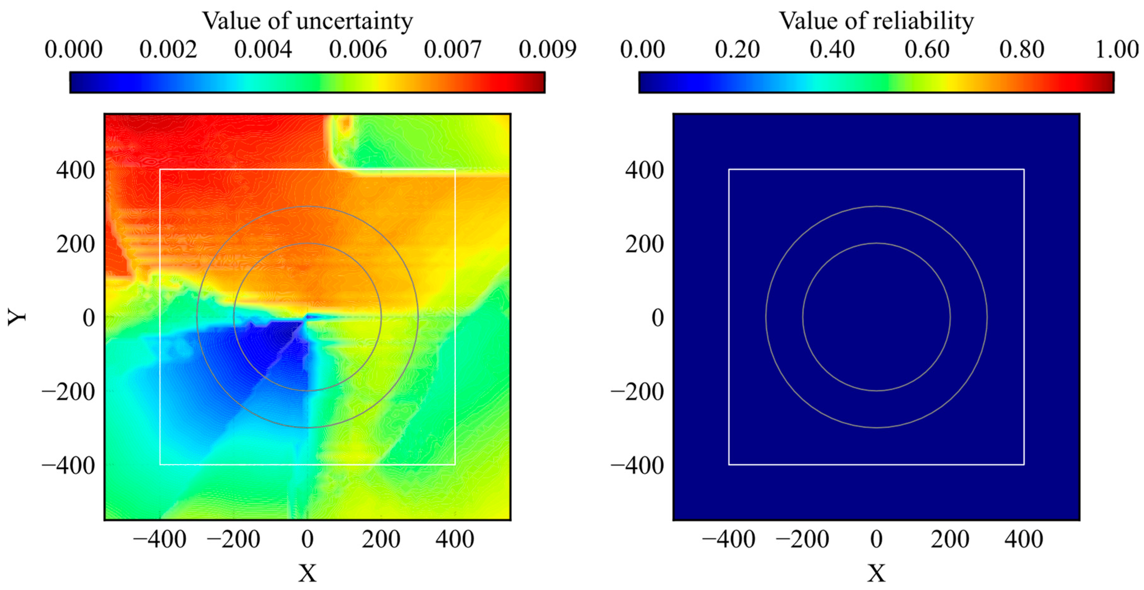
The proposed method was compared with uncertainty quantification using RND. The distributions of the trained and untrained models are presented in Figure 14 and Figure 15, respectively. Because reliability and uncertainty are opposite evaluation indexes, the value size has the opposite meaning.

According to the comparison results, the distribution clearly classifies the high-reliability and low-reliability areas rather than the uncertainty of RND. The range of the uncertainty distribution depends on the model parameters and structure in RND, whereas the range of the reliability distribution is fixed at 0–1 in the proposed method. Furthermore, as shown in Figure 15, the reliability of the untrained model was 0 for all the states. These two aspects are important for their use as evaluation methods.

5.2. Relationships between Reliability of AI and Feasibility on Task

The agent should reach the goal if an initial position is within the high-reliability area. The initial positions where the agent could not reach the goal are examined and shown by markers in Figure 16.

According to the result, the markers do not exist inside the high-reliability area. It indicates that the agent can achieve the task when the agent is initialized in a high-reliability state. Therefore, the proposed method is useful to quantify the reliability of DRL-based control.

6. Switching of Trained Model

It was demonstrated that the proposed method could evaluate the reliability of the trained model described in the previous section. The reliability value becomes 0 in the untrained state and 1 in the well-trained state. In RND, because the range of uncertainty depends on the model, a comparison of the uncertainty between models is not possible. The proposed method ensured that the reliability ranges were identical, enabling the reliability of the models to be compared. Therefore, the effectiveness of switching trained models was demonstrated as an application method. The quality of the sampled training data is a major issue in DRL. However, it is difficult to solve this problem completely. One solution is to switch between the trained models. Using several trained models, the untrained states of each model can cover each other. However, it is difficult to set criteria for switching models. As a solution, the reliability value can be used as a criterion for the switching model. Therefore, the effectiveness of switching models is discussed in this section.

Before demonstrating the switching models, four models with biased experiences were developed. The ranges of the initial positions were different for these models. The initial positions of the $i$-th model were determined randomly within the range expressed in Equation (23). The $i$-th model trained the states of the $i$-th quadrant. The reward and observations were the same as those described in the previous sections.

$$\left(x_{init}^i,y_{init}^i\right)\in \left\{\left(\mathrm{d}·\cos \left(\theta \right),d·\sin \left(\theta \right)\right)|{\displaystyle \genfrac{}{}{0pt}{}{200\le d\le 300}{\frac{\pi }{2}\left(i-1\right)\le \theta <\frac{\pi }{2}i}}\right\}(i=1,2,3,4)$$

(23)

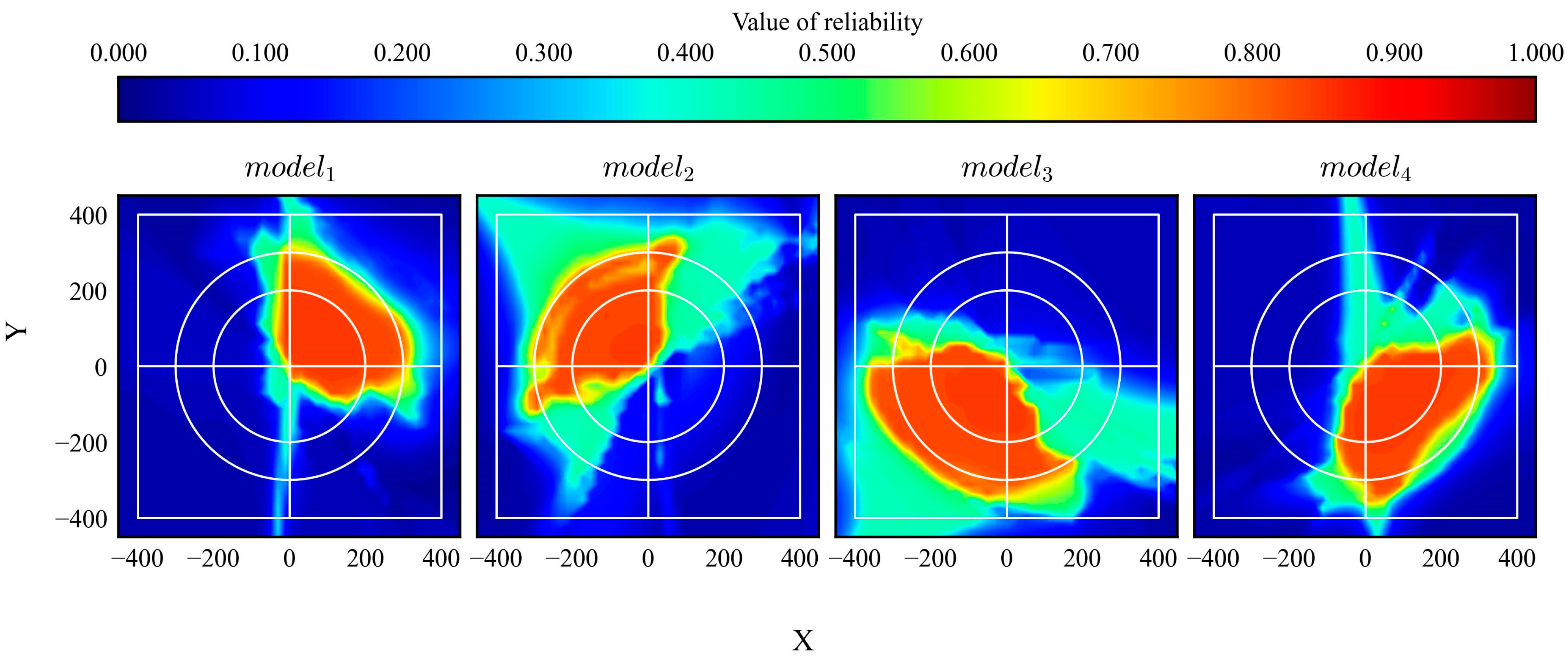
After training, all models were evaluated. The trajectories and distribution of the reliability are shown in Figure 17 and Figure 18, respectively. The gray area in Figure 17 indicates the range of the initial states. According to the results, the trained models achieved their goals and exhibited high reliability within their trained quadrants.

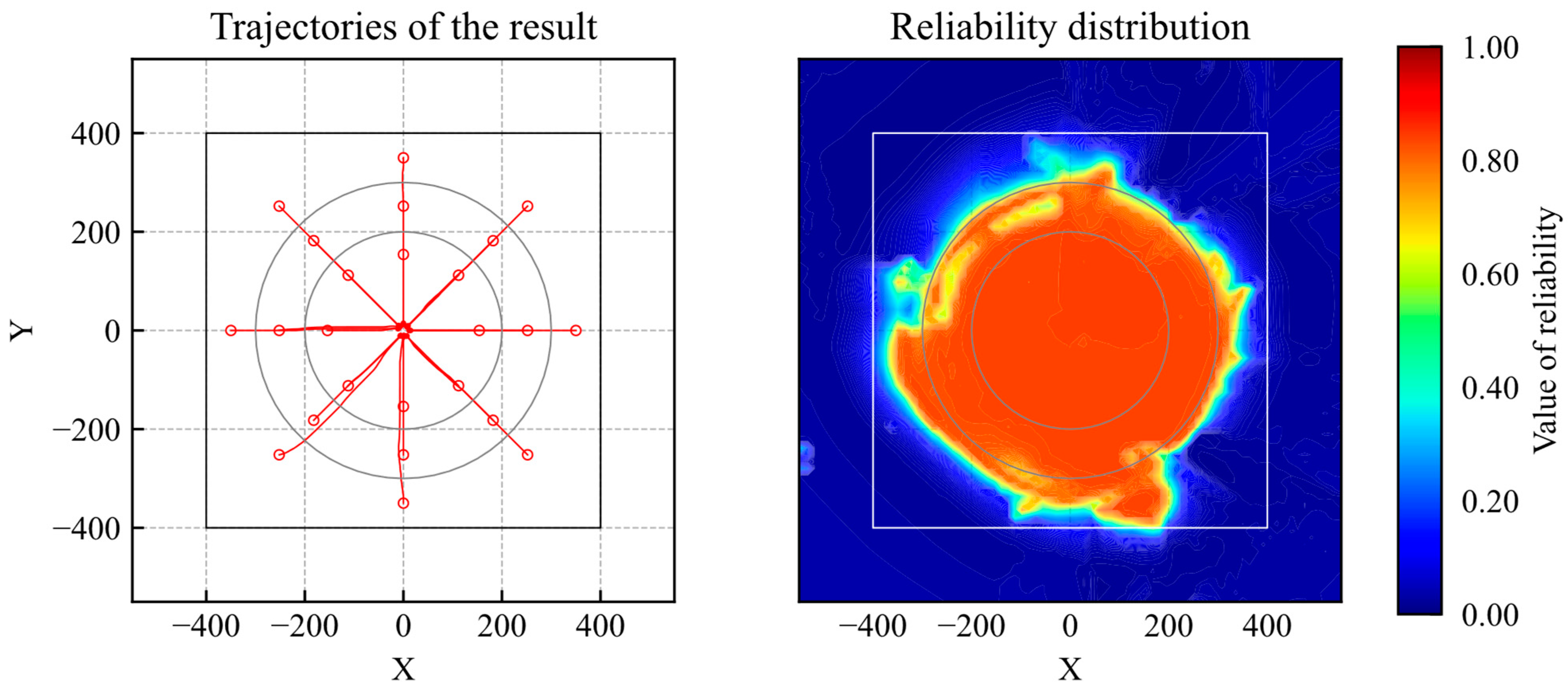
The trained models were then switched. In the simulation, the optimal actions and reliability values of all models were calculated at every time step. Then, the action of the agent with the maximum reliability was used as an action in the simulation. The results of the trajectories and reliability are shown in Figure 19. According to the evaluation results, the agent achieved the goal from all initial positions and exhibited high reliability over a wider area in the learning environment.

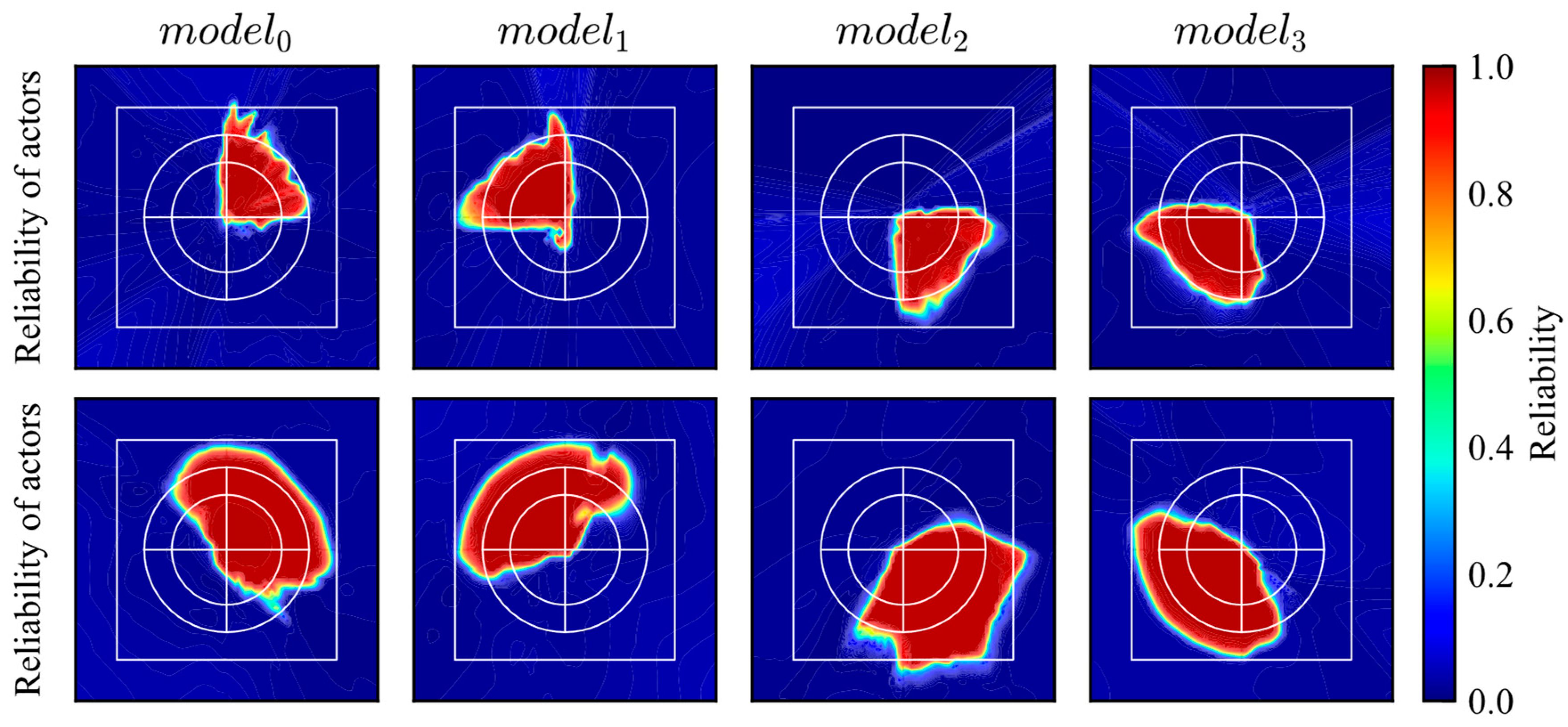
In addition, the effectiveness of the model switching was validated by applying it to a DDPG-based control. The trajectories and reliability distributions of the DDPG-trained model using biased experience are shown in Figure 20 and Figure 21. Then, the trajectories and reliability distribution of the switching models are shown in Figure 22. According to the evaluation results, the agent reached the goal from all initial positions and exhibited high reliability over a wider area.

Through the validation of trained model switching applied to DQN-based and DDPG-based controls, it can be concluded that the performance of DRL-based controls is improved by adopting the switching model technique according to the proposed reliability quantification method.

7. Conclusions

A major challenge of DRL is reliability quantification. It is necessary to evaluate the reliability in real time for the actual application of DRL-based control in safety-critical systems. In this study, the following was conducted to propose a novel method for reliability quantification of DRL-based control.

First, the applicability of an existing method, RND, for uncertainty evaluation was investigated. Uncertainty is defined as the opposite evaluation index of reliability. It was confirmed that the range of the uncertainty value depends on the initial parameters. Hence, it cannot be ensured that the uncertainty value increases in an unknown state. Because the range of uncertainty is not fixed and the uncertainty value often becomes small for untrained states, RND is difficult to use for uncertainty quantification. Second, a reliability quantification method was proposed to solve those problems. Reliability was evaluated by the difference between the reference and evaluator networks, which had the same structure and initial parameters. The parameters of the reference network were fixed, whereas those of the evaluator network were updated to maximize the difference in output between the two networks for the trained data and minimize the difference in output between them for the irrelevant data. The proposed method was validated for DQN-based and DDPG-based controls of a simple task. Consequently, it was confirmed that the proposed method can evaluate reliability and identify a well-trained domain in the learning environment. Finally, an example application was presented. To address the lack of experience in a trained model, switching the trained models according to their reliability was investigated. Using four models trained with biased experiences, it was demonstrated that a given task could be completed in any situation by switching models according to their reliability.

The advantages of the proposed method are that the range of values is fixed and that the value of reliability becomes zero in untrained situations and one in well-trained situations. These advantages are beneficial for evaluating reliability and creating a criterion easily. The proposed method can therefore be used in various applications, such as the switching of trained models. By switching some trained models using the reliability, the best trained model can be chosen in any situation. If an untrained situation is inputted to one of them, another one with a higher reliability can choose the optimal action instead. Hence, this method contributes to the resolution of the issue of biased experience in DRL models. In addition, this can improve the performance and robustness of DRL-based control. Another application example involves identifying operational design domains (ODDs) of the control. Additionally, the proposed method can calculate the intrinsic reward as opposed to RND.

In future studies, its applicability to an actual environment should be validated. In actual environments, the input state is affected by data noise. Its effects are not clear at this moment but are important for practical use. The proposed method assumes that the loss value converges, although it does not ensure that the loss value in all states converges to zero. Therefore, the convergence of the loss of the training process in reliability quantification should be considered.

References

- Vyas, A.; Jammalamadaka, N.; Zhu, X.; Das, D.; Kaul, B.; Willke, T.L. Out-of-distribution detection using an ensemble of self supervised leave-out classifiers. In Proceedings of the 15th European Conference on Computer Vision (ECCV), Munich, Germany, 8–14 September 2018; pp. 560–574. [Google Scholar] [CrossRef]
- Lindqvist, J.; Olmin, A.; Lindsten, F.; Svensson, L. A general framework for ensemble distribution distillation. In Proceedings of the 2020 IEEE 30th International Workshop on Machine Learning for Signal Processing (MLSP), Espoo, Finland, 21–24 September 2020. [Google Scholar] [CrossRef]
- Valdenegro-Toro, M. Sub-ensembles for fast uncertainty estimation in neural networks. In Proceedings of the 2023 IEEE/CVF International Conference on Computer Vision Workshops (ICCVW), Paris, France, 2–6 October 2023. [Google Scholar] [CrossRef]
- Pearce, T.; Brintrup, A.; Zaki, M.; Neely, A. High-quality prediction intervals for deep learning: A distribution-free, ensembled approach. In Proceedings of the 35th International Conference on Machine Learning, PMLR, Stockholm, Sweden, 10–15 July 2018; Volume 80, pp. 4075–4084. [Google Scholar]
- Wen, Y.; Tran, D.; Ba, J. Batch ensemble: An alternative approach to efficient ensemble and lifelong learning. In Proceedings of the 8th International Conference on Learning Representations, Addis Ababa, Ethiopia, 26–30 April 2020. [Google Scholar]
- Ashukha, A.; Lyzhov, A.; Molchanov, D.; Vetrov, D. Pitfalls of in-domain uncertainty estimation and ensembling in deep learning. In Proceedings of the 8th International Conference on Learning Representations, Addis Ababa, Ethiopia, 26–30 April 2020. [Google Scholar]
- Sedlmeier, A.; Gabir, T.; Phan, T.; Belzner, L.; Linnhoff, P.C. Uncertainty-based out-of-distribution classification in deep reinforcement learning. arXiv 2019. [Google Scholar] [CrossRef]
- Gawlikowski, J.; Saha, S.; Kruspe, A.; Zhu, X.X. Out-of-distribution detection in satellite image classification. In Proceedings of the RobustML Workshop at ICLR 2021, Virtual Event, 3–7 May 2021; pp. 1–5. [Google Scholar]
- Baier, L.; Schlor, T.; Schoffer, J.; Kuhl, N. Detecting concept drift with neural network model uncertainty. arXiv 2021. [Google Scholar] [CrossRef]
- Malinin, A.; Gales, M. Predictive uncertainty estimation via prior networks. In Proceedings of the 32nd International Conference on Neural Information Processing Systems, Advances in Neural Information Processing Systems. Montreal, QC, Canada, 3–8 December 2018; pp. 7047–7058. [Google Scholar]
- Amini, A.; Schwarting, W.; Soleimany, A.; Rus, D. Deep evidential regression. arXiv 2019. [Google Scholar] [CrossRef]
- Liang, S.; Li, Y.; Srikant, R. Enhancing the reliability of out-of-distribution image detection in neural networks. In Proceedings of the International Conference on Learning Representations 2018, Vancouver, BC, Canada, 30 April–3 May 2018. [Google Scholar]
- Hsu, Y.-C.; Shen, Y.; Jin, H.; Kira, Z. Generalized ODIN: Detecting out-of-distribution image without learning from out-of-distribution data. In Proceedings of the IEEE/CVF Conference on Computer Vision and Pattern Recognition 2020, Seattle, WA, USA, 13–19 June 2020; pp. 10951–10960. [Google Scholar]
- Osband, I.; Aslanides, J.; Cassirer, A. Randomized prior functions for deep reinforcement learning. arXiv 2018. [Google Scholar] [CrossRef]
- Burda, Y.; Edwards, H.; Storkey, A.; Klimov, O. Exploration by random network distillation. arXiv 2018. [Google Scholar] [CrossRef]
- Mnih, V.; Kavukcuoglu, K.; Silver, D.; Graves, A.; Antonoglou, I.; Wierstra, D.; Riedmiller, M. Playing Atari with deep reinforcement learning. arXiv 2013. [Google Scholar] [CrossRef]
- Lillicrap, T.P.; Hunt, J.J.; Pritzel, A.; Heess, N.; Erez, T.; Tassa, Y.; Silver, D.; Wierstra, D. Continuous control with deep reinforcement learning. In Proceedings of the 4th International Conference on Learning Representations (ICLR), San Juan, Puerto Rico, 2–4 May 2016. [Google Scholar]