A Computational Platform for Automatic Signal Processing for Bender Element Sensors ^†

Abstract

The small strain shear modulus is an important characteristic of geomaterials that can be measured experimentally using piezoelectric sensors (bender elements). However, most conventional signal interpretation techniques are based on the visual observation of the output signal and therefore inherently subjective. Objective techniques also exist, like the cross-correlation of the input and output signals, but they lack physical insight, as they rely on the (incorrect) assumption that input and output signals are similar. This paper presents GeoHyTE, the first objective and physically consistent toolbox for the automatic processing of the output signal of bender element sensors. GeoHyTE updates a finite element model of the experiment, iteratively searching for the small strain shear modulus that maximises the correlation between the experimental and numerical output signals. The method is objective, as the results do not depend on the experience of the user, and physically consistent, as the wave propagation process is modelled in full and signals of the same nature (output) are correlated. Moreover, GeoHyTE is nearly insensitive to grossly erroneous input by the user, both in terms of the starting point of the iterative maximisation process and refinement of the finite element model. The results obtained with GeoHyTE are validated against benchmark measurements reported in the literature and experimental data obtained by the authors. A detailed statistical analysis of the results obtained with GeoHyTE and conventional interpretation techniques is also presented.

1. Introduction

In geomechanics, the small strain shear modulus is an essential parameter for the dynamic characterisation of both cohesive and cohesionless geomaterials, and bender elements are one of the main techniques to measure it experimentally [1]. The use of bender elements as an alternative to the well-known resonant column test has been fuelled by their affordable price and flexible installation in various geotechnical testing devices. A ready-to-use bender element equipment costs tens of times less than a resonant column apparatus, and can be installed in oedometers [2], triaxial devices [3], and Rowe cells [4], among others. Field applications have also recently been reported [5]. On the other hand, bender elements induce unknown levels of (very small) strain in the geomaterial, so they can only be used to measure the shear modulus, not to relate it with the level of strain, as is the case of the resonant column. Moreover, the interpretation of the test is notoriously challenging and substantially depends on the experience of the analyst [6].

A typical experimental configuration consists of two bender elements, inserted on opposite sides of the sample: a transmitter whose lateral vibration (input signal) generates a transient shear wave, and a receiver which is triggered by the vibration of the material and generates the corresponding electrical signal (the output signal). The objective of the experiment is to use the information on the input and output signals to derive the shear modulus of the material [7]. This has mainly been achieved using two classes of interpretation techniques, namely time domain techniques and frequency domain techniques. Time domain approaches use pulse input signals and aim at either reading the arrival time of the shear wave directly from the output signal or obtaining it by cross-correlating input and output signals. From the travel time, the shear wave velocity is calculated, from which the small strain shear modulus is found by using a well-known equation of the Theory of Elasticity [8] (from this point on, the term shear modulus is used instead of small strain shear modulus, to keep the presentation simple). Conversely, frequency domain approaches generally use continuous harmonic input signals and measure the wavelength as a function of the input frequency from which the wave velocity is calculated [9]. Hybrid methods have also been reported [10]. Both time and frequency domain interpretation methods rely on the assumption that input and output signals are similar. This is not the case, however, as the output signal is strongly affected by the dispersion of the travelling waves, boundary reflection and radiation [11], as well as by the pollution of the main (shear) wave with secondary (compression) waves, byproducts of the lateral motion of the transmitter. For this reason, the peak on the output signal that marks the arrival of the shear wave may not be the first nor the highest local maximum, so its accurate identification using conventional time domain methods may be quite arduous. On the other hand, frequency domain methods assume that the wavelength is constant throughout the sample, which is generally not true due to wave distortion. These issues induce considerable subjectivity in the interpretation of the output signal, which is notoriously uncertain [6].

Between 2003 and 2006, an International Parallel Test took place in 23 geotechnical laboratories from 11 countries to test the consistency of the shear modulus measurements of the same samples of Toyoura sand. The specimens were tested under different state conditions (saturation, consolidation patterns, confining pressures). The results are known as one of the most convincing displays of uncertainty of the bender element predictions published to date [12]. The consistency of the results was particularly problematic for low confining pressures (50 kPa). For instance, for isotropically consolidated specimens, the standard deviation of the readings was larger than half of their average value, with measurements ranging from 25 MPa to 140 MPa.

Such findings highlight the need for consistency and objectivity in bender element tests, both in respect to the experimental setup and to the interpretation of the output signal. A standardisation effort was made in 2019, with the publication of the ASTM D8295-19 standard [13]. However, the standard only specifically addresses the triaxial setup (although the procedure can be extended to other geotechnical testing devices), and two time domain interpretation techniques, both based on the direct observation of the output signal. Therefore, their application is subjective and requires experienced analysts.

In 2016, a new, coupled numerical–experimental paradigm was proposed by the authors to improve the experimental setup and enhance the quality and objectivity of the interpretation of the output signal. Numerical models taking into account the multi-phase nature of geomaterials are used to describe in detail the wave propagation patterns and endorse the clear identification of the arrival time. The demonstration of the capacity of the numerical model to accurately recover the output signal obtained in the laboratory [14], even in two dimensions, was followed by the development of a mathematical framework for the automatic extraction of the shear modulus based on a fixed point model updating technique [15] and the optimisation of the experimental setup using the information gathered from the numerical models.

Conventional numerical modelling of piezoelectric testing is hindered by the high frequency of the input signal and the complexity of material behaviour. For this reason, the numerical models that fuelled the coupled, numerical and experimental paradigm were based on hybrid-Trefftz finite elements. These elements belong to a wider family of (non-conventional) hybrid finite elements [16] and are ideally suited for modelling high-frequency wave propagation. Unlike conform displacement elements, hybrid-Trefftz elements use domain approximations that satisfy the differential equation governing the problem. Consequently, they are frequency-insensitive and distinguish naturally between the various types of waves that enter the dynamic response of the sample. On the other hand, hybrid-Trefftz finite elements are very rare in public or commercial software [17,18]. Therefore, there is a need for public and user-friendly computational tools based on hybrid-Trefftz finite elements to bring the advantages of the new numerical–experimental approach to the fingertips of researchers and practitioners worldwide.

This paper reports on the novel computational platform GeoHyTE, a user-friendly toolbox for the automatic extraction of the shear modulus from the output signal of bender element sensors. GeoHyTE implements the fixed-point model updating technique reported in reference [15], its computations powered by hybrid-Trefftz elements for porous elastodynamics. GeoHyTE is the first and currently the only automatic and physically consistent interpretation toolbox for bender element experiments. The beta version of GeoHyTE was recently released at the International Conference “Trends on Construction in the Post-Digital Era” [19] and can be downloaded upon request [20].

Besides the presentation of GeoHyTE, the paper is aimed to coin model updating techniques for shear modulus extraction as a mainstream class of interpretation methods, along with the time and frequency domain methods. The study of the mathematical properties of the updating function demonstrates its excellent convergent properties and is a theoretical novelty in respect to reference [15]. Considering two particularly problematic testing configurations reported in the International Parallel Test [12], the paper compares the shear moduli obtained using a wide range of time and frequency domain interpretation methods with those predicted by GeoHyTE and check the latter for consistency. The robustness of the GeoHyTE predictions to sub-optimal user input (in terms of the initial estimation of the arrival time and coarse refinement of the numerical model) is also assessed.

The main advantage of the GeoHyTE platform is that it provides shear modulus estimates that are, at the same time, objective and physically consistent. The objectivity comes from the minimal user intervention required for the interpretation of the output signal, and means that multiple users obtain the same shear modulus prediction. The physical consistency lays in the use of numerical models especially tailored for the problem that is being solved, taking into account the multi-phase nature of geomaterials.

2. Conventional Interpretation Techniques for Bender Element Tests

Conventional interpretation techniques analyse the output signal of bender element tests to extract the travel time of the shear wave from the transmitter to the receiver. The travel time enables the calculation of the shear modulus, typically using the continuum elasticity expression,

$$\begin{array}{c}\hfill G_0=\rho \times {\left(v_S\right)}^2=\rho \times {\left(\frac{h}{t}\right)}^2\end{array}$$

(1)

where $G_0$ is the shear modulus, $v_S$ is the shear wave velocity, $\rho$ is the density of the material, h is the effective travel distance of the wave, typically (but not always) measured between the tips of the emitter and receiver bender elements, and t is the travel time that the wave required to cover this distance.

Measuring the travel time of the shear wave is the most complex issue, as its arrival at the receiver is often concealed by polluting compression waves. Various methods for measuring the travel time have been proposed to overcome this problem, but considerable disagreement still exists regarding the interpretation technique that would give the most accurate results [8,9,15,21,22,23,24,25,26]. Five time domain methods and one frequency domain method are used to validate the GeoHyTE measurements in Section 4.2. These methods are succinctly described below, for reader’s convenience.

2.1. Time Domain Methods

Time domain methods attempt to read the arrival time of the shear wave by analysing input and output signals directly. Figure 1 shows an example of a typical pulse input signal and an idealised received (output) signal.

Based on the idealised output signal presented in Figure 1, four classes of interpretation techniques are proposed, namely the first arrival method, the peak-to-peak method, the second arrival method, and the cross-correlation method. All are based on the assumption of a plane shear wave-front travelling through the sample in the absence of any reflected or refracted waves [8].

2.1.1. First Arrival of the Shear Wave

The estimation of the travel time was first performed by the direct visual identification of the arrival of the shear wave on the output signal. This technique was first introduced in geophysical field testing in [27] and was then adopted in geotechnical laboratories [21,22,25,26]. While points C (sometimes called first sharp, which is the designation adopted in this paper), D (first bump), or E (zero crossing) in Figure 1 are all good candidates for the shear wave arrival [12,28], Arulnathan et al. [8] showed that determining which of them is the actual arrival time is not straightforward. Moreover, traces of compression waves tend to pollute the readings and blur the exact location of the first arrival, introducing subjectivity into the technique [15].

2.1.2. Travel Time between Peaks of Input and Output Signals

The ‘peak-to-peak’ method is based on the assumption that the output signal bears high similarity to the input signal. The time lapse between the peak of the input signal (point B in Figure 1) and the first major peak in the output signal (point F) is taken as the travel time of the shear wave [26]. This method is very simple and popular, and it has been adopted by many researchers [8,12]. However, the identification of the first major peak may be difficult, since the output signal may have several consecutive peaks of similar amplitudes.

2.1.3. Second Arrival of the Output Wave

In order to minimise the uncertainty in the definition of the arrival time, a method based on the second arrival of the shear wave was reported in reference [8]. After the first passage through the receiver, the shear wave travels back to the transmitter and is reflected to the receiver for a second time. The time elapsed between the first and the second arrivals at the receiver is equal to twice the travel time of the wave between the two extremities of the sample [8]. This method solves uncertainty not only in travel time but also in travel distance: the travel distance between the first and second events is always twice the total length of the sample. However, second arrivals are often much harder to detect because of the dissipation of the shear wave as it travels through the sample.

2.1.4. Cross-Correlation Method

The cross-correlation method was first introduced in reference [26] in the context of bender element tests in soils. Cross-correlation measures the correspondence between signal x and time-lagged copies of signal y, as the latter is slided by the former with time shift $\tau$.

The fundamental conjecture is that the cross-correlation between output and input signals should have a maximum at a value of time shift $\tau$ which is equal to the travel time. However, recent research has shown that the arrival of the shear wave may not correspond to the largest oscillation in the output signal [14], so the absolute maximum of the cross-correlation may not necessarily correspond to the arrival of the shear wave.

The cross-correlation method is objective, meaning that its results do not depend on the experience of the analyst in the interpretation of output signals. For this reason, it is currently one of the most common signal interpretation methods for bender element experiments.

2.2. Frequency Domain Methods

In order to avoid the uncertainties induced by direct measurements of the first arrival time using time domain methods, frequency domain approaches have been suggested [9,10,23,26]. Three major methods are commonly applied, namely the discrete $\pi$-point method, the cross-spectrum method, and the continuous method. It is noted that frequency domain methods are also based on the assumption that input and output signals have similar shapes. As the only frequency domain method applicable to pulse (compact) input signals is the cross-spectrum method, this method is used to validate GeoHyTE’s readings in Section 4.2 and described next.

In the cross-spectrum method, fast Fourier transforms are applied to the input and output signals to obtain the phase angle between them. The travel time is calculated from the slope of the frequency-unwrapped phase plot $\varphi \left(f\right)$ [26]:

$$\begin{array}{c}\hfill t=\frac{1}{2\pi }\times \frac{d\varphi \left(f\right)}{df}\end{array}$$

(2)

Several studies have reported that frequency domain methods tend to yield lower shear wave velocities compared to the time domain methods [12,23]. The causes for this behaviour are still not fully understood.

3. Description of the GeoHyTE Platform

GeoHyTE (current version 1.3) is a new software for the automatic evaluation of the shear moduli from the output signal of bender element experiments. The user is expected to perform the bender element test, load the resulting output signal into GeoHyTE, and build a finite element model of the experimental setup. Also, the user must select a first tentative shear modulus based on the visual interpretation of the output signal. Next, GeoHyTE launches a series of model updating iterations. At each step, the shear modulus is updated to maximise the correlation between the output signals obtained experimentally and using the finite element model. A report containing key information at each step is automatically constructed. When a fixed point is obtained for the shear modulus, meaning that it remains constant (within a certain tolerance) between two successive iterations, the process stops and the final shear modulus is delivered to the user, together with the correlation coefficient, which reflects the degree of similarity between the experimental and numerical signals.

The displacement in the solid phase and the fluid seepage, and the total stresses in the solid phase and the pore pressure in the fluid phase are stored in a certain number of time points defined by the user, at each iteration. They can be visualised using external software like TecPlot or Paraview (tested on versions 2011 and 5.12, respectively).

3.1. Theoretical Fundamentals

For reader convenience, an overview of the material model, main features of the hybrid-Trefftz finite elements, and model updating technique implemented in GeoHyTE is given here. The supporting theory is given in full in references [14,15,29].

3.1.1. Material Model

In this beta version, GeoHyTE offers material models based on the $u-w$ variant of the Biot’s theory of porous media [29], in which the displacements in the solid phase and the fluid seepage are the main variables. The biphasic medium is modelled as a homogeneous combination of an elastic solid phase and a Darcy-compliant fluid phase. The motion of the two phases is coupled through the constitutive laws. Both phases are assumed compressible.

Biot’s mathematical model is chosen due to its effectiveness in modelling the transient wave propagation through dry sands [14], as is the case of the International Parallel Test benchmark. Also, note that the biphasic formulation can be used to model both dry and saturated geomaterials by simply specifying distinct properties for the fluid phase.

The mathematical model assumes that the medium is piece-wise isotropic and homogeneous. This means that different finite elements may have distinct mechanical properties, but they must be constant within each element. The displacements and strains are assumed small and the material is linear elastic. The flow of the fluid through the pores is laminar, meaning that it complies with Darcy’s law. Although soils typically exhibit non-linear behaviour, physical and geometrical linearity assumptions are adequate for bender element experiments, which take place at very small strains.

The beta version of GeoHyTE only accommodates two-dimensional models under plane strain conditions. Although the vibration of the bender element does occur in a plane, the propagation of the waves is a complex phenomenon of a three-dimensional nature. Therefore, a plane strain model may fail to consider the complex interaction between the propagating wave and the container, especially after the occurrence of multiple reflections. However, according to the authors’ experience [14], plane strain models are a good trade-off between the need for accuracy and the need for computational efficiency.

Another GeoHyTE-specific limitation is that the initial conditions (displacement, velocity, acceleration) are implicitly set to zero. In hybrid-Trefftz finite elements, non-null initial conditions cause the governing differential equations in the domain to become non-homogeneous. The effect of the source terms is typically accounted for by the Dual Reciprocity Method, but it comes at a higher computational price. Since non-null initial conditions are not of interest in the modelling of bender element experiments, only trivial initial conditions are accommodated.

3.1.2. Hybrid-Trefftz Finite Elements

This overview of the hybrid-Trefftz finite elements is anchored in their comparison with the conforming displacement finite elements which are widespread in commercial software and therefore coined here as ‘conventional’. The comparison between conventional and hybrid-Trefftz finite elements focuses on the techniques used to enforce the domain and boundary equations; the features of the approximation bases; and the handling of the mesh and basis refinements.

Enforcement of the Governing Equations

The equations governing the response of a poroelastic medium to dynamic excitation are expressed in both time and space variables. Regardless of the type of finite element that is used, their solution involves the approximation of the time variation of the unknown (displacement, fluid seepage, total stress, and pore pressure) fields. In GeoHyTE, the time approximation is handled using the weighted residual algorithm described, for instance, in reference [17]. All time-dependent quantities are independently approximated in time as

$$\mathit{\kappa }\left(x,y,t\right)=\sum _{n=1}^N{W}_n\left(t\right){\mathit{\kappa }}_n\left(x,y\right)$$

(3)

where $\mathit{\kappa }$ is the generic notation of any of the unknown fields and time basis $W_n$ collects Daubechies wavelets of family $N_f$ and order O, and $N=2^O$ is the dimension of the time basis. This time discretisation process reduces the original problem in time and space to a series of N problems defined only in space. Due to favourable properties of the wavelet basis, however, it is possible to solve only half of these problems.

As exact solutions for the time-discretised problems cannot be found, in general, some of the governing equations are enforced in an approximate (or weak) form, and some in an exact (strong) form. Most conventional finite elements are strictly compatible. They satisfy exactly the compatibility equations in the domain of the element and the Dirichlet (or kinematic) boundary conditions on the exterior boundaries where displacements (and/or seepage) are enforced. On the interior boundaries, the displacement and seepage compatibility is also exactly satisfied. The domain equilibrium equation is enforced weakly and the Neumann (or static) boundary conditions are enforced at the nodes of the mesh. As a consequence, the displacement and fluid seepage fields are typically approximated with considerably superior precision compared to the total stress and pore pressure fields.

Hybrid-Trefftz displacement–seepage elements satisfy strongly all domain equations. All boundary conditions are enforced weakly on the exterior boundaries. Displacement and seepage compatibility is also enforced weakly on the interior boundaries of the mesh. However, the traction and pore pressure balance is not enforced at all on the interior boundaries. Since kinematic and static equations are enforced in the same way (except for the interior boundaries), the predictions of the respective fields are more balanced in terms of quality than in the case of conventional elements, although a slight bias towards the displacement–seepage field is still present.

Approximation Bases

The approximation bases of conventional finite elements are centred on the concept of nodes. Nodal displacements and seepages are the degrees of freedom of the problem and all unknown fields are completely determined by their values. The choice of nodes in each element determine the expressions of the (polynomial) approximation functions. Consequently, the redefinition of the number of nodes in one finite element typically requires the recalculation of all approximation functions in all elements of the mesh.

Hybrid-Trefftz displacement–seepage elements approximate not only the displacement and seepage fields in the domain of the element, but also the tractions and pore pressure fields on its essential (i.e., non-Neumann) boundaries. This property causes the elements to be coined as hybrid.

All approximations abandon the concept of nodes altogether. The nodal displacements are not the main unknowns of the problem and the redefinition of the nodes does not call for the redefinition of the approximation functions. Since nodes lose their significance, hybrid-Trefftz meshes need not be conforming. Bounded to satisfy all domain equations, the displacement and seepage approximation functions embody relevant physical information on the phenomenon they model. They are tailored for each problem and account for most super-convergent features of the hybrid-Trefftz elements. However, they are more difficult to handle numerically than their conventional element counterparts, especially when their order is high.

Mesh and Basis Refinements

Finite element solutions can be improved in two ways: by reducing the size of the finite elements (h-refinement) or by increasing the order of the approximation bases (p-refinement). Both strategies are available for conventional and hybrid-Trefftz elements.

For conventional finite elements, mesh refinement is the main means of improving the solution (and indeed the only means in some commercial software). Mesh refinement can be localised (e.g., in zones where larger solution gradients are expected), as long as it secures the conformity of the mesh. However, the p-refinement of a single element generally requires all elements to be similarly refined. In practice, this means that localised p-refinement is unaffordable.

Both mesh and basis refinements are important means of improving the solution in hybrid-Trefftz finite elements. Due to the physical information built in the domain bases, the elements are super-convergent under p-refinement. Since hybrid-Trefftz finite elements are not defined by their nodes, the orders of approximation on each finite element and essential boundary can be defined separately (i.e., localised p-refinement is affordable). Mesh refinement may be slightly less convergent than for conventional finite elements, but can be performed without securing the conformity of the mesh since the nodes of adjacent elements do not need to match.

3.1.3. Model Updating Technique for Shear Modulus Extraction

The availability of a numerical model that can correctly recover the experimental output signal endorses the development of a model updating technique for the automatic extraction of the shear modulus. The technique exploits a recent fixed-point iterative procedure [15] that seeks to maximise the correlation between the output signals obtained numerically and experimentally. As these signals are both output signals, the fixed-point technique used in GeoHyTE does not rely on the (arguably faulty) assumption of similarity between input and output signals that underlines the conventional time and frequency domain interpretation methods presented in Section 2.

The cross-correlation between experimental and simulated output signals $E\left(t_i\right)$ and $S\left(G_0,t_i\right)$, where $t_i,i=\left\{1,2,\dots N\right\}$ are the sampling instants and $G_0$ is the shear modulus, is mathematically defined as

$$\begin{array}{c}\hfill \chi \left(G_0,\tau \right)=\sum _{i=1}^N\frac{E\left(t_i\right)\times S\left(G_0,t_i+\tau \right)}{\parallel E\parallel \times \parallel S\parallel }\end{array}$$

(4)

where $\tau$ is the time lag of the second signal in relation to the first. When $\tau =0$, the instantaneous correlation between the two signals is obtained. Non-null values of $\tau$ yield the correlation between the original signal E and time-lagged copies of signal S. Therefore, cross-correlation (4) is a function of the tentative shear modulus used in the numerical model and the time lag, taking values between $-1$ and 1, with 1 corresponding to identical signals, $-1$ to symmetrical signals, and 0 to signals with no correlation whatsoever.

The model updating technique is described in full, along with its mathematical apparatus, in reference [15]. Here, the outline of the process is given to support the description of the GeoHyTE platform in the following sections. It consists of the following steps:

Step 1: Run the bender element experiment and analyse the experimental output signal. Select the time interval $t\in \left[t_0,t_{end}\right]$ to cross-correlate experimental and numerical output signals (correlation window).

A typical choice is to correlate the signals from the start of the experiment $(t_0=0)$ to an instant immediately after the first large amplitude in the experimental signal.

Step 2: Based on the experimental output signal, pick a tentative time for the arrival of the shear wave at the receiver. Based on this arrival time, compute the shear wave velocity and a first shear modulus estimate.

The initial assessment of the arrival time is the main uncertainty in the process. However, as shown in Section 5, the fixed-point model updating process is robust to faulty choices of the tentative arrival time, meaning that the consequences of this uncertainty are generally minor.

Step 3: Based on the shear modulus estimate adopted in Step 2, build a computational model of the experiment and use it to obtain the simulated output signal, that is, the time–history of the displacements in the solid phase near the tip of the receiver.

This is the output signal simulated numerically.

Step 4: Compute cross-correlation (4) between experimental and simulated output signals over the correlation window specified in Step 1. Analyse the cross-correlation plot and identify the time lag ${\tau }_{max}$ that corresponds to the maximum correlation.

Step 5: Shift the arrival time of the shear wave with the time lag ${\tau }_{max}$ from the previous estimate and recalculate the tentative shear modulus based on this new arrival time. Check whether the new shear modulus is consistent (within some acceptable tolerance) with the tentative shear modulus computed in Step 2.

This step updates the tentative shear modulus according to the update function [15],

$$\begin{array}{c}\hfill \mathcal{G}\left(G_0\right)=\frac{h^2\rho }{{\left(h\sqrt{\frac{\rho }{G_0}}+{\tau }_{max}\right)}^2}\end{array}$$

(5)

Then, the updated shear modulus is compared with the previous estimate. If their values are considerably different, the new $G_0$ estimate takes the place of the previous and Steps 3 to 5 are repeated. Conversely, if their values are within a tolerance defined by the user, a fixed point is found. The process stops and the fixed point is delivered to the user as the final shear modulus estimate. The instantaneous correlation corresponding to the fixed point is a confidence measure, reflecting the quality of the best correlation.

3.2. Computational Architecture

GeoHyTE implements the process described in Section 3.1.3 using the hybrid-Trefftz finite elements presented in Section 3.1.2 to construct the numerical models. GeoHyTE is entirely implemented in Matlab and features intuitive Graphical User Interfaces (GUIs) for the interpretation of the output signal, definition of the finite element model, and during the entire execution and post-processing. The choice of Matlab is motivated by the availability of highly efficient procedures for dealing with multi-dimensional arrays and solving large algebraic systems, which ideally suit finite element implementations. Moreover, Matlab offers various deployment options, including as a standalone executable, without requiring access to proprietary components.

3.2.1. Overview

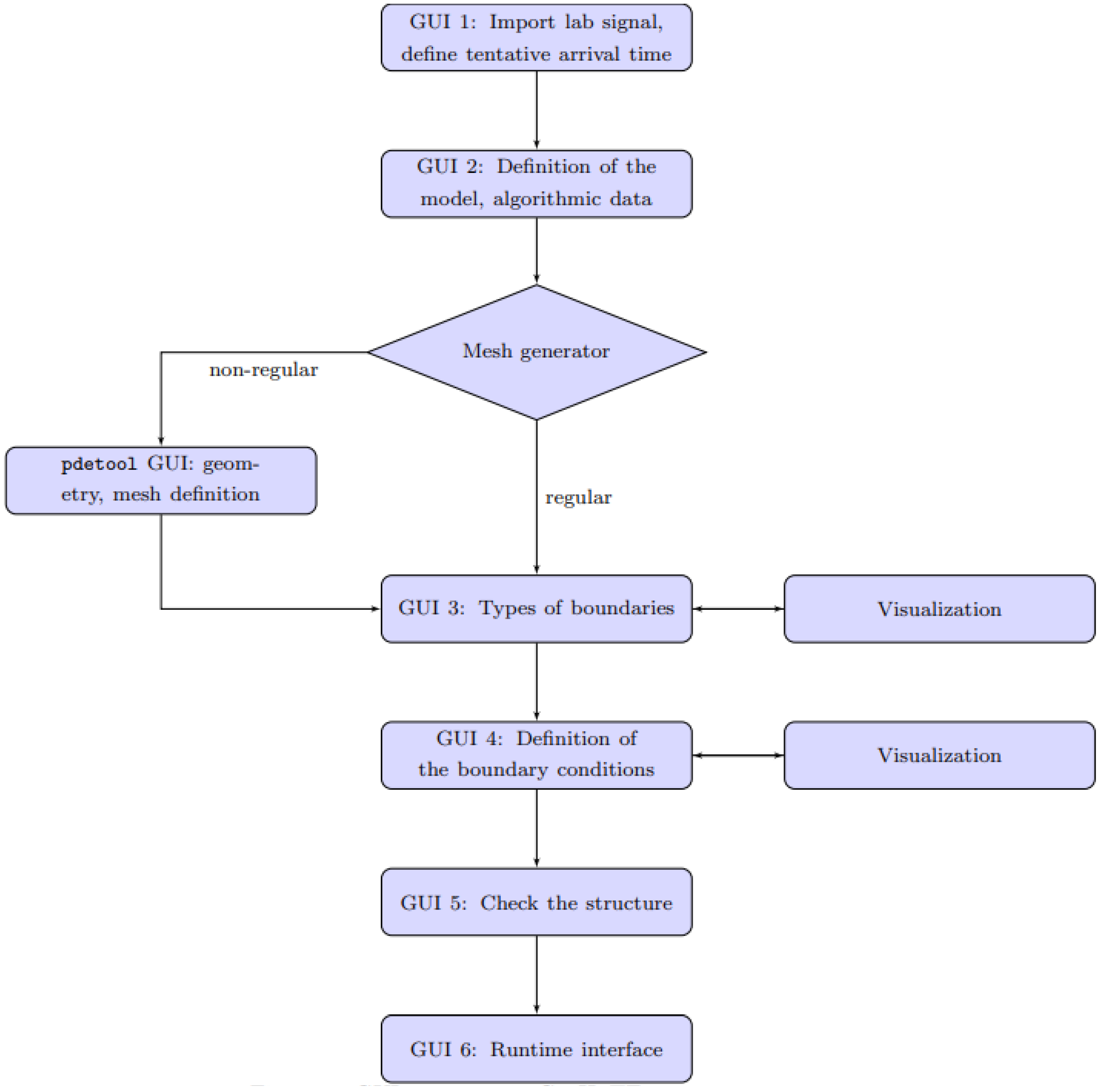
Data input and execution in GeoHyTE are controlled from six sequential GUIs, with free forward and backward navigation, complemented by the Matlab-native pdetool interface for the generation of non-regular meshes and a detailed visualisation interface.

An overview of the GUI structure is presented in Figure 2. GUI 1 handles the visualisation and interpretation of the experimental input signal, including the definition of the tentative arrival time and correlation window. The finite element model of the bender element experiment is defined through GUIs 2 to 5. GUI 6 is the runtime interface. It remains open during the execution of GeoHyTE and hosts the cross-correlation plots and the current estimates for the arrival time of the shear wave as well as for the shear modulus.

The next sections illustrate the data input, execution, and output of GeoHyTE using one of the International Parallel Test benchmarks as an example.

3.2.2. Experimental Data

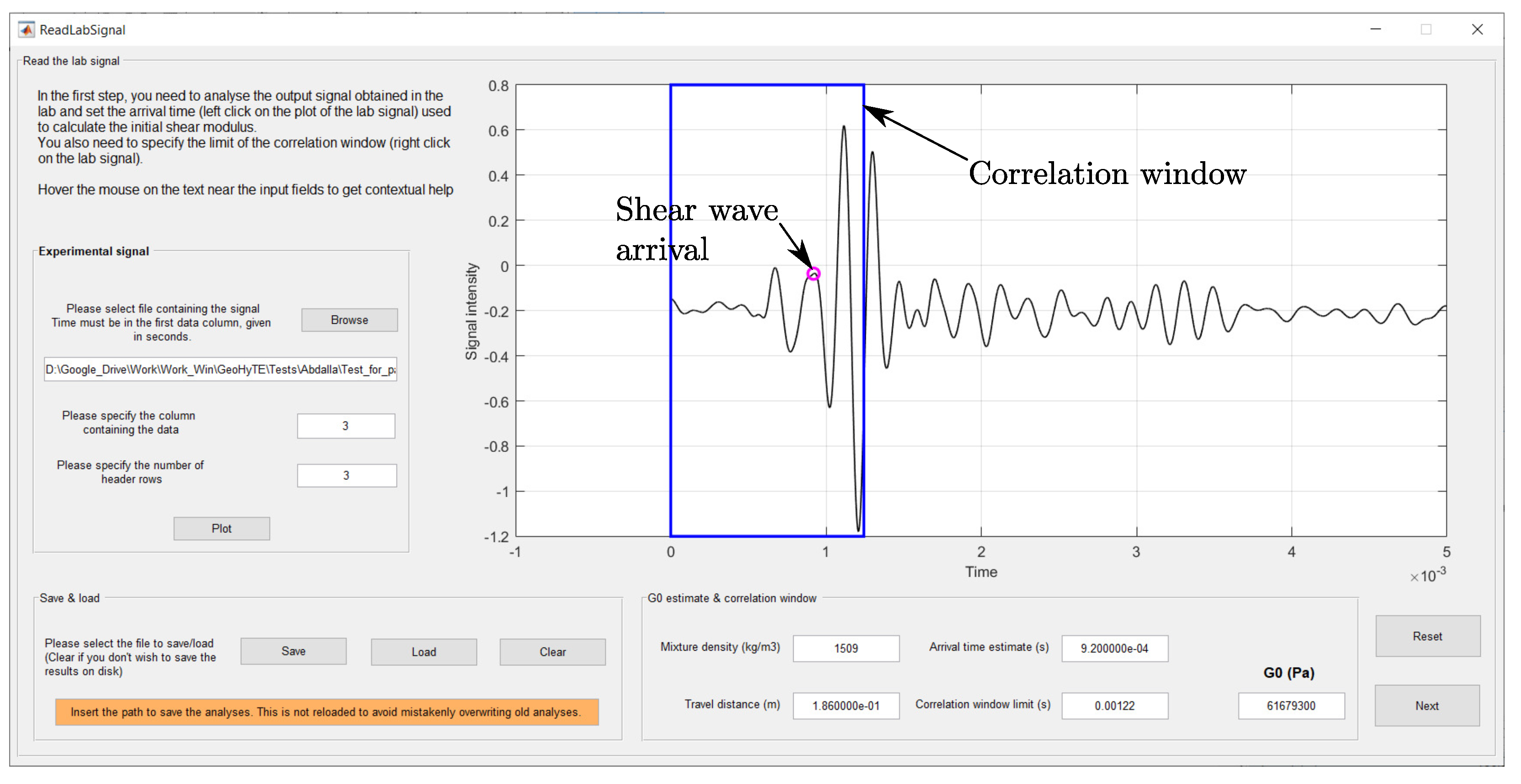
GeoHyTE’s first GUI is illustrated in Figure 3. It accommodates the information coming from the experiment, including the output signal, the mixture density of the material, and the travelling distance of the shear wave. This information, together with the tentative arrival time, is needed to compute the initial shear modulus.

The experimental data are loaded and plotted from the Experimental signal panel. The input file should contain the data in tab-separated columns, where the first column should be the time, measured in seconds. The file may contain as many columns and as many header lines as desired. The column containing the output signal that should be loaded and the number of header lines should be specified in the same panel. After the $\boxed{\mathrm{Plot}}$ button is pressed, the plot of the output signal appears.

As shown in Section 3.1.3, the user needs to define the correlation window and the tentative arrival time. Left click on a point on the plot sets that point as the arrival time of the shear wave and marks it with a magenta circle. Right click on a point on the plot sets that point as the limit of the correlation window, which is marked in blue on the plot. Edit boxes Arrival time estimate and Correlation window limit are filled automatically with the instants selected by the user. However, these values can be edited by the user, if needed. The first shear modulus estimate is also filled automatically in the $G0$ edit box.

3.2.3. Definition of the Finite Element Model

The definition of the finite element model of the bender element test involves three steps: algorithmic and material parameters; finite element mesh; and boundary conditions.

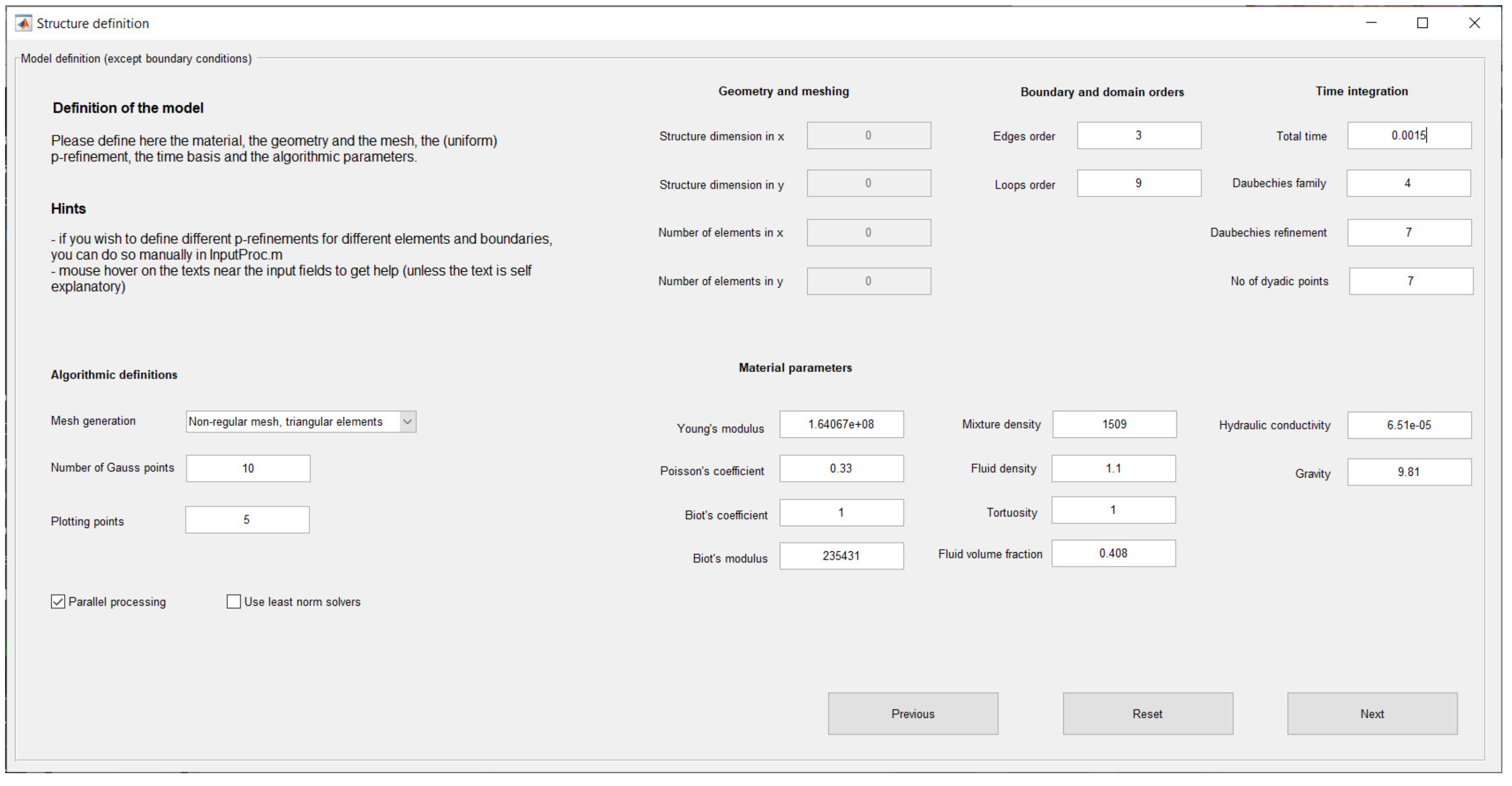
GUI 2: Algorithmic and Material Parameters

The layout of GUI 2 is presented in Figure 4. The algorithmic parameters include the refinements of the time and space bases, the type of mesh generator to be used, and some options that control the execution of the finite element analysis.

The definition of the Daubechies wavelet bases for the approximation of the time variation of the unknown fields requires the specification of the family number, the order of refinement, and the number of dyadic time points for the computation of the solution. The number of dyadic points $\left(d\right)$ controls the resolution of the time–history solutions, which are plotted in $2^d+1$ equally spaced time points between zero and the total time of the analysis, which is also specified in the Time integration zone of GUI 1.

As shown in Section 3.1.2, hybrid-Trefftz elements use dual approximation bases in the domain and on the essential (kinematic, elastic, absorbing) boundaries. The domain approximation, constrained to satisfy all domain equations but none of the boundary conditions, consists of Bessel functions in the radial direction and exponential functions in the tangential direction, expressed in a local referential centred in the barycentre of each finite element. Order $n_D$ of the domain basis should be input in the Loops order field. The boundary bases are used to enforce the boundary conditions on the functions contained in the domain bases. They are built on complete Chebyshev polynomials, expressed in a boundary local referential. Order $n_{\mathrm{\Gamma }}$ of the boundary bases is input in the Edge order field. Hybrid-Trefftz elements support distinct definitions of the orders of domain and boundary bases in different elements and essential boundaries, respectively. However, for simplicity, the GeoHyTE default is to use the same orders in all elements and essential boundaries. Advanced users can easily define distinct orders programmatically. To observe the kinematic indeterminacy condition, the total number of functions contained in all domain bases must be larger than the total number of functions contained in the boundary bases. While the compliance with this condition in the limit may be cumbersome to secure, its loose compliance is always ensured by using domain and boundary orders such that

$$\begin{array}{c}\hfill n_D\ge 2\left(n_{\mathrm{\Gamma }}+1\right)\end{array}$$

(6)

The geomechanical properties of the material consistent with Biot’s theory [29] must be specified in the Material properties zone. The definition of some of these properties may be challenging for analysts less acquainted with Biot’s theory. To support GeoHyTE’s users in such situations, a short description of the involved parameters and the expressions used to compute them are given in Appendix A.

The algorithmic parameters that need to be defined in GUI 2 are the number of Gauss quadrature points, the number of plotting points, the options to solve the spectral problems in parallel and to use iterative solvers for the algebraic system, and the type of the mesh generator. The Gauss quadrature points are used for the (boundary) integrations required to construct the finite element system. Insufficient Gauss points may lead to large errors in the coefficients, while an excessive number of points increase the computational time. The number of plotting points controls the resolution of the solution representation in each finite element. The total number of points where the solution is plotted inside each element is equal to the number of plotting points squared.

The Parallel processing option triggers the distribution of the time-discretised problems to be solved by all cores of the machine. The option requires the Parallel Processing Toolbox, but drastically increases the efficiency of the execution. Matlab’s advanced users can control the number of cores that perform the calculations programmatically.

The Use least norm solvers option enables GeoHyTE to use least norm solvers on ill-conditioned solving systems. However, the convergence to a strong solution using such solvers can be extremely slow. If the solving system is ill-conditioned, decreasing the order of domain and boundary refinements and increasing the mesh refinement is typically the safest option.

Geometry and Meshing

GeoHyTE offers regular and non-regular mesh generators.

The regular mesh generator divides rectangular domains into rectangular finite elements of similar sizes. It can only be used for rectangular, simply connected geometries. The definition of the geometry is produced in the GUI 2 (Geometry and meshing zone) by specifying the structural dimensions and the number of finite elements in each Cartesian direction. The origin of the global referential is taken by default in the lower left corner of the domain and cannot be changed.

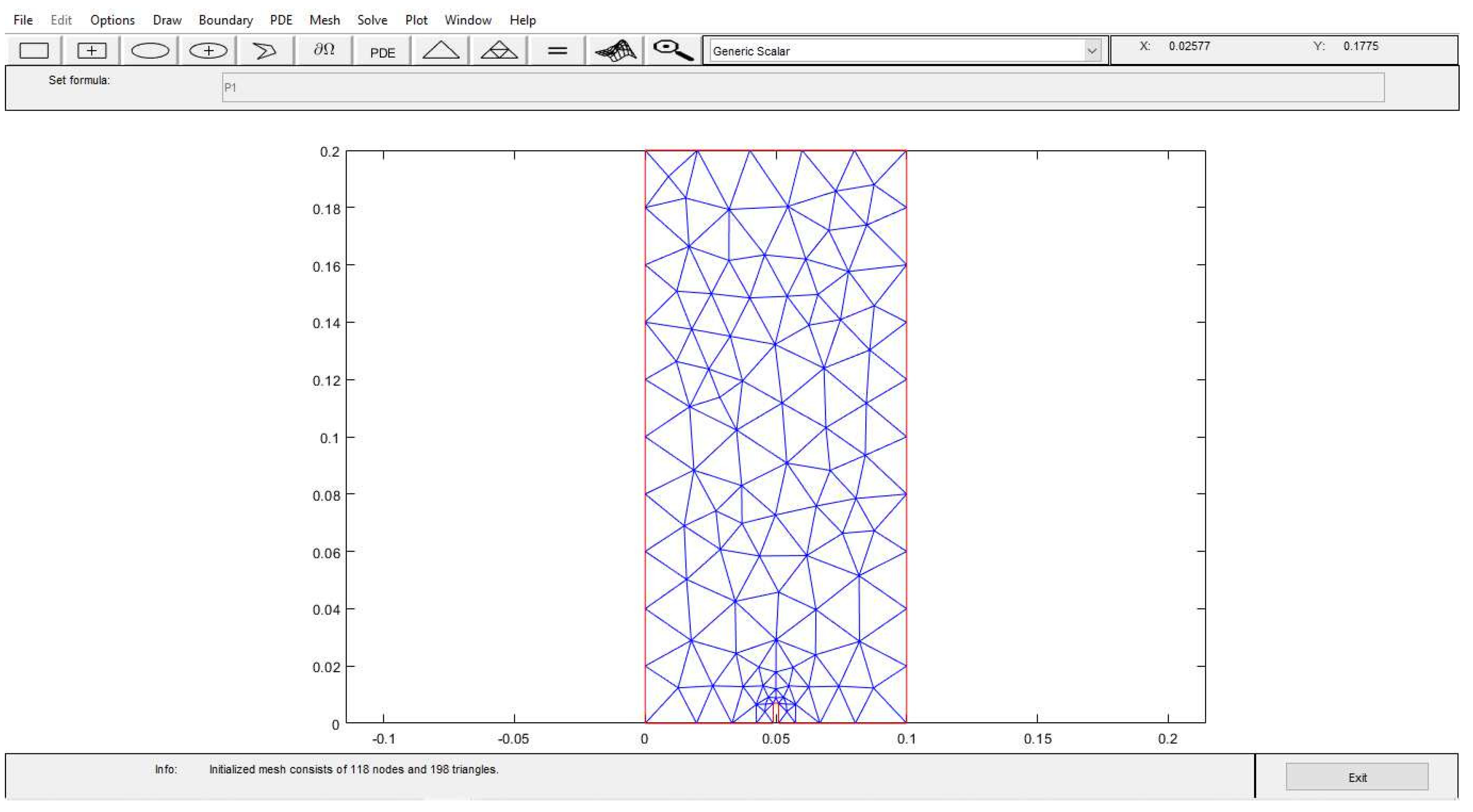
The non-regular mesh generator is based on the Matlab–native pdetool interface. It features a simple click-and-drag interface for the geometry creation. Basic shapes such as rectangles, ellipses, and polygons are used as building blocks and all geometries are combinations of such shapes. The non-regular mesh generator can be used for any type of geometry, simply or multiply connected, which is meshed into triangular elements (see Figure 5).

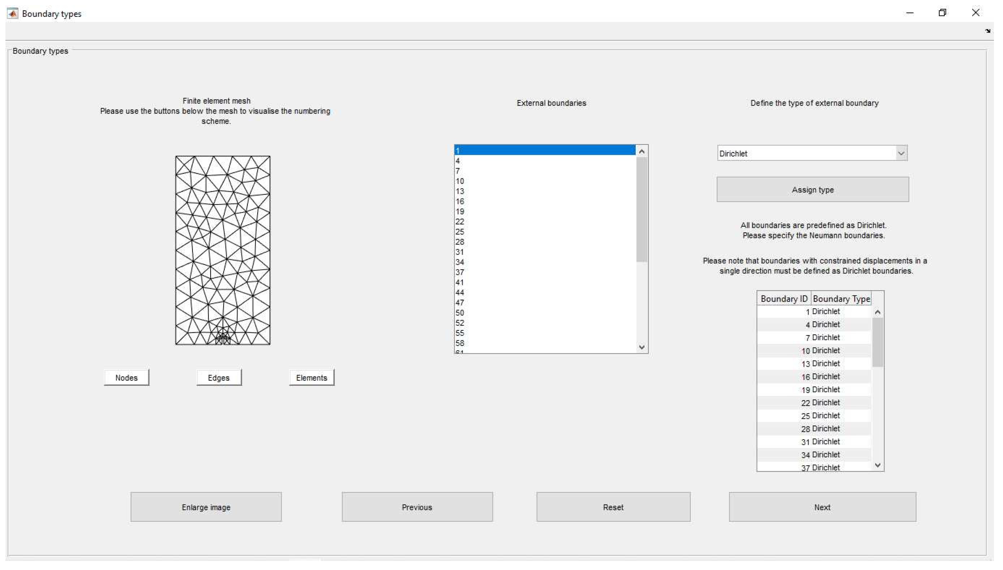
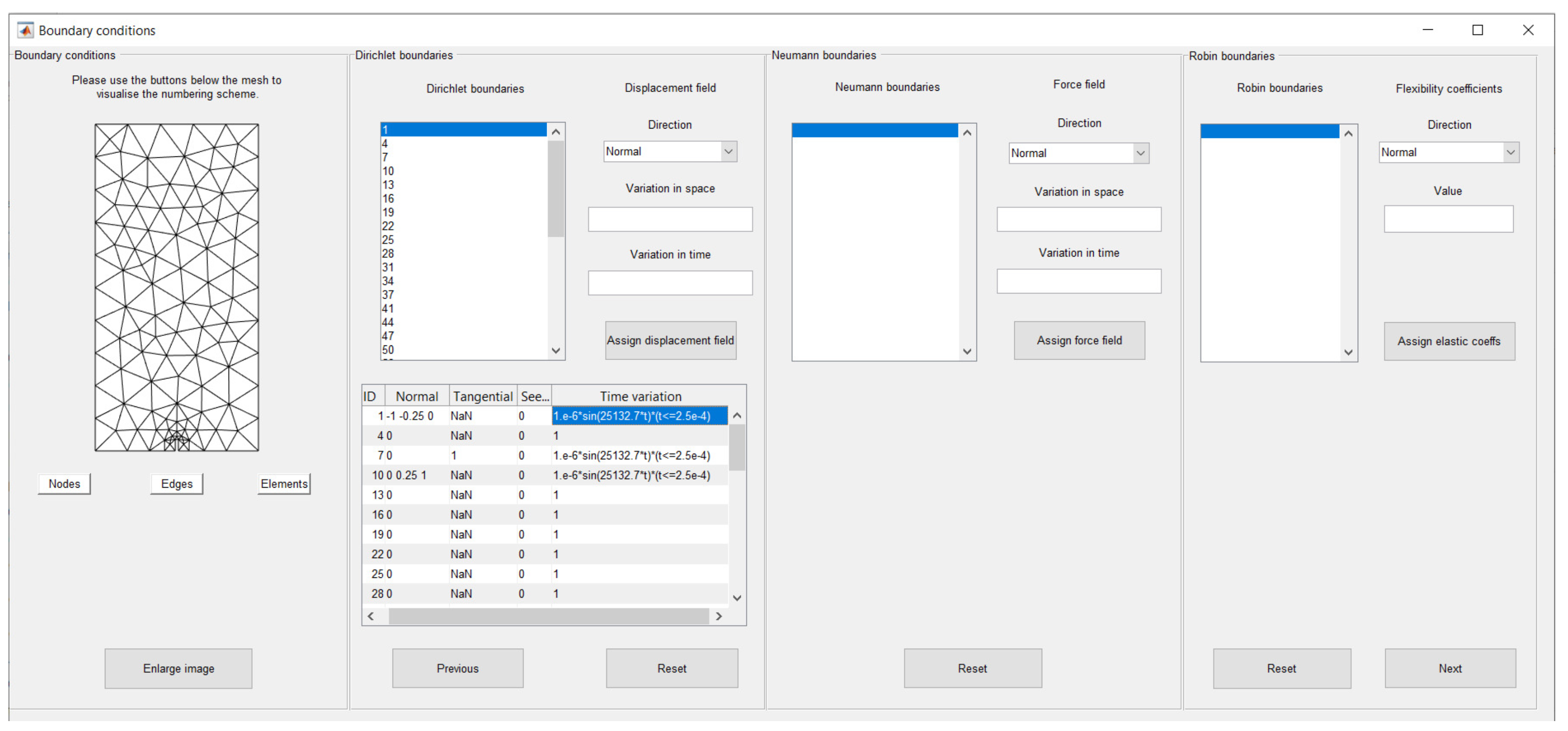
Boundary Conditions

The boundary types are defined in GUI 3 (see Figure 6). All exterior boundaries are listed in the External boundaries table. Four types of boundaries may be assigned. Displacements in the solid phase and the fluid seepage are enforced on the Dirichlet (kinematic) boundaries. On Neumann (static) boundaries, the applied forces and pore pressures are specified. Robin boundaries are elastic boundaries, where flexibility coefficients must be defined to enforce a linear relationship between displacements and stresses. It is noted that Robin boundaries are considered impervious, meaning that the fluid seepage in their normal direction is assumed null. Robin boundary conditions can be used to control the impedance difference between the geomaterial and the testing apparatus to control the wave energy reflected back into the material from the sample apparatus interface. Finally, absorbing boundaries are designed to absorb incoming waves. They are useful to set the impedance difference between the sample and the testing apparatus to nearly zero, thus preventing wave reflections.

On the left of GUI 3, a small scale image of the mesh created in the previous step is shown, along with three buttons that control the visualisation. If, as is the case of the mesh displayed in Figure 6, the image is too small for a clear visualisation of the structural data, a separate visualisation interface with zoom, pan, and data cursor capabilities can be accessed using the $\boxed{\mathrm{Enlarge}\mathrm{image}}$ button.

The values of the enforced boundary conditions are defined in GUI 4 (Figure 7) according to the boundary types defined in GUI 3. Information on the boundary conditions are required for Dirichlet, Neumann and Robin boundaries. The stiffness of the absorbing boundaries is computed automatically, based on the mechanical parameters of the material.

Dirichlet boundary conditions are defined by specifying the normal and tangential displacements in the solid phase and the normal fluid seepage. Neumann boundary conditions are defined by specifying the normal and tangential components of the applied forces in the solid phase and the pore fluid pressure. Boundary fields may vary in time and in space. They are therefore defined as the product of a function of time $\left(t\right)$ and a function of the side coordinate $\left(s\right)$:

$$\begin{array}{cc}& u_{{\mathrm{\Gamma }}_{n\left(t\right)}}(t,s)=u^t\left(t\right)\times u_{{\mathrm{\Gamma }}_{n\left(t\right)}}^s\left(s\right),\mathrm{on}{\mathrm{\Gamma }}_u\end{array}$$

(7)

$$\begin{array}{cc}& w_{\mathrm{\Gamma }}(t,s)=u^t\left(t\right)\times w_{\mathrm{\Gamma }}^s\left(s\right),\mathrm{on}{\mathrm{\Gamma }}_u\end{array}$$

(8)

$$\begin{array}{cc}& t_{{\mathrm{\Gamma }}_{n\left(t\right)}}(t,s)=t^t\left(t\right)\times t_{{\mathrm{\Gamma }}_{n\left(t\right)}}^s\left(s\right),\mathrm{on}{\mathrm{\Gamma }}_{\sigma }\end{array}$$

(9)

$$\begin{array}{cc}& {\pi }_{\mathrm{\Gamma }}(t,s)=t^t\left(t\right)\times {\pi }_{\mathrm{\Gamma }}^s\left(s\right),\mathrm{on}{\mathrm{\Gamma }}_{\sigma }\end{array}$$

(10)

The time variations of the boundary fields are specified as analytic expressions of time using any mathematical expression that can be interpreted by Matlab. Branched and discontinuous time variations can be input using logical operations. Conversely, the spatial component of the boundary conditions is defined by polynomials. The analytic expression of a polynomial of degree D is generated automatically by GeoHyTE based on the values of the field in $D+1$ equally spaced points along the boundary. Roller (sliding) supports, where the material can move freely in the tangential direction, can be defined by simply defining the tangential enforced displacements as NaN.

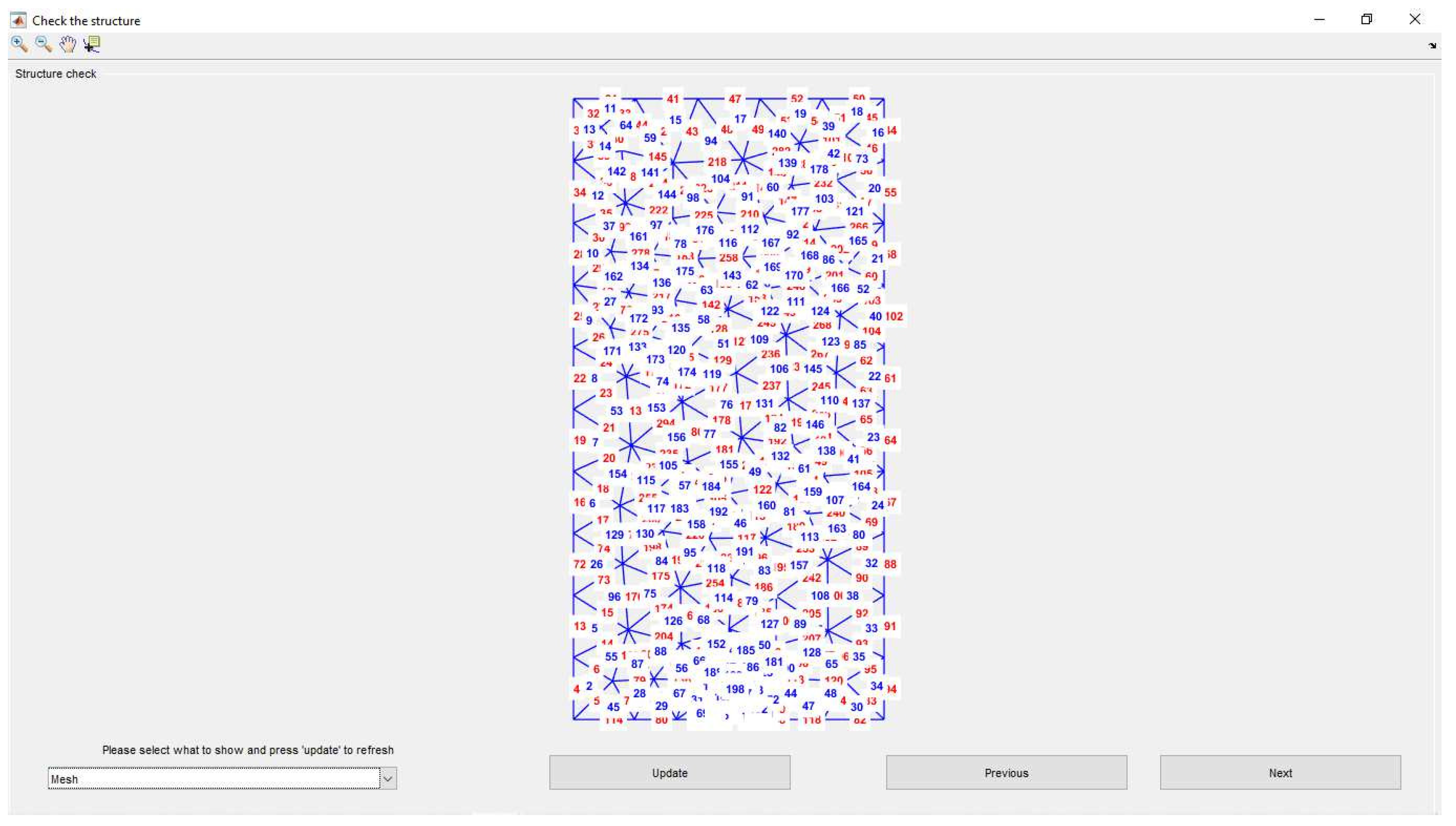
Verification

Before proceeding to the runtime interface, GUI 5 (Figure 8) allows the user to verify the input. GUI 5 is a simple interface, with a single pop-up menu to choose the desired information (mesh numbering or boundary conditions). Pan and zoom can be used to check the details of the structure.

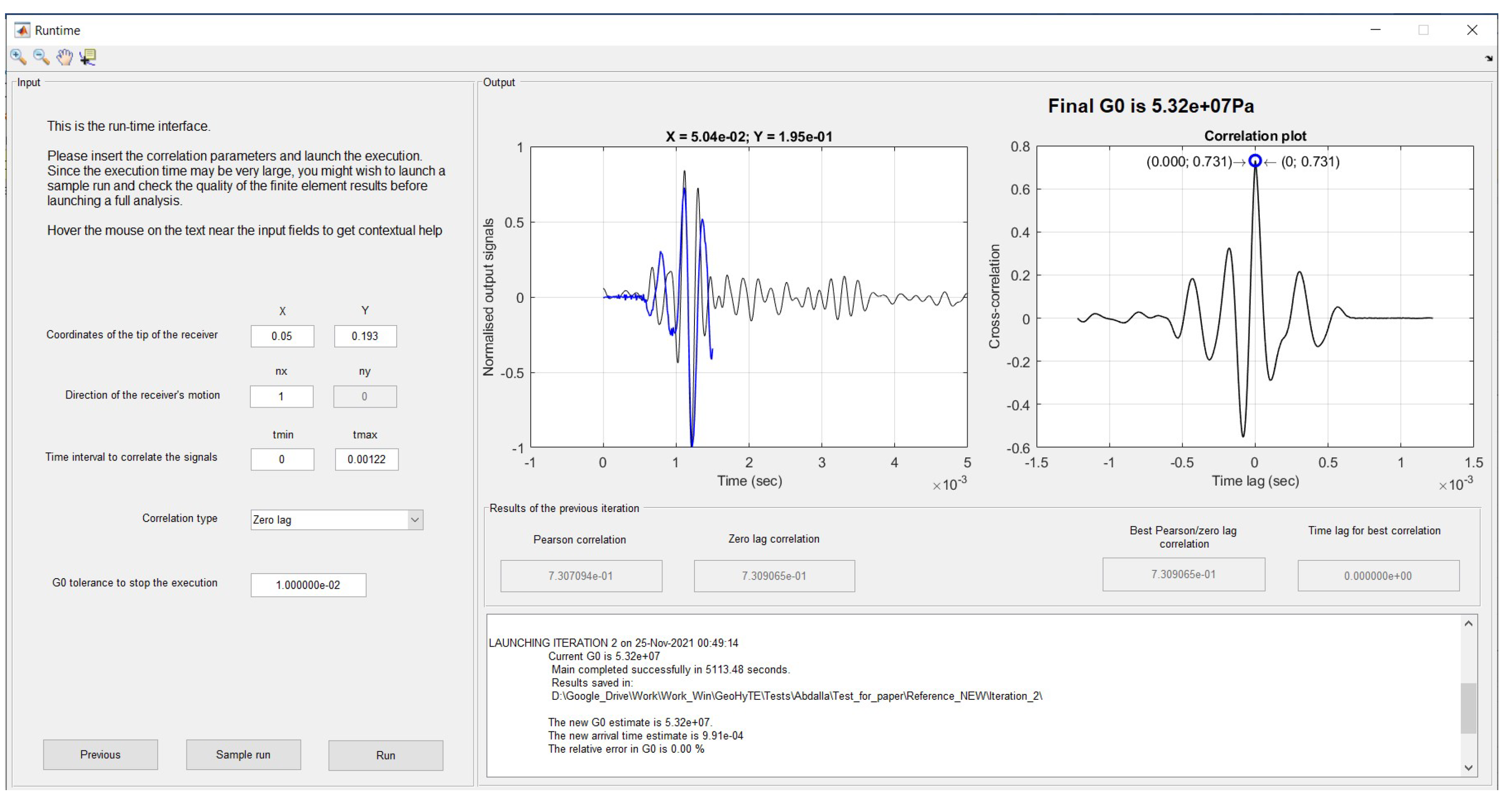
3.2.4. Runtime and Post-Processing

The last GUI is the runtime interface, which remains open throughout the whole analysis. It contains two panels: an input panel, with data required before running the analysis, and the output panel, displaying information generated by the solver.

On the left of GUI 6 (see Figure 9), the user must define the coordinates of the tip of the receiver and the components of the direction of the receiver’s motion in the global Cartesian referential used to define the domain’s geometry. Other important inputs are the tolerance for considering that a fixed point was found for the shear modulus and the type of correlation to be performed, namely without (zero lag) or with signal normalisation (Pearson).

Both $\boxed{\mathrm{Sample}\mathrm{run}}$ and $\boxed{\mathrm{Run}}$ buttons, situated in the lower part of the input panel, start the execution of the analysis. The sample run allows the user to foresee the expectable quality of the finite element solution at the lowest computational cost possible. Instead of analysing all spectral problems, GeoHyTE only runs the spectral problem with the largest participation factor in the final solution and writes an output file containing the (real parts of the) displacements in the solid phase, fluid seepage, total stresses, and pore pressures in the plotting points defined in GUI 2. The output file can be read using post-processing (visualisation) software like Paraview or Tecplot. If the quality of the sample is satisfactory, a full analysis can be launched. Otherwise, the user may wish to return to the definition of the model and improve the basis and/or the mesh refinement.

The right panel in GUI 6 is the output panel. On its upper part, two plots are shown after each iteration. The plot on the left shows the numerical (blue) and experimental (black) output signals, overlapped over the correlation window. The cross-correlation plot between the two signals is shown in the plot on the right. The instantaneous and best correlations are identified with blue and red circles, respectively. The bottom part of the right panel contains a log listing information regarding the current and previous iterations. When the analysis converges, the log also registers the final shear modulus estimate.

The displacement/seepage and stress/pore pressure fields in each (dyadic) time point are saved after each iteration in text files that can be read by external visualisation software.

4. Validation Using the International Parallel Test Benchmarks

The capability of GeoHyTE to converge to correct shear modulus estimates is studied in this section. The main objective of this validation campaign is to coin GeoHyTE as a mainstream interpretation method, along with the time and frequency domain methods.

A particularly problematic testing configuration reported in the International Parallel Test [12], namely the dry $K_0$-consolidated Toyoura sand with a vertical applied pressure of 50 kPa is taken as a reference. For this configuration, the International Parallel Test reports 45 measurements involving void ratios between $e=0.680$ and $e=0.800$ (typically $e=0.690$ and $e=0.770$, also used in this study), with $G_0$ readings ranging from $3.40$ MPa to 108 MPa, with an average value of the shear modulus of $44.10$ MPa. For each void ratio, the experiments are repeated eight times in full, i.e., the sample is removed from the envelope, dried and set up again. This strategy secures enough data to compare the shear moduli obtained using various time and frequency domain interpretation methods with those predicted by GeoHyTE and check the latter for consistency. A statistical analysis of these data is also performed.

4.1. Experimental Campaign

4.1.1. Bender Element System

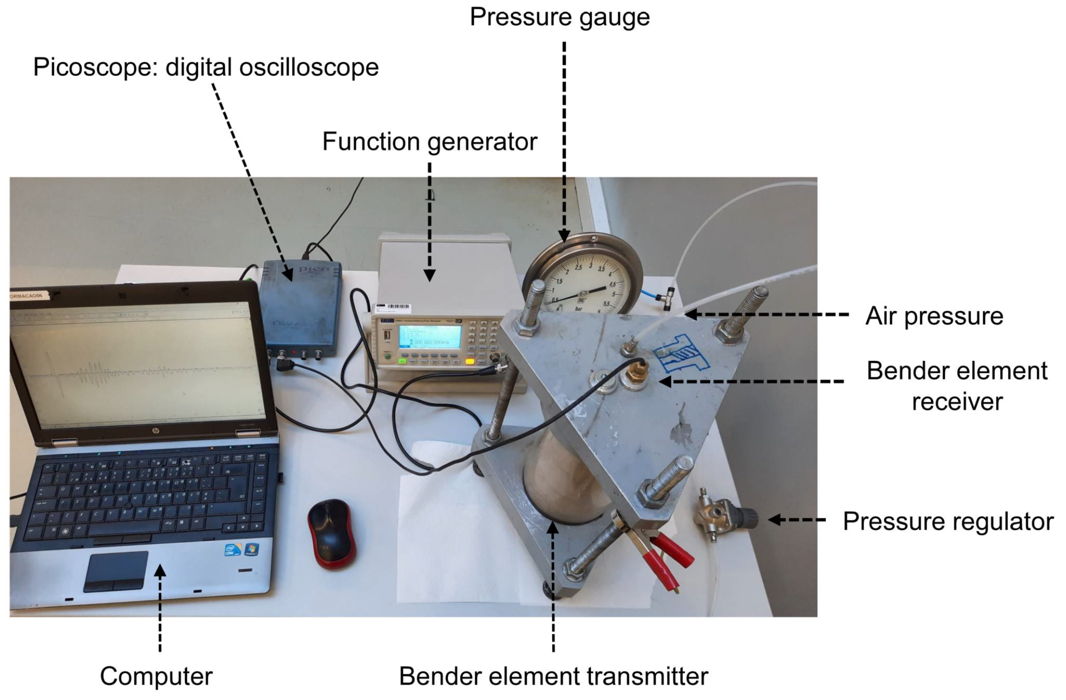
The bender element apparatus involves two T-shape transmitter and receiver bender elements embedded in standard inserts. The bender elements are supported by a function generator (Huntingdon TG2511) and a digital oscilloscope with two channels with sampling rates of 80 Ms/s and two of 20 Ms/s used to store and display the signals. A spectrum analyser software averages several measurements to filter the noise out from the output signal. Figure 10 presents an overview of the experimental apparatus.

4.1.2. Material and Testing Procedure

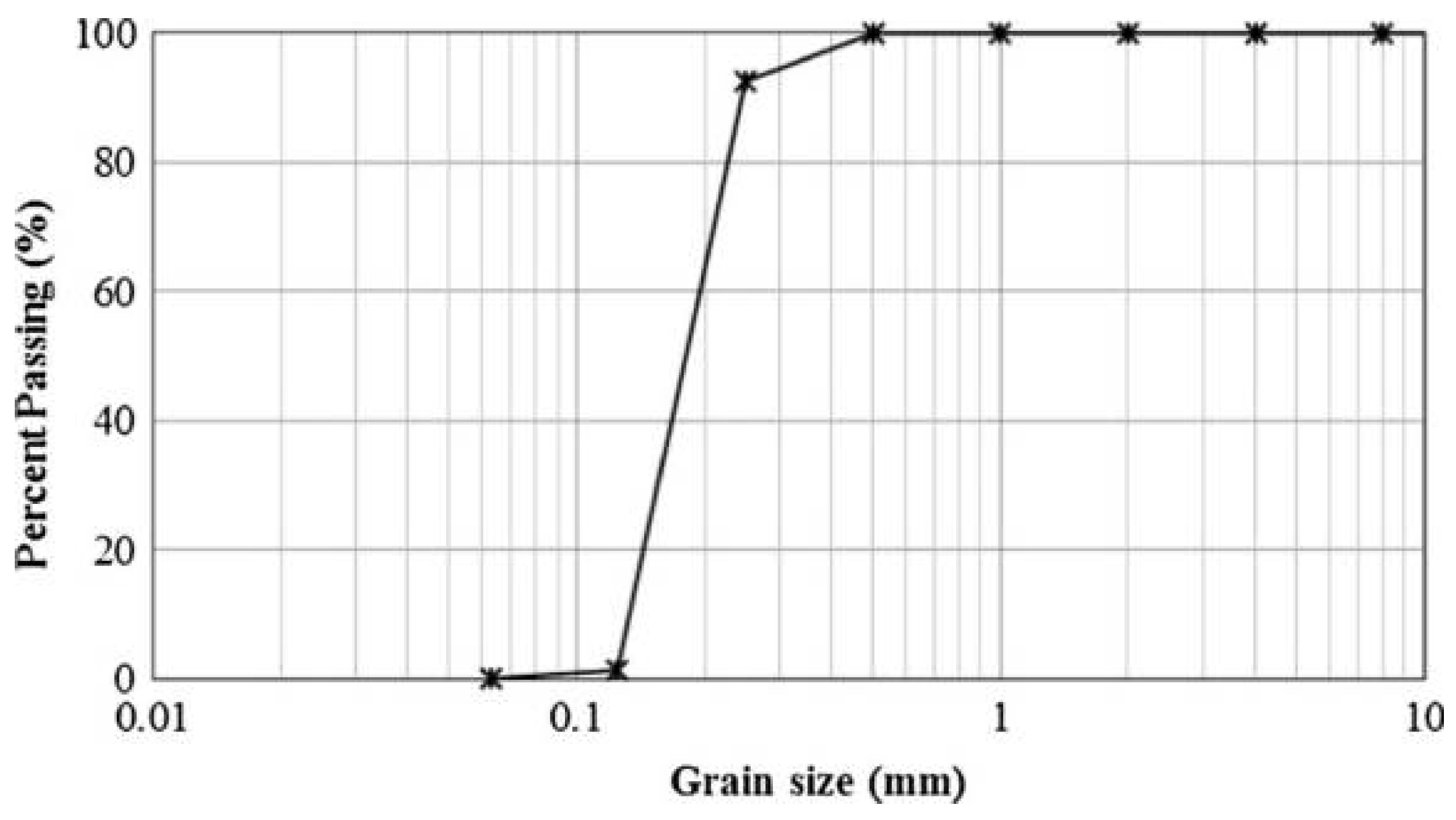
Toyoura sand is a benchmark geomaterial used in the International Parallel Test [12]. It consists of quartz, limestone, and mica, among other materials. The test described here is performed on dry samples of uniformly graded material, with round-shaped particles larger than 75 µm in diameter. The physical properties of the Toyoura sand are shown in

Table 1. Physical properties of Toyoura sand [19].

Property	Value
Specific gravity	2.65
Maximum void ratio	0.968
Minimum void ratio	0.628
Maximum dry density $\left(\frac{\mathrm{g}}{{\mathrm{cm}}^3}\right)$	1.628
Minimum dry density $\left(\frac{\mathrm{g}}{{\mathrm{cm}}^3}\right)$	1.347
Mean grain size, $D_{50}$ (mm)	0.15
Coefficient of uniformity	1.43

, and its grain size distribution is presented in Figure 11.

The Toyoura sand specimens are prepared according to the dry tamping method. The material is left to dry in an oven for 24 h to remove any trace of initial moisture. Then, five layers of geomaterial, dosed to achieve the desired void ratio, are gradually poured into the mould with constant drop height. Each soil layer is levelled and compacted to the desired height with a tamper.

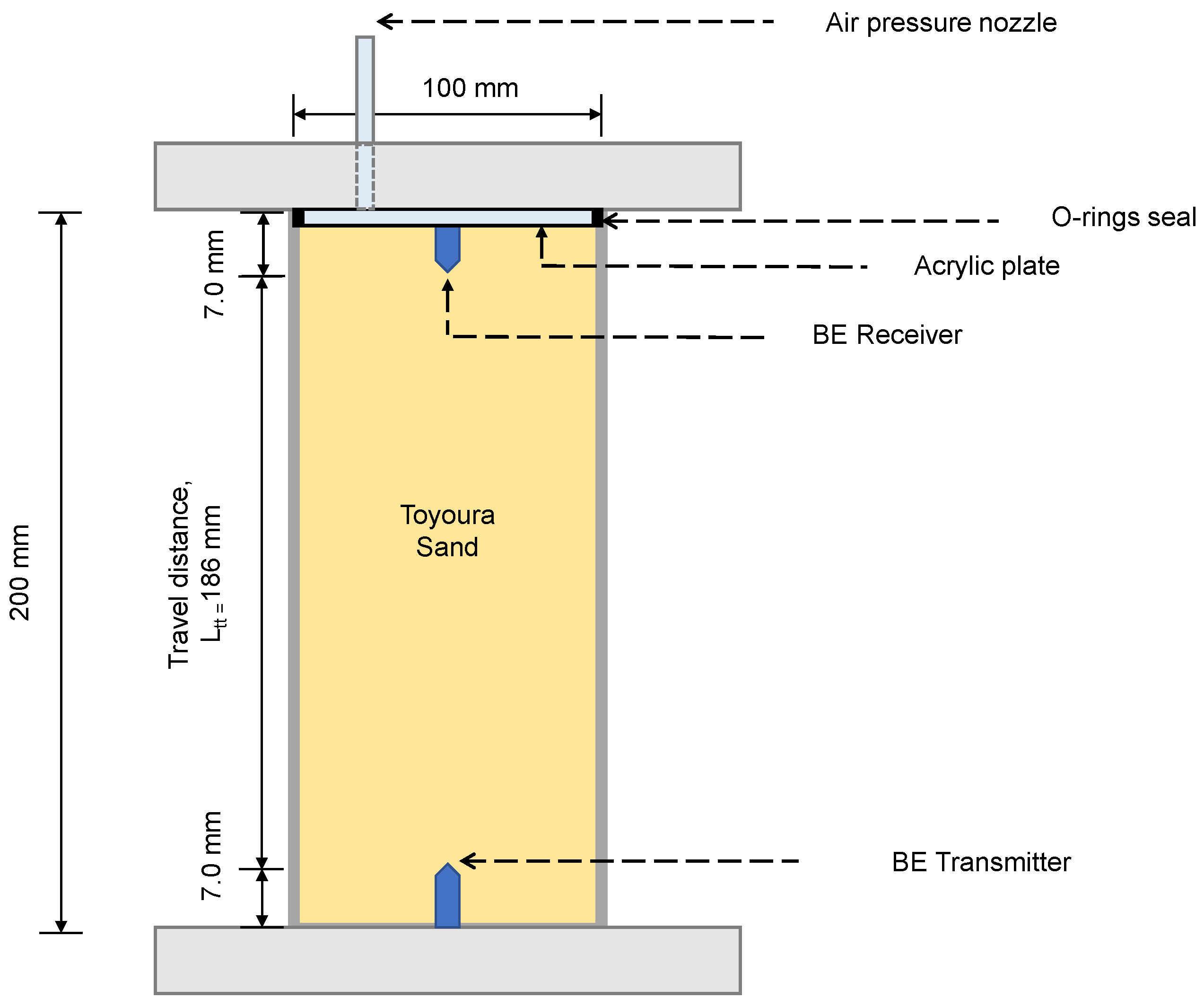
The bender elements are installed in a container filled with Toyoura sand. It consists of a cylindrical acrylic mould, a base platen, and a top platen (see Figure 12). The mould is 200 mm in height and has an internal diameter of 100 mm. The transmitter and receiver bender elements are embedded in the centres of the base and top platens. The top platen allows for the application of vertical pressure through a pressure nozzle, at the top of the specimen, under K0 conditions.

4.2. Shear Modulus Extraction

The techniques used for the interpretation of the 16 tests (8 for each void ratio) are illustrated on one of the output signals ($e=0.690$). The results of the other tests, analysed statistically in Section 4.3, are obtained in the same way.

4.2.1. Time Domain Interpretation Techniques

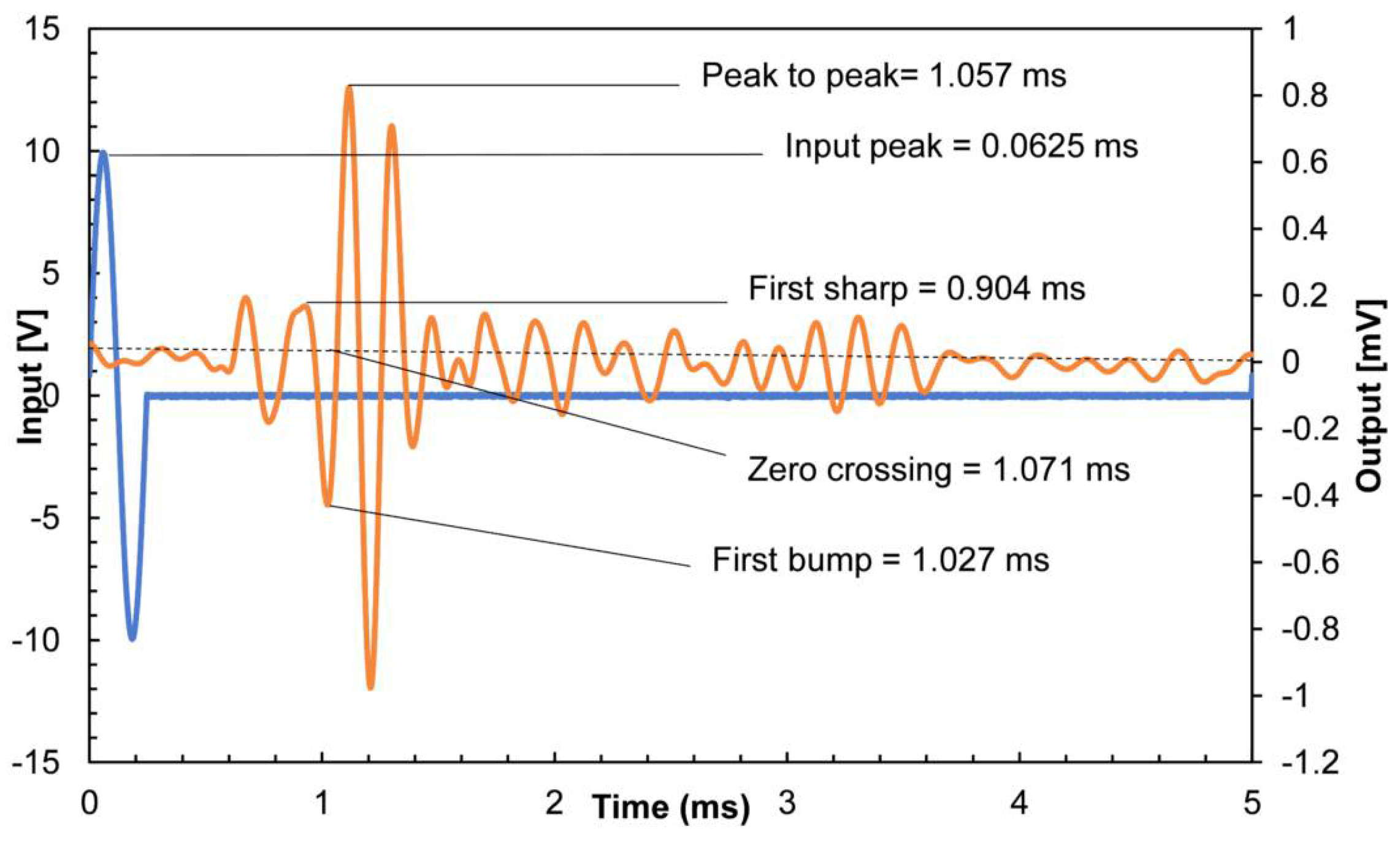
The input and output signals obtained in the bender element test are presented with blue and orange lines in Figure 13. The input signal is a single sine pulse with a frequency of 4 kHz. The output signal presents the interpretation challenges that typify bender element experiments. For instance, the first significant signal occurs around $0.65$ ms, but is disregarded here because the numerical models suggest it is caused by compression waves, not by shear waves. However, in the absence of this information, it could be used as an arrival indicator, leading to very erroneous results. The input and output signals use different intensity scales to enable the clear visualisation of the latter.

Three of the four classes of time domain interpretation techniques presented in Section 2.1 are used to obtain the arrival time from the plots presented in Figure 13. The method based on the second arrival is not employed as the second arrival signal is too weak.

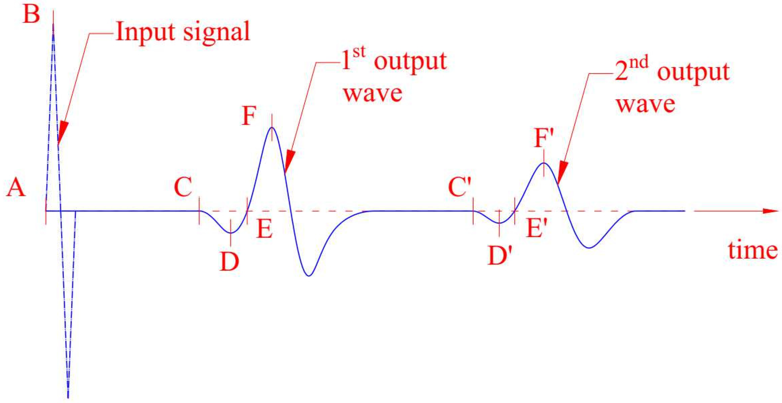
Interpretation Using Characteristic Points

The three characteristic points are defined in Section 2.1.1 and identified on the output signal in Figure 13. The first three lines of

Table 2. Shear moduli obtained with point picking methods.

Characteristic Point	Arrival Time (ms)	${\mathit{G}}_0$ (MPa)
First sharp	0.904	64.14
First bump	1.027	49.66
Zero crossing	1.071	45.66
Peak-to-peak	1.057	46.88

show the arrival times and the shear moduli corresponding to each of the characteristic points. The travel distance is defined between the tips of the transmitter and receiver, and the shear modulus is computed according to Expression (1).

Interpretation Using Peak-to-Peak Distance

The peak-to-peak distance is measured between the maximum amplitudes of the input and output signals, as seen in Figure 13. The travelling time obtained according to this technique and the corresponding shear modulus are listed in the fourth line of Table 2.

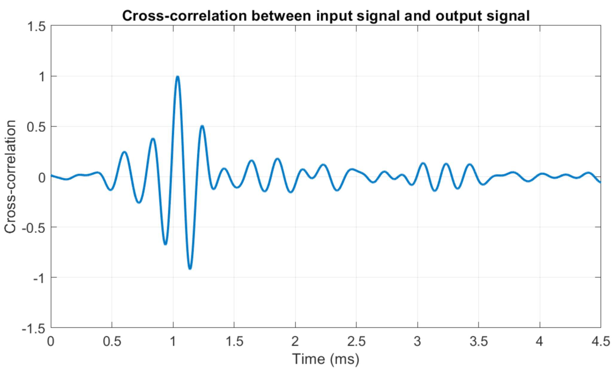
Cross-Correlation

The cross-correlation between input and output signals is computed according to Expression (4). The cross-correlation plot, shown in Figure 14, presents a clear peak at $1.037$ ms, which corresponds to a shear modulus of $48.71$ MPa.

4.2.2. Frequency Domain Interpretation Techniques

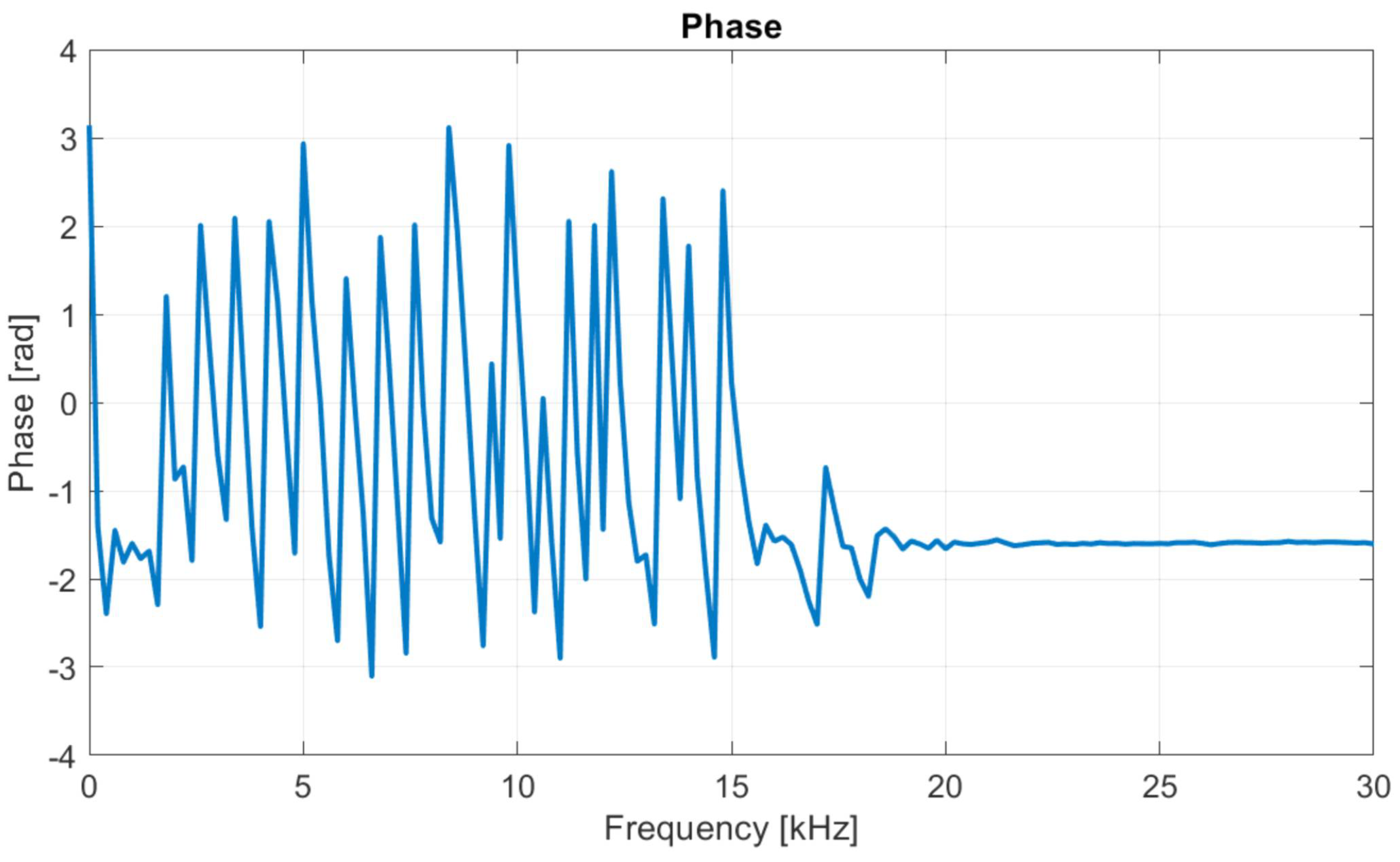
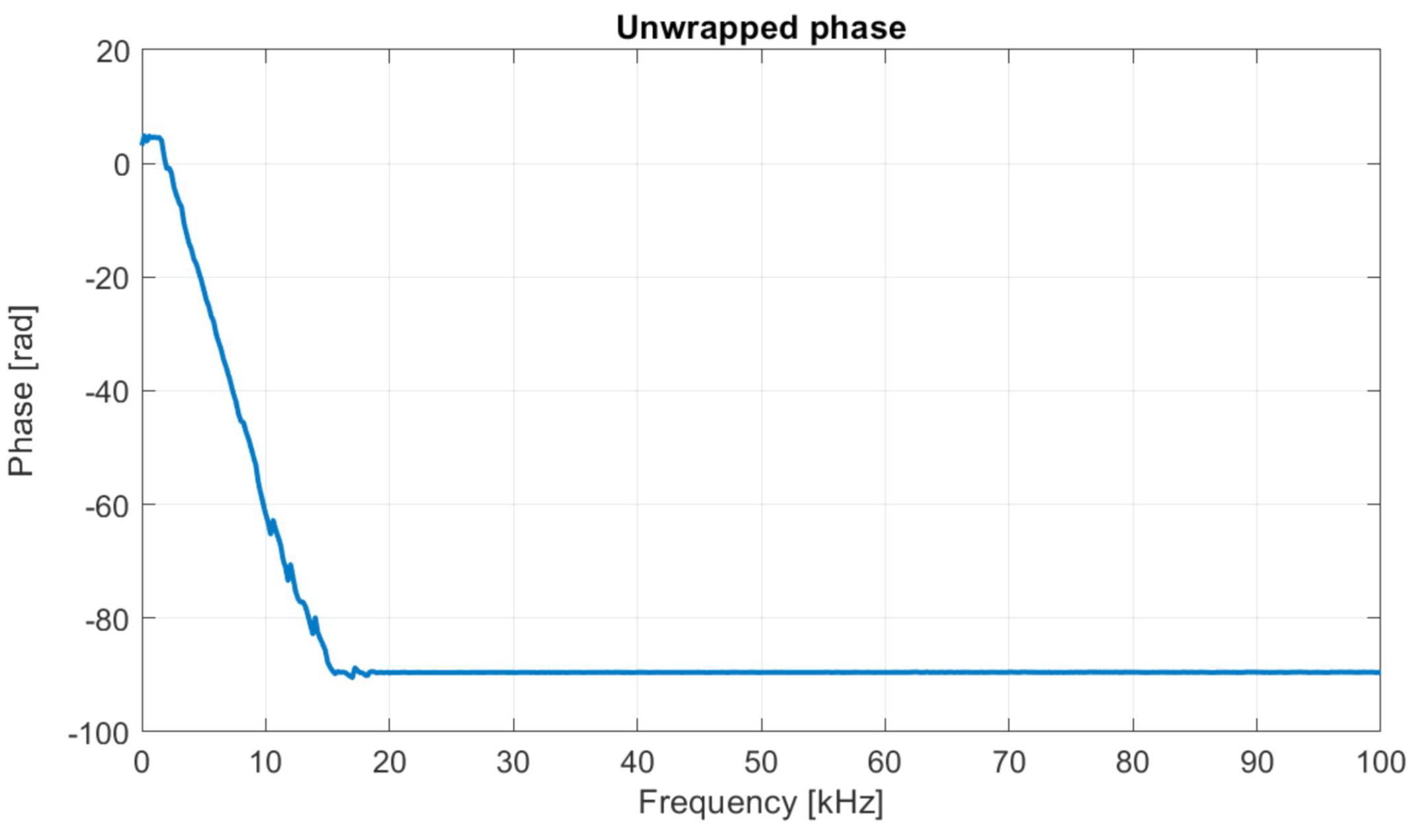
The cross-spectrum of input and output signals is obtained from the Fast Fourier Transform of both signals (Section 2.2). Figure 15 shows the phase relationship between input and output signal. The phase relationship is well defined in the region from 2 kHz to 15 kHz.

An unwrapping algorithm is used to convert the phase data into the unwrapped phase function, shown in Figure 16. The relationship is seen to be broadly linear. The arrival time of $1.220$ ms is determined from the average slope of the unwrapped phase relationship using Equation (2). This corresponds to a shear modulus estimate of $35.19$ MPa. As expected, the cross-spectrum techniques yield a lower shear modulus compared to time domain methods, caused by an estimated shear wave velocity that is 12 to 25% smaller than those obtained with the time domain methods.

4.2.3. Automatic Shear Modulus Extraction Using GeoHyTE

In GeoHyTE, the definition of the computational model follows the steps described in Section 3.2. The plots given there as GUI examples are obtained on this test case and are not reproduced here to avoid redundancy. The output signal, presented in Figure 13, is loaded into the first GUI (Figure 3), and the tentative arrival time, $t_{arr}=0.920$ ms, and correlation window of $1.220$ ms are selected. The arrival time corresponds to an initial estimate of the shear modulus of $G_0^1=61.68$ MPa. The correct choice of the tentative arrival time is not of great importance, as discussed at length in Section 5.1.

The finite element model is defined in the following user interfaces, as presented in Figure 4, Figure 5, Figure 6, Figure 7, Figure 8 and Figure 9. The subsequent run of the model converges in two steps, producing the output presented in Figure 17 and Figure 18.

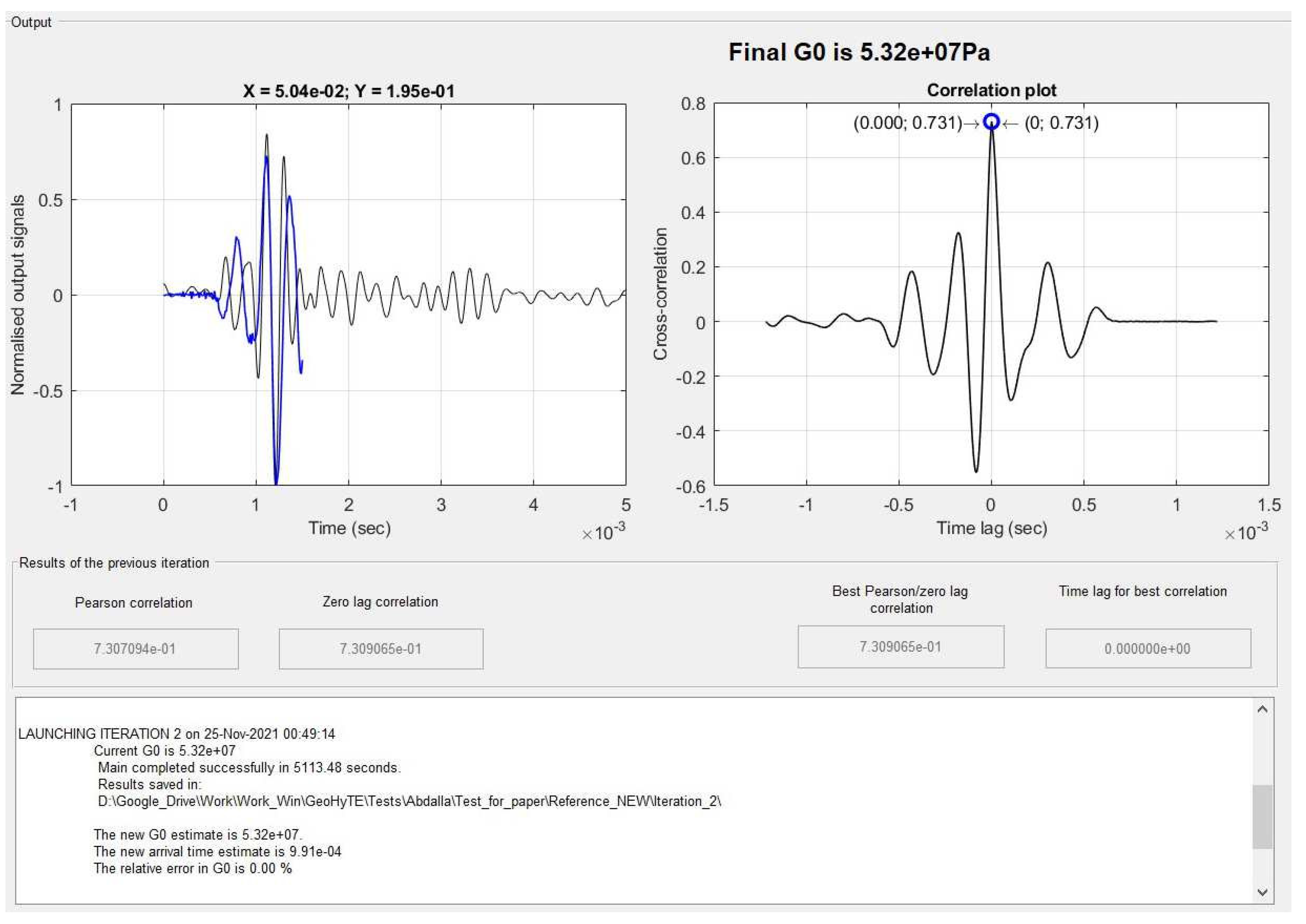
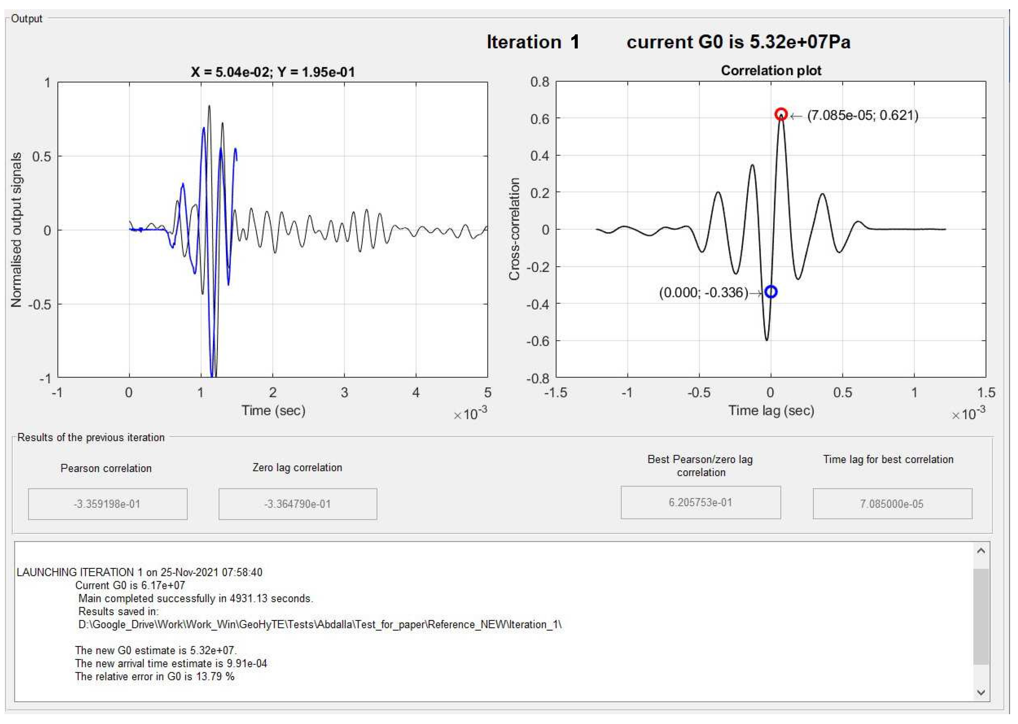
After the first run, the instantaneous correlation between the numerical and experimental output signals is scored at $-0.336$, as indicated by a blue circular marker in the plot on the right, which is a low correlation. However, the maximum correlation, found $7.085\times {10}^{-2}$ ms to the right, looks more promising, with an estimate value of $0.621$. The tentative arrival time is incremented with the time lag to the maximum correlation, that is, $t_{arr}=0.920+7.085\times {10}^{-2}=0.991$ ms, to which a new tentative shear modulus of $G_0^2=53.20$ MPa corresponds. This is the value used in the second iteration. These findings are automatically logged in the lower part of the output zone.

After the second run (Figure 18), the instantaneous correlation is also the maximum correlation, with a score of $0.731$, meaning that the fixed point of the shear modulus is found. Its final value is thus $G_0=53.20$ MPa, which is delivered to the user.

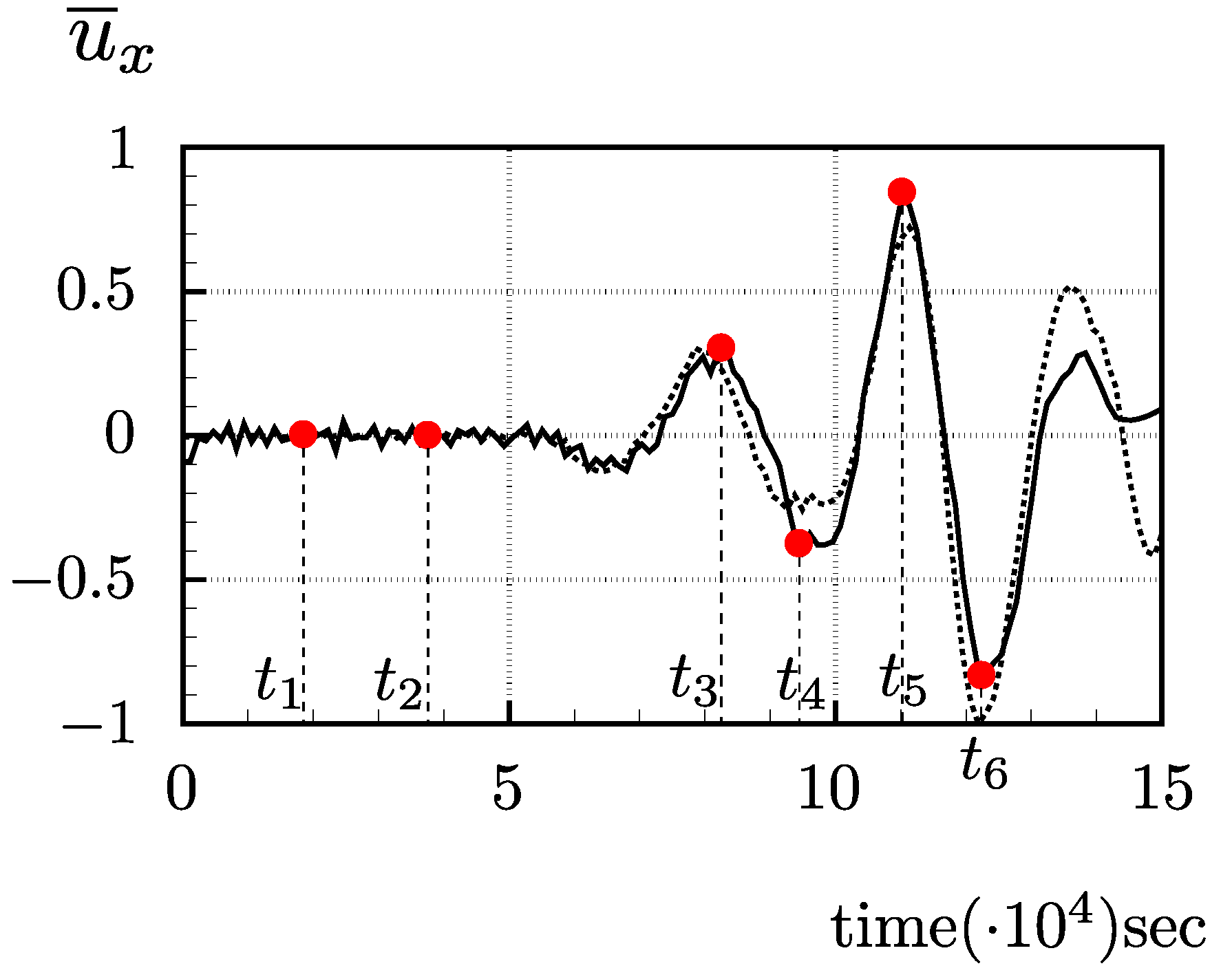
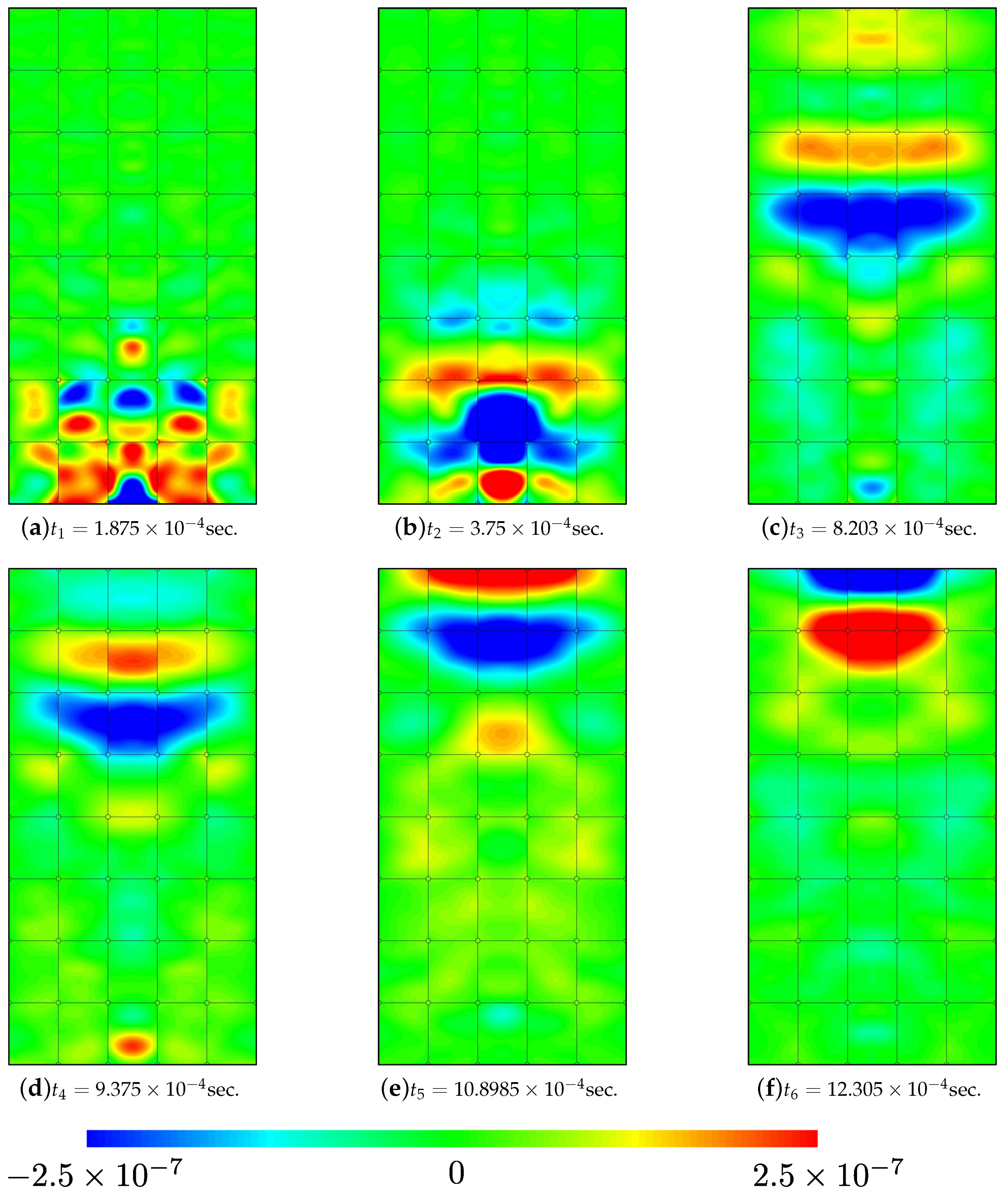
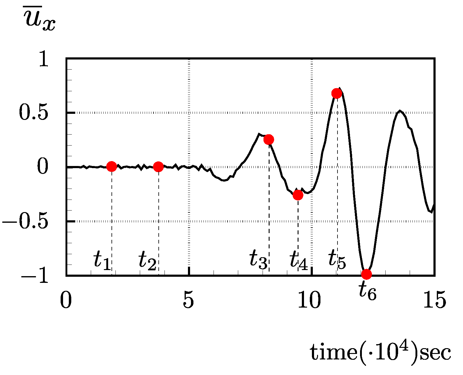
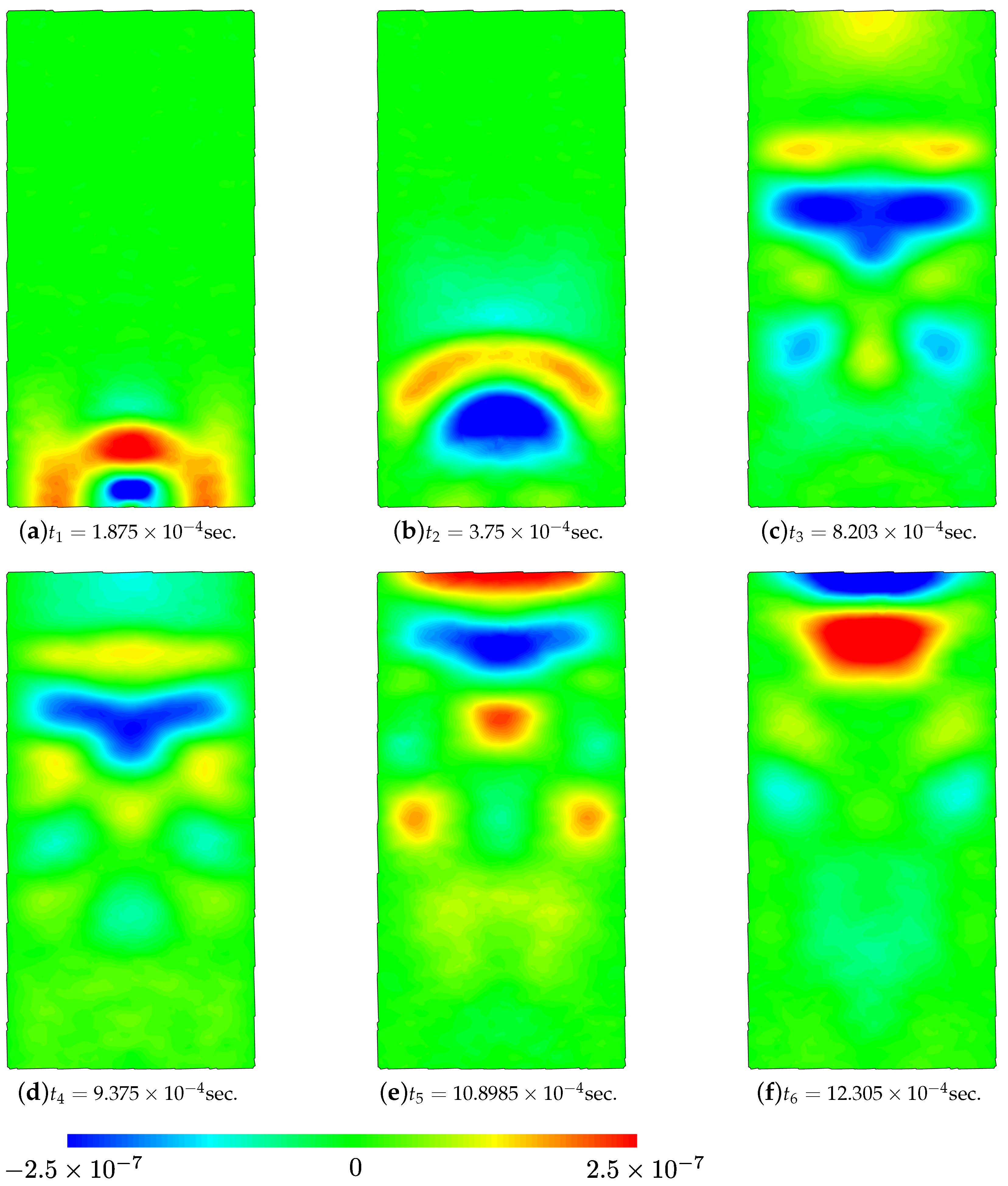
The time–history of the horizontal displacements at the tip of the receiver, normalised to their maximum amplitude, is presented in Figure 19. For a better illustration of the finite element solution, the horizontal displacement solutions over the whole domain are plotted in Figure 20 at key instants $t_1$ to $t_6$, indicated in Figure 19.

The first two instants correspond to the generation of the shear wave near the transmitter and to its early propagation after the motion of the transmitter ceases. The shear waves are clearly visible and their propagation from the transmitter to the receiver can be easily followed visually throughout the plots. The first significant oscillation in the numerical output occurs around points $t_3$ and $t_4$ and corresponds to the early arrival of compression waves reflected from the lateral envelope of the sample (Figure 20c,d). Although compression waves trigger lateral motion of smaller amplitude than shear waves, their criss-cross propagation through the sample can also be followed visually. Finally, the arrival of the shear wave and its reflection from the top platen are recorded in $t_5$ and $t_6$, respectively, as apparent from Figure 20e,f. The quality of the finite element solution can be evaluated by the spurious discontinuities of the displacement field between the finite elements, as hybrid-Trefftz finite elements are neither locally continuous nor locally equilibrated. However, no visible discontinuities are noticeable in any of the plots in Figure 20, meaning that the solution converges. It is also noted that the applied null lateral displacements on the lateral walls are correctly recovered by the model in all steps, which is another mark of convergence.

4.3. Statistical Analysis of the Results

A statistical analysis is performed on the 16 output signals from the two sets of eight tests conducted at void ratios of $0.690$ and $0.770$. The signals are interpreted to extract the shear modulus using the time and frequency techniques outlined in Section 4.2 and utilizing the GeoHyTE platform. The presentation of the shear modulus readings is followed by a statistical assessment of the correlation between different interpretation methods and a comparison of the results with those from the International Parallel Test.

The shear modulus readings for each of the eight test repetitions are detailed in

Table 3. Shear modulus values and statistical data for the tests performed on the sample with $e=0.690$ [19].

Void Ratio	Test No	${\mathit{G}}_0$ [MPa]
		Cross-	Peak-to-	GeoHyTE	First	First	Zero	Cross-
		Corr.	Peak		Sharp	Bump	Crossing	Spectrum
0.69	1	48.71	46.88	53.30	64.14	49.66	45.66	35.19
	2	43.53	42.43	48.40	54.65	45.83	42.13	23.28
	3	42.13	41.09	46.60	52.91	44.33	40.59	28.32
	4	42.89	41.83	46.50	52.07	44.08	40.30	31.23
	5	46.62	45.07	51.80	57.79	48.06	44.086	43.05
	6	50.34	48.43	56.30	66.57	52.17	46.53	39.34
	7	50.25	48.24	55.37	60.69	51.14	46.53	34.62
	8	47.96	46.35	53.50	60.11	49.76	45.41	28.15
Mean		46.55	45.04	51.47	58.62	48.13	43.90	32.90
Std. deviation		3.311	2.916	3.854	5.241	3.081	2.571	6.455
Std. error of the mean		1.171	1.031	1.363	1.853	1.089	0.9091	2.282
LL 95% CI		43.79	42.60	48.25	54.23	45.55	41.76	27.50
UL 95% CI		49.32	47.48	54.69	63.00	50.71	46.05	38.30

for $e=0.690$ and

Table 4. Shear modulus values and statistical data for the tests performed on the sample with $e=0.770$ [19].

Void Ratio	Test No	${\mathit{G}}_0$ [MPa]
		Cross-	Peak-to-	GeoHyTE	First	First	Zero	Cross-
		Corr.	Peak		Sharp	Bump	Crossing	Spectrum
0.77	1	36.17	35.50	40.10	48.68	40.53	35.80	34.79
	2	35.74	35.20	39.20	44.12	38.23	36.79	25.44
	3	36.17	35.50	42.00	47.82	39.88	35.97	32.42
	4	36.11	35.50	41.00	47.82	39.88	35.97	31.75
	5	34.83	34.14	38.90	43.87	36.78	33.64	24.24
	6	35.93	35.32	39.30	45.39	38.43	35.98	26.99
	7	36.54	35.62	40.20	44.62	38.42	37.05	27.35
	8	36.23	35.93	39.80	43.95	39.04	37.11	28.61
Mean		35.97	35.34	40.06	45.79	38.90	36.04	28.95
Std. deviation		0.5131	0.5282	1.028	1.999	1.197	1.106	3.685
Std. error of the mean		0.1814	0.1868	0.3635	0.7067	0.4232	0.3912	1.303
LL 95% CI		35.54	34.90	39.20	44.11	37.90	35.12	25.87
UL 95% CI		36.39	35.78	40.92	47.46	39.90	36.97	32.03

for $e=0.770$. Additionally, the tables provide the mean, standard deviation, standard error of the mean, and the lower and upper limits of the $95\%$ confidence interval for each interpretation method.

For the void ratio of $0.690$, the shear moduli range from $23.28$ MPa (cross-spectrum method on Test 2) to $66.57$ MPa (first sharp method on Test 6). GeoHyTE predictions fall between $46.50$ MPa (Test 4) and $56.30$ MPa (Test 6). The cross-spectrum method exhibits the widest spread of readings with a standard deviation ($6.455$ MPa). The first sharp method has a similar standard deviation ($5.241$ MPa), while the first bump, cross-correlation, and GeoHyTE methods show standard deviations ranging between 3 and 4 MPa. The peak-to-peak and zero-crossing methods have standard deviations ranging from 2 to 3 MPa.

For the $0.770$ void ratio, the shear moduli range from $24.24$ MPa (cross-spectrum method on Test 5) to $48.68$ MPa (first sharp method on Test 1). The GeoHyTE predictions range from $38.90$ MPa (Test 5) to $42.00$ MPa (Test 3). The spreading of the readings is more reduced compared to the previous case with standard deviations of $3.685$ MPa and $1.999$ MPa for the cross-spectrum and first sharp methods. Cross-correlation, peak-to-peak, GeoHyTE, first bump, and the zero crossing methods feature standard deviations between $0.5$ and $1.20$ MPa.

In order to assess the correlation between shear modulus readings acquired from the seven interpretation techniques outlined in Table 3 and Table 4, two statistical approaches are employed: the one-way analysis of variance (ANOVA) test and the correlation test.

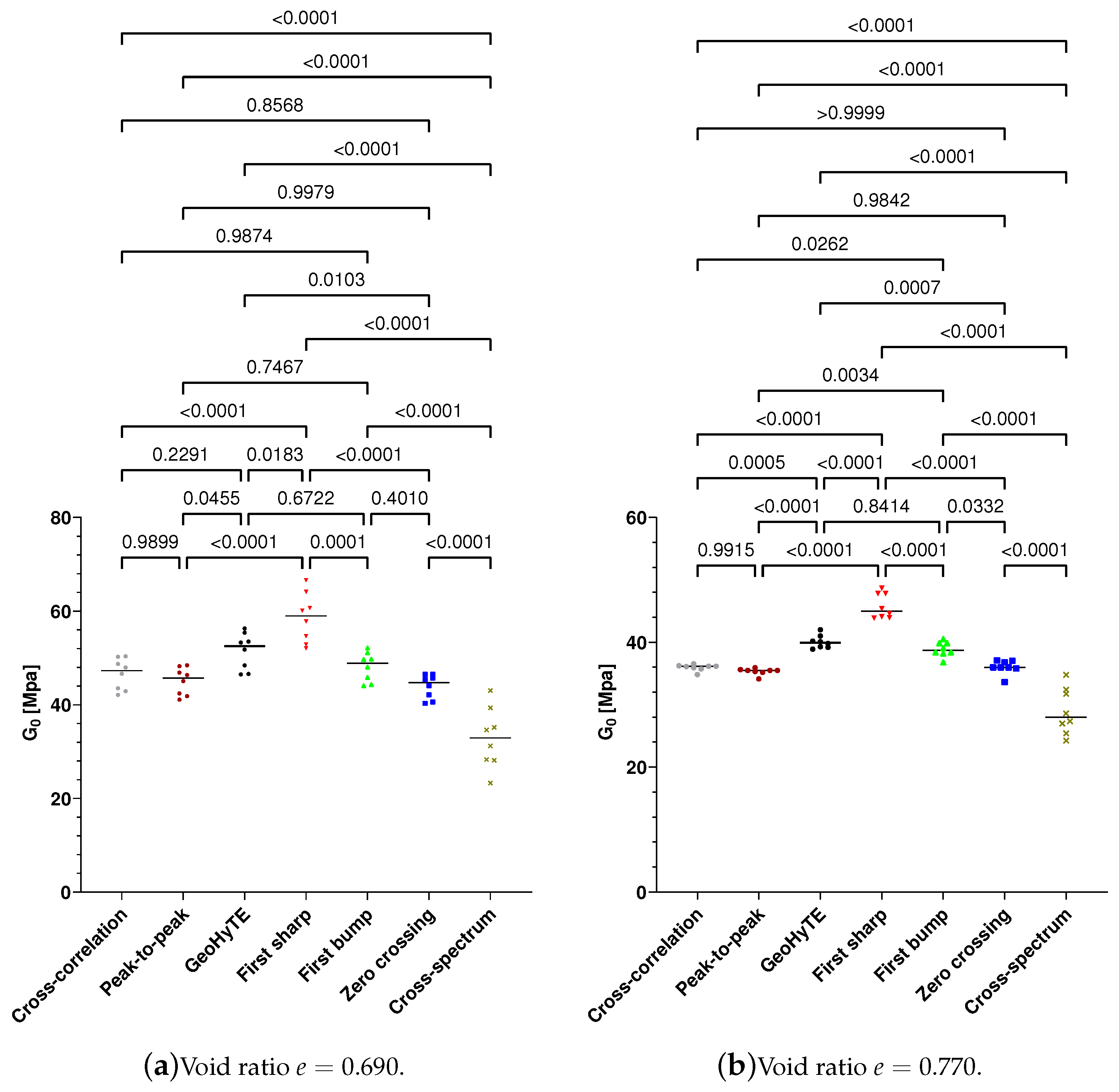
ANOVA tests are utilised to determine whether the means of two distributions are statistically similar. A lower ANOVA metric suggests a lower likelihood of the similarity hypothesis being true. This test is conducted on pairs of distributions, resulting in multiple ANOVA values calculated on all possible combinations the outcomes, as depicted in Figure 21.

The ANOVA tests yield consistent conclusions for both void ratios. The means of the cross-spectrum and first sharp methods are statistically dissimilar to all other interpretation techniques. GeoHyTE is statistically not dissimilar to the first bump technique and, in the $e=0.690$ case, to the cross-correlation method. The pairs (cross-correlation + first bump) and (zero crossing + peak-to-peak) are statistically very similar in the $e=0.690$ case. In the $e=0.770$ case, cross-correlation, peak-to-peak, and zero crossing methods are also very similar.

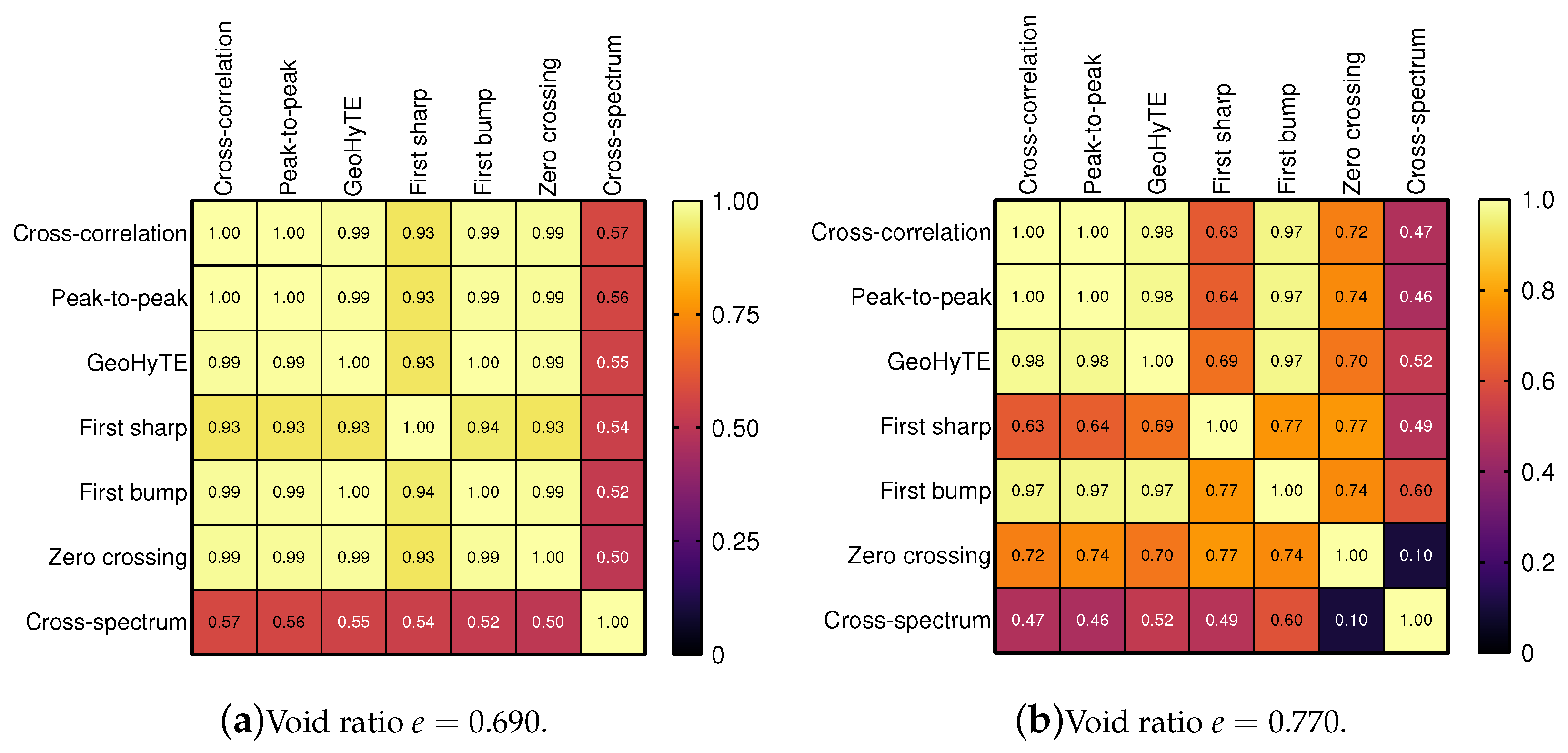
The correlation test assesses whether the readings obtained from one interpretation method exhibit a linear relationship with those obtained from another interpretation method. Unlike the ANOVA test, which provides information on the absolute magnitude of shear modulus values, the correlation test focuses on their relative magnitudes. A higher correlation indicates that the shear modulus values from the two methods are more closely aligned. Figure 22 presents the correlation values between different interpretation methods.

Overall, there is strong correlation between all pairs of interpretation techniques, except for the cross-spectrum method. The shear modulus values obtained with the cross-spectrum method are notably smaller than those obtained with other methods and show significant variance. This trend has been noted by previous researchers, for instance, in references [6,12].

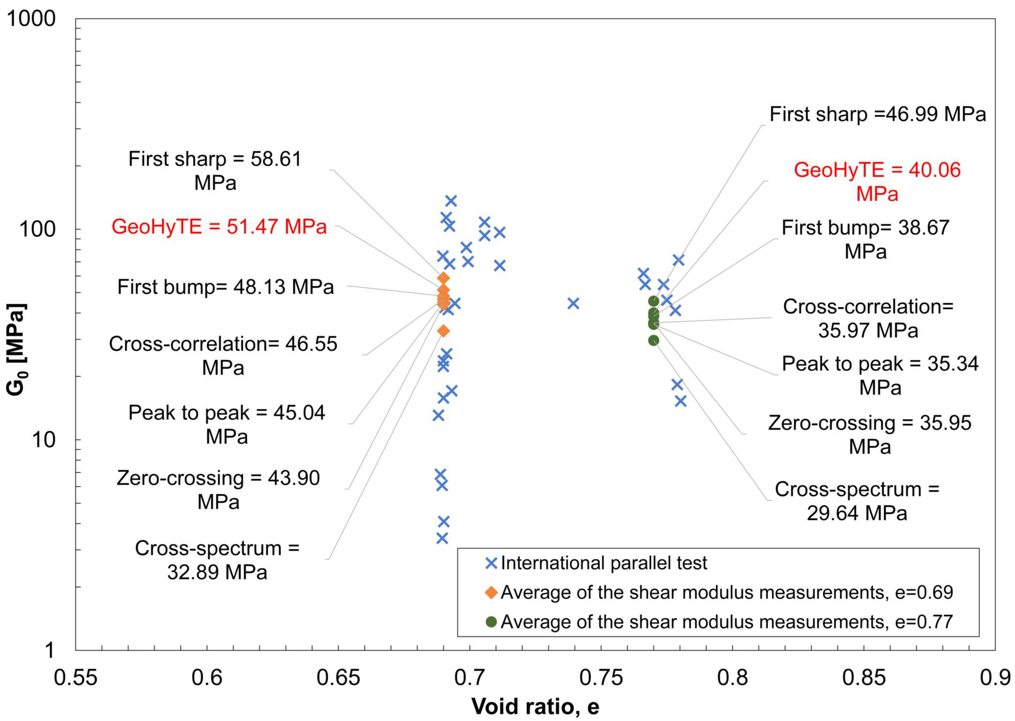
Finally, a comparison is made between the average values of the shear moduli obtained with each interpretation technique and those reported in the International Parallel Test. The results are presented in Figure 23.

The shear moduli reported here generally align well with the bulk of readings documented in the International Parallel Test, except for those obtained with the cross-spectrum method. Predictions from GeoHyTE appear slightly more favourable compared to mainstream techniques like cross-correlation and peak-to-peak distance. However, this improvement is not statistically significant, as indicated by the ANOVA test, so this finding should not be generalised.

5. Robustness of GeoHyTE Predictions

As opposed to most conventional interpretation techniques, the model updating technique encoded into GeoHyTE is objective and physically consistent. Objectivity means that the interpretation of the same output signal should yield similar results independently of the analyst, provided that some simple routine is properly executed. Physical consistency is grounded in the use of a finite element model representative of the experiment, which enables the correlation of two signals of the same nature, namely the output signal obtained in the lab and the output signal obtained with the model. This is an important difference compared, for instance, with the cross-correlation technique presented in Section 2.1.4, which is also objective but physically inconsistent since it correlates signals of different natures (input and output).

However, the objectivity can be compromised if the final value of the shear modulus is influenced by the (subjective) choice of the first estimate of the arrival time. This is a typical risk of conventional extremum finding techniques which are unable to distinguish between local and global extrema. In reference [15], the authors showed that the fixed-point technique has a very large attraction basin, meaning that it converges to the global maximum correlation for a very wide choice of starting points and very fast convergence. The study of the solution convergence presented in Section 5.1 corroborates that conclusion and, in addition, offers the mathematical explanation of this behaviour.

Also, the physical consistency may be hindered by poor finite element results, especially given the complexity of the mechanical behaviour of porous materials and the relatively high excitation frequencies. This issue is studied in Section 5.2, where it is shown that the convergence value of the shear modulus is very insensitive to imperfect finite element results obtained, for instance, using very coarse meshes and poor approximation bases.

5.1. Robustness to Erroneous Initial Shear Modulus Estimate

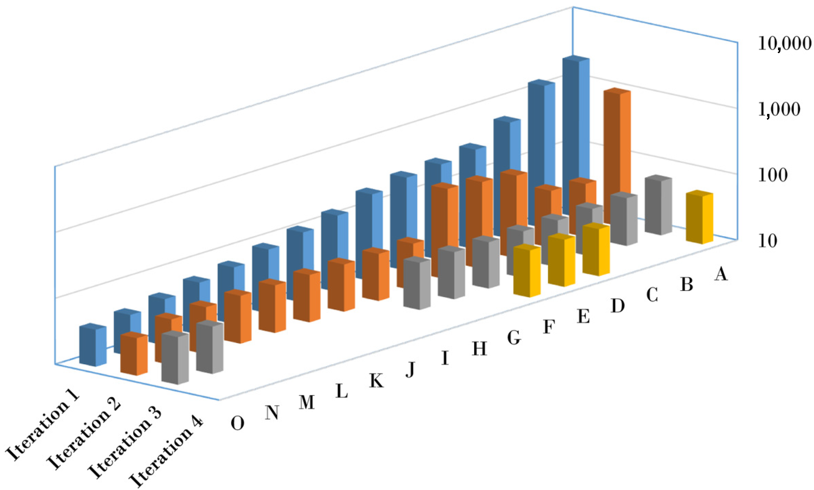
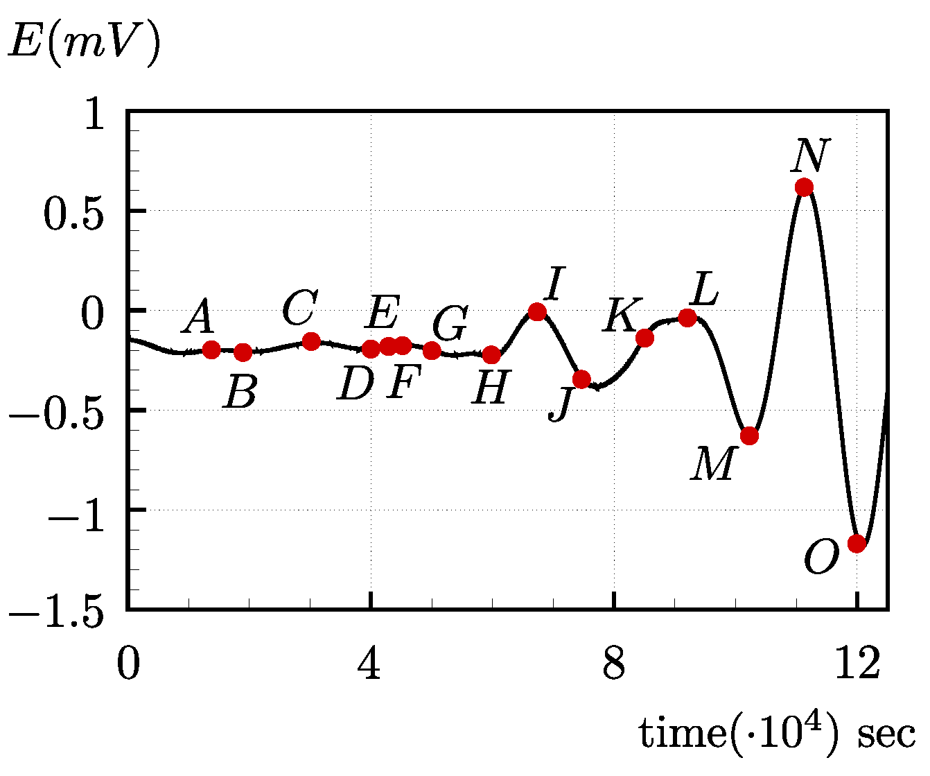
We consider, again, the testing setup used in Section 4.2 to illustrate the conventional and model updating interpretation techniques. To evaluate the convergence properties of the fixed-point method implemented in GeoHyTE, the iterative process is performed starting from 15 points within the correlation window, as shown in Figure 24.

The objective of the study is not only to show the ability of GeoHyTE to converge to consistent solutions, but also to sketch a plot of the update function (5) in order to study the mathematical grounds of this ability. Therefore, not all initial points in Figure 24 are practically reasonable. For instance, points A to G precede all significant oscillations in the output signal and therefore their choice as plausible arrival times is probably not reasonable. Likewise, point O is posterior to large amplitudes in the output signal, so the arrival of the shear wave probably occurs earlier. Nevertheless, the fixed-point iterative process is convergent for all starting points, within no more than four iterations. The values of the shear moduli obtained during the iterative processes are shown in

Table 5. Shear modulus convergence for different starting points.

Arrival Time (s)	Point	${\mathit{G}}_0^1$	${\mathit{G}}_0^2$	${\mathit{G}}_0^3$	${\mathit{G}}_0^4$
$1.5\times {10}^{-4}$	A	2321.10	1019.40	66.10	52.90
$1.9\times {10}^{-4}$	B	1446.10	63.90	53.10
$3\times {10}^{-4}$	C	582.20	72.80	52.70
$4\times {10}^{-4}$	D	326.00	179.10	51.30	51.70
$4.3\times {10}^{-4}$	E	282.20	208.30	50.80	51.70
$4.5\times {10}^{-4}$	F	258.10	237.40	50.50	51.70
$5\times {10}^{-4}$	G	209.10	50.80	51.70
$6\times {10}^{-4}$	H	145.40	51.60	51.70
$6.7\times {10}^{-4}$	I	116.30	51.90
$7.5\times {10}^{-4}$	J	92.80	52.10
$8.5\times {10}^{-4}$	K	72.20	52.70
$9.2\times {10}^{-4}$	L	61.70	53.20
$1.02\times {10}^{-3}$	M	50.20	51.80
$1.11\times {10}^{-3}$	N	42.40	49.30	52.00
$1.2\times {10}^{-3}$	O	36.30	36.90	52.40

. It is noted that notation $G_0^i$ designates the shear modulus used in iteration i.

The convergence process is graphically depicted in Figure 25. The vertical axis, where the values of the shear moduli are plotted, is logarithmic to endorse a clearer observation of the convergence patterns. The convergence process is successfully completed for all starting points and the final shear modulus predictions vary between $51.70$ MPa and $53.20$ MPa. The average shear modulus value is $52.20$ MPa and the standard deviation of the predictions is $0.541$ MPa.

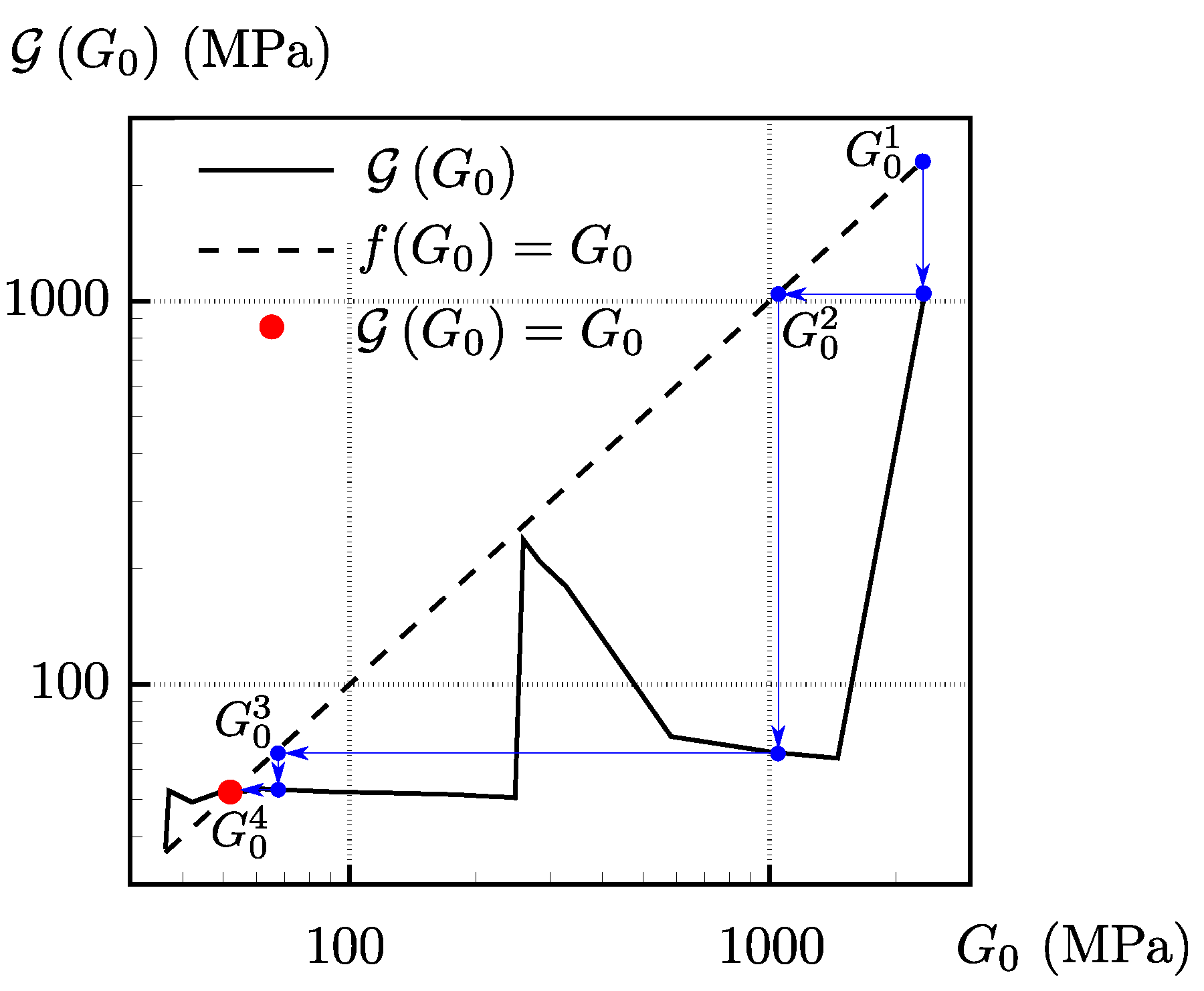
To better understand the mathematical justification of the speed of the convergence process, the update function defined by Expression (5) is plotted with a solid line for 25 values of $G_0$ in Figure 26. The tentative shear modulus at the start of an iteration is represented on the abscissa. The updated shear modulus after the iteration is completed is plotted on the vertical axis. Bots axes are logarithmic. The fixed point axis defined by $f\left(G_0\right)=G_0$ is also plotted with a dashed line.

For reader’s convenience, the iterative process starting from point A (see Table 5) is illustrated with blue arrows in Figure 26. It starts from the tentative shear modulus $G_0^1=2321.10$ MPa which is assumed to lay on the fixed point axis. After the first iteration, GeoHyTE delivers a better approximation of the shear modulus, $G_0^2=1019.40$ MPa, which is, again, assumed to be a fixed point. The process is repeated, yielding, successively, $G_0^3=66.10$ MPa and $G_0^4=52.90$ MPa, with the last point being confirmed as a fixed point within the stipulated tolerance. The fixed point is marked with a red dot in Figure 26.

The fixed point iterative process is convergent if the (absolute value of the) derivative of the update function in the fixed point is less than one. The lower the value, the faster the convergence. For our case, the update function has a single fixed point, as the solid line intersects the fixed point axis in a single point. This is an important advantage of the fixed-point technique implemented in GeoHyTE over conventional correlation maximisation methods. Indeed, the correlation function is known to have multiple local extrema [15], but a single fixed point is identified in this study. This explains why (roughly) the same fixed point is found regardless of the starting point of the iterative process, while the presence of local correlation extrema means that a conventional maximisation algorithm cannot be guaranteed to reach the global maximum. Moreover, the update function in the fixed point is nearly horizontal, meaning that its derivative is significantly inferior to one, which explains the convergence speed of the iterative process.

5.2. Robustness to Imperfect Finite Element Solutions

The problem analysed in Section 4.2.3 is solved here using inadequate mesh and basis refinements to assess the consequence of erroneous finite element solutions on the output of the iterative model updating process. The algorithmic parameters chosen for the reference setup described in Section 4.2.3 are adopted to endorse direct comparison. The first tentative arrival time is $t_{arr}=0.920$ ms and the correlation window is taken until after the largest oscillation in the output signal, at $t_{corr}=1.220$ ms.

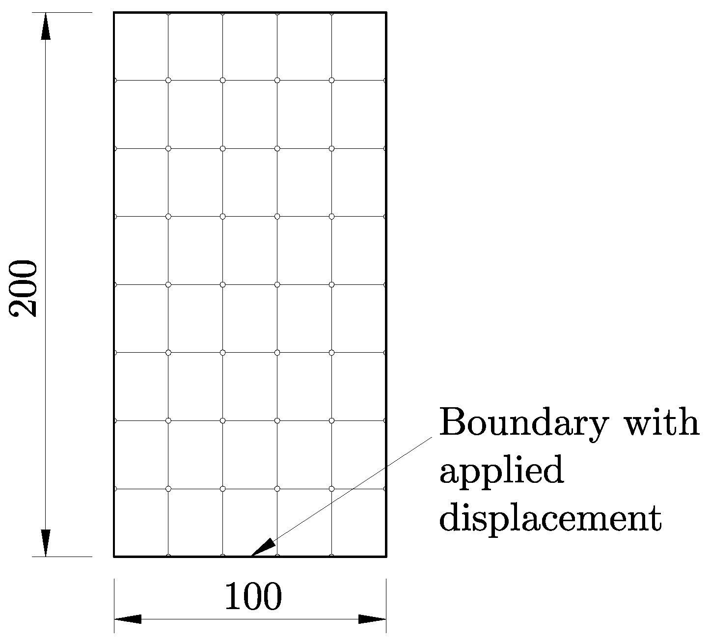
The finite element model is constructed using the purely rectangular geometry presented in Figure 27, meaning that the transmitter bender element is not explicitly included in the model. The domain is discretised into 40 rectangular elements of equal dimensions, with no additional refinement in the zone with large gradients of the solution. The elements are 20 mm by 25 mm in size. Very coarse approximation bases are adopted in the finite elements and on their essential boundaries. For the former, Bessel bases of the third order are adopted, while for the latter, linear shape functions are used. The total number of degrees of freedom of the model is 1348. For comparison, it is noted that the reference model presented in Section 4.2.3 features 198 finite elements and 14296 degrees of freedom. The computational time for the reference model is 10–12 times higher than for this model.

Because the transmitter bender element is not included in the model, the shear wave is triggered by the lateral (tangential) displacement of the boundary located in the middle of the bottom side of the domain, as indicated in Figure 27. The lateral displacement has a parabolic variation in the horizontal direction, null on the extremities of the boundary and equal to ${10}^{-6}$ m in the middle. All other exterior boundaries are unconfined in the tangential direction and fixed in the normal direction.

As expected, the finite solution obtained in this way is of poor quality. The horizontal displacement time–history at the tip of the receiver is presented with a solid line in Figure 28, overlapping the solution obtained with the fine refinement (dotted line). The displacement values are normalised to the maximum absolute displacement of the refined solution.

In Figure 29, the horizontal displacement solutions over the whole domain are plotted at instants $t_1$ to $t_6$, identified in Figure 28. Note that these are the same instants used to plot the solutions for the refined model in Figure 20.

It is clear that the finite element solution obtained with the coarse model is far worse than that obtained with the finer refinement, especially in the bottom region, where the solution gradients are large. Displacement fields are markedly discontinuous between adjacent elements in Figure 29a,b (the mesh was overlapped to stress the internal boundaries), and spurious solution oscillations are also identifiable in the other plots. However, they tend to diminish over time as the gradients of the fields decrease, meaning that the output signal is only slightly affected by these issues (see Figure 29d,f). This is a consequence of the fact that the problem is solved in a single time step [14], meaning that the discontinuity of the solution at a certain time is not transmitted to the next time step as an initial condition. The iterative model updating process converges in only two iterations to shear modulus estimate $G_0=52.30$ MPa, consistent with the value obtained for the reference case, $G_0=53.20$ MPa.

6. Conclusions

GeoHyTE is a new computational toolbox for the automatic shear modulus extraction from the output signal provided by bender element sensors. GeoHyTE searches for the shear modulus that maximises the correlation between the output signals obtained experimentally and using a finite element model. The hybrid-Trefftz finite elements implemented in GeoHyTE are ideally suited to highly transient problems involving large solution gradients, as typical for bender element tests. They are nearly wavelength-insensitive, meaning that the well-known requirement of calibrating the leading dimension of the finite elements to cover at most $1/6$ of a wavelength needs not be observed. For this reason, good shear modulus predictions can be obtained using very coarse finite element models.

GeoHyTE was thoroughly tested and validated using a well-known granular geomaterial, and its predictions were compared with all mainstream interpretation techniques. The shear moduli produced by GeoHyTE compare well with other time domain interpretation techniques and with the bulk of the results reported in an International Parallel Test that was used as a benchmark. The procedures built into GeoHyTE can be used for clays, too. However, since clays typically have very low permeability, the seepage between solid and fluid phases is generally neglected and they are modelled as single-phase materials. In this sense, using hybrid-Trefftz elements based on the Biot’s theory is not economical from a computational perspective. Future releases of GeoHyTE will include finite elements for single-phase media which will be able to model clays at a lower computational price.

GeoHyTE is highly insensitive to the starting point of the maximisation process and able to converge to a global maximum of the correlation despite the presence of local extrema. Moreover, the derivative of the (single) fixed point of the update function is close to zero, meaning that it is an attractor and the convergence is very fast. The maximum number of iterations needed to converge was four, despite the vast differences between the starting points essayed in this study. As opposed to most conventional techniques used for the interpretation of bender element tests, the procedure implemented in GeoHyTE is objective (as it does not depend on the experience of the analyst) and physically consistent (as it correlates signals of the same nature, obtained taking into account the physical features of the experiment).

GeoHyTE is user-friendly, featuring graphical user interfaces for all phases of the definition of the model, and highly flexible, as it enables the use of localised basis refinements, meaning that different refinements of the domain and boundary bases can be defined on different elements and essential boundaries. It uses implicit parallel processing techniques to improve its computational efficiency and outputs detailed descriptions of all fields at every iteration, which can be used to visualise the solutions after (and even during) the execution. A beta version of the software is available to the scientific community upon request [20].

We believe that this paper will enable GeoHyTE to become a mainstream signal interpretation technique for bender element sensors.