Fast Algorithm for High-Throughput Screening Scheduling Based on the PERT/CPM Project Management Technique

Abstract

High-throughput screening systems are robotic cells that automatically scan and analyze thousands of biochemical samples and reagents in real time. The problem under consideration is to find an optimal cyclic schedule of robot moves that ensures maximum cell performance. To address this issue, we proposed a new efficient version of the parametric PERT/CPM project management method that works in conjunction with a combinatorial subalgorithm capable of rejecting unfeasible schedules. The main result obtained is that the new fast PERT/CPM method finds optimal robust schedules for solving large size problems in strongly polynomial time, which cannot be achieved using existing algorithms.

1. Introduction

High-throughput screening (HTS) systems are intelligent robotic cells widely used in pharmaceutical and biomedical research to analyse new chemicals, discover new drugs, and detect new viruses [1,2]. Advances in human genomics, along with the need to discover new drugs and detect viruses, have driven requirements for testing of an increasing number of biochemical compounds. The primary goal of HTS is to detect and identify lead compounds that significantly affect the target of the analysis under study. There are typically thousands of samples that need to be processed in a very short time. While HTS is defined by the number of compounds tested, ranging from 10,000 to 100,000 per day, ultra-HTS is characterized by the screening of in excess of 100,000 compounds per day [3,4]. These substances for screening are fed into the robotic cell on microplates and then transported by the robot between workstations according to the screening process.

Robots and robotic cells for HTS range widely from simple automatic dilution devices to complex fully automated workstations in which robots perform a variety of functions from sample dispensing to data collection, allowing for significant increases in screening speed. However, conversion to an automated format introduces certain difficulties that affect the design of the assay in practice. In particular, some operations are relatively difficult to automate, such as removing debris, washing wells, and separating substrate from product. Additionally, the more steps required for analysis, the more difficult it is to automate, control, and schedule HTS operations. The purpose of this paper is to use advanced operations research techniques and scheduling theory to optimally schedule the HTS process and maximize cell performance.

A typical HTS cell includes a fixed set of workstations performing preparation, deposition, liquid dispensing, reading and analyzing, and incubation operations. The microplates pass through the workstations sequentially in the same order in such a way that each microplate can re-enter the corresponding workstations (in scheduling theory, this type of process is called a re-entry flowshop).

The microplate processing time of a workstation is the minimum time that a microplate must remain on a workstation before the robot moves it to the next workstation. While a microplate remains on the workstation, the next microplate cannot enter it; in scheduling theory, this condition is called blocking. The goal is to find a cyclic schedule of robot moves that minimizes cycle time, i.e., maximizes cell productivity. From the point of view of scheduling theory, the scheduling problem under consideration is a cyclic single-robot, multiple-machine flowshop scheduling problem with blocking and re-entry [5,6,7]. An HTS system with an optimal schedule can minimize the overall screening time, maximizing the throughput and hence reducing associated costs and enabling diagnosis of diseases and rapid discovery of new drugs [8,9,10].

The scheduling problem under consideration has a complex combinatorial structure and is difficult to solve. In recent decades, several popular methods, such as mixed integer programming (MIP), Petri nets, max-plus algebra, greedy heuristics, and genetic algorithms, have been used to find optimal schedules for HTS processes. However, many existing methods have prohibitively high exponential computational complexity in the worst case and therefore cannot be guaranteed to quickly find the optimal solution for large problem instances.

This raises the question of whether there is a method for such scheduling problems that can find the optimal schedule for arbitrary data in polynomial time. In what follows, we give a positive answer to this question; namely, we develop a new efficient and practical version of the PERT/CPM project management method to solve this problem. To demonstrate the validity and practical usefulness of the new method, we focus on the theoretical and numerical analyses of the HTS process for enzymatic assays. Although the scheduling problem under consideration is complex and NP-hard, we solve it efficiently using the proposed method if the number of screening operations is limited, which is a condition usually encountered in practice [11,12].

This result complements the original studies of Oke et al. [11,13] and Wu et al. [12,14], who used mixed integer programming and resource-oriented Petri nets, respectively, to model, analyze, and solve the HTS scheduling problem for enzymatic assays. The proposed PERT/CPM method works in conjunction with the prohibited intervals subalgorithm [15], which weeds out unfeasible solutions and finds the optimal schedule in strongly polynomial time (in the number of operations m), O(m³ log m), which, as far as we know, cannot be achieved using existing algorithms. This worst-case polynomial complexity is a major advantage over the existing HTS scheduling algorithms mentioned above. Moreover, our solution method can not only produce a single optimal solution such as an MIP model or a Petri net; rather, it can generate a whole set of different schedules, each of which is optimal, and any of them can be selected by decision makers in accordance with their purpose and requirements. Finally, unlike the aforementioned MIP algorithm in [11], the proposed method ensures that the resulting optimal schedules remain robust (stable) under relatively large variations in cycle time; this property of stability differs from robustness in Petri nets (see, e.g., [3,16]), and will be explained in detail in Section 4.

The rest of the paper is organised as follows. The next section describes the problem. Section 3 presents previous works and a literature review. Section 4 finds the best 1-cyclic robot route and describes the parametric PERT/CPM project management method for determining the minimum 1-cyclic time; the rest of this section describes the combinatorial subalgorithm, working in combination with the PERT/CPM method, and provides a resulting optimal 2-cyclic schedule which is robust and obtained in polynomial time. Section 5 concludes the article.

2. Description of the Problem

As explained in the previous section, the HTS system is a robotic cell in which substances to be screened are supplied to the cell on microplates, and then the microplates are transported by the robot between workstations according to the screening process flow. To demonstrate the validity and practical usefulness of the scheduling method developed below, this paper focuses on the theoretical and numerical analyses of the HTS process for enzymatic assays.

Enzymatic assays are one of the typical applications of HTS systems. A typical HTS system for an enzymatic assay includes the following basic workstations [11,12,13,14]:

• Cytomat2C, a microplate hotel designed to prepare microplates for screening.
• Multidrop-384, a dispenser for dispensing liquid substances into the wells of microplates.
• The Envision device, a reader for identifying and analyzing changes occurring in the biochemicals being analyzed.
• Teleshake, a device that maintains the necessary environment to allow biochemical substances in the wells of a microplate to incubate.
• A storage center, which holds the microplates for screening.
• The transportation robot SCARA, used for delivering microplates among the above devices to performing the specified screening procedures.

The microplates enter the robotic cell periodically, and the robot SCARA transports all of the microplates between the workstations. There is an auxiliary device, separate from the robot, that automatically delivers the microplates between the storage center and the Cytomat2C, such that the system can continuously operate without interruption. In the screening process under consideration, each microplate passes through workstations in the same predefined technological sequence, as follows: Cytomat2C → Multidrop-384 → Envision → Teleshake → Envision → Cytomat2C. In what follows, this technological sequence of workstations is denoted by S = (M₀, M₁, M₂, M₃, M₂, M₀), where M_i, i = 0, 1, 2, 3, 2, 0, are the designations of the respective workstations.

In Figure 1 below we have plotted a PERT graph that depicts a typical HTS screening process and its actual timing characteristics, as presented in [11,14]. The operations shown in this figure are repeated for each individual microplate. This graph and Figure 2 clearly show that the Cytomat2C and Envision workstations perform two operations during each cycle in the technological sequence.

Nodes represent repetitive operations performed by workstations during the screening of each microplate. Capital letters within nodes identify workstations as follows: S for Storage Centre, C for Cytomat2C, M for Multidrop-384, E for Envision, and T for Teleshake. The numbers inside the nodes indicate the required time (in seconds) for the corresponding activity on the workstation. The arcs between nodes and the corresponding weights of the arcs denote the robot’s delivery operations and their durations (in seconds), respectively. The arcs between the Storage Centre and the Cytomat2C, and between the Cytomat2C and the Storage Centre, which are both of zero length, represent the delivery operations performed by the auxiliary transportation device.

Next, for the convenience of the readers, we present a Gantt chart in Figure 2 to visualize how this data are used to determine the robot’s path and movement of microplates between workstations in space and time. This chart will be constructed and used later, in Section 4, using a general PERT/CPM-based method to find the optimal cyclic schedule that minimizes cycle time. This cyclic schedule, with a period of 200.5 s, is shown in Figure 2.

In the Gantt chart in Figure 2, the following notation is used: workstations 0, 1, 2, and 3 denote Cytomat2C, Multidrop-384, Envision, and Teleshake, respectively. The abscissa axis corresponds to time. The robot’s movement is shown with a red dotted line. The numbers in the figure indicate the time the robot arrives at and leaves the corresponding workstations. The first robot’s cycle begins at time t = 0, when the robot picks up a screen-ready microplate, labeled MP₀, from workstation 0 (Cytomat2C), then moves this microplate MP₀ to workstation 1 within 19 s. The robot then visits workstations in the following order: the void robot moves (without a microplate) to workstation 2 (next in the sequence S) → the robot moves with microplate MP₋₂ (which starts two cycles before microplate MP₀) to workstation 0 → the void robot moves to workstation 1 → the robot moves, loaded with microplate MP₀, to workstation 2 → the robot moves with microplate MP₀ to workstation 3 → the robot moves with microplate MP₋₁ to workstation 2 → the void robot moves to workstation 0, where the robot waits for 35 s and completes its 1-cyclic route at t = 200.5 s. The total processing time for the microplate MP₀ is significantly longer and amounts to 506 s. It begins at time t = −32 (not shown in Figure 2), when this microplate is delivered by the auxiliary device to workstation 0, and ends at time t = 474 s, when microplate MP₀ is returned by the auxiliary device to the storage center, which occurs during the third cycle of the robot. The processing life of microplate MP₀ is indicated by a bold blue line with small triangles.

The symbol MP_−k (k = 1, 2, …) denotes a microplate that enters the screening system k periods (cycles) before MP₀. It can be seen that two adjacent instances of the corresponding operation in workstation 3 (Teleshake) for two adjacent microplates intersect in time. In order not to overload Figure 2, operations from S to C and from C to S visible in Figure 1 are not shown in Figure 2. We denote the sequence of operations performed on the workstations as O = (O₀, O₁, O₂, O₃, O₄, O₅), which means that operations O₀ and O₅ are performed on workstation M₀ (Cytomat2C), operation O₁ is performed on workstation M₁ (Multidrop-384), operations O₂ and O₄ are performed on workstation M₂ (Envision), and operation O₃ is performed on workstation M₃ (Teleshake). In this notation, the symbols R = (O₀, O₄, O₁, O₂, O₃) denote a periodically repeating sequence of completed operations, which uniquely determines the cyclic route of movement of the loaded robot.

The Gantt chart shows that four identical microplates are sequentially introduced into the system by the robot at times 0, 200.5, 401, and 601.5 s, respectively. The bold horizontal lines show the processing operations at the workstations, and the thin dotted line shows the route of the robot between the workstations. For the reader’s convenience, to distinguish between operations on different microplates, their horizontal lines are depicted in different colors and use indicators represented by small triangles, squares, and diamonds, respectively. Figure 2 clearly shows that the Cytomat2C and Envision workstations perform two operations (on different microplates) during each cycle in the process sequence.

Remark. We will study the scheduling problem under consideration from the point of view of PERT/CPM project management. The Project Evaluation Review Technique (PERT) and the Critical Path Method (CPM) are often used by project managers and decision makers to break complex, large-scale projects into individual activities, identify the logical dependencies between them, and then manage them to minimize the overall project cost and time [17,18]. In summary, PERT and CPM are operational research and scheduling techniques with important advantages in practice, including clarity, user-friendliness, rigor and flexible mathematical modeling, and computational efficiency. These techniques are widely used in many industries, sectors, and services [18,19]. The PERT/CPM method is successfully used in this study to solve the practical problem considered in [11,14], and, as we will show below, this mathematical model has significant computational and practical advantages over existing MIP and Petri net methods.

In this section, we recall several basic definitions in scheduling theory [5,6,20,21]. A cyclic schedule can be defined as a schedule that repeats itself at fixed intervals of time; these fixed intervals are called cycle time. If k microplates enter and leave the robotic cell during a cycle, such a schedule is called a k-degree cyclic schedule, or a k-cyclic schedule.

It is required to find a schedule of robot moves that minimizes the average cycle time T_avr, and thus maximizes the productivity of the cell.

During each cycle, the robot can serve different microplates, which start the screening process at times … −T, 0, T, 2T, …, respectively. The Gantt chart in Figure 2 illustrates the optimal 1-cyclic screening schedule which will be obtained below. The durations of operations at the workstations for the benchmark problem in [11,14] are the same as shown in Figure 1. The detailed calculation of this schedule will be presented in Section 4.

Let us formulate the HTS cyclic problem in standard scheduling theory terms. Denote by M₀, M₁, M₂, M₃ the workstations Cytomat2C, Multidrop-384, Envision, and Teleshake, respectively. In the screening process under consideration, the microplate passes through the same predetermined technological sequence of workstations, denoted by S, that starts from workstation M₀ and continues as follows: S = (M₀, M₁, M₂, M₃, M₂, M₀), where workstations M₀ and M₂ are re-entered.

Recall that the sequence of operations performed on the workstations is denoted O = (O₀, O₁, O₂, O₃, O₄, O₅).

The following conditions are imposed:

• The time, denoted p_k, that a microplate spends on a workstation before the robot moves it to another workstation is unknown, but the lower bound, l_k, of this time is known in advance.
• Workstations M₀, M₁, M₂, and the robot can only hold one microplate at a time.
• The number of microplates simultaneously processed at workstation M₃ can be greater than one. Let us denote by β the maximum number of microplates that can be simultaneously served at workstation M₃. The capacity β of the Teleshake is flexible; that is, β is a variable whose optimal value must be found.

Each operation O_k, k = 0, 1, …, 5, of the processing sequence O is characterized by the following parameters:

• p_k, the processing time of operation O_k, k = 0, 1, …, 5;
• d_k, the time required for a robot to deliver a microplate from a workstation performing operation O_k to the next workstation in technological sequence S, k = 0, 1, …, 5;
• l_k, the lower bound for the processing time of operation O_k, i.e., p_k ≥ l_k, k = 0, 1, …, 5.

In this model, all p_k are assumed to be unknown (decision variables) while the l_k and d_k values are given input data. The time required for an unloaded robot to move from one workstation to another is considered negligible.

In Section 4, we present a fast HTS scheduling algorithm that solves the problem under study using two coupled algorithms. The first algorithm is a parametric PERT/CPM project management algorithm, and the second is a modification of the existing prohibited intervals method. Among all available robot paths, the proposed algorithm selects the path with the minimum cycle time.

For reader convenience, each step of the general algorithm proposed will be accompanied by a numerical example, which is generated from the data of the actual screening process of an enzymatic assay as discussed in [11,14]. The relevant timing parameters are presented in Figure 1 and Figure 2. In the notation introduced above, these time parameters are as follows (in seconds): l₀ = 32, l₁ = 20, l₂ = 54, l₃ = 210, l₄ = 54, l₅ = 34; d₀ = 19, d₁ = 23, d₂ = 20, d₃ = 20, d₄ = 20.

3. Related Work: Literature Review

Scheduling theory is a widely discussed research topic in operations research and industrial engineering [5,6,7,20,21,22]. However, since HTS is a relatively new technology, its scheduling problems have not yet been extensively studied. There is presently not much literature on HTS scheduling algorithms, despite the fact that they are clearly interesting from a theoretical point of view and applicable in practice.

It was in the 1970s and early 1980s that the components that make HPS technologies possible came together. These were robots and small-scale servo-powered robotic devices, microplates, and apparently, most importantly, personal computers. In 1974, this technology was first used for enzyme-linked immunosorbent assay (ELISA) in London and at the Centers for Disease Control (USA) [23].

In early studies, heuristic and approximation methods such as genetic algorithms were proposed to solve the HTS scheduling problem [1,24,25]; however, they could not guarantee an optimal solution. Thus, the applicability of these methods is limited. In one of the first papers on the topic that we are aware of [4], the authors presented a computer-integrated model incorporating characteristics of HTS scheduling problems for different assays. They observed that, as with most hard scheduling problems, there are no efficient algorithms for finding optimal solutions in HTS; hence, they proposed the use of heuristic procedures and genetic algorithms, which had become known for their applicability in flowshop and jobshop problems in scheduling theory several decades earlier.

In [24,26], the authors focused on creating an optimal HTS schedule exploiting cyclic Petri net models. When defining the variables in their model, they used the starting and ending events of activities. This way of defining discrete time nodes was easy to implement in the scheduling model. Another study [27] was a continuation of previous work [26], and was also based upon Petri net concepts with the aim of determining a globally optimal schedule for HTS systems. In addition, these authors extended their model to include the hierarchical nesting of cycles.

In paper [16], the authors modeled the HTS system using a dioid algebraic approach and applied max-plus algebra to the cyclic HTS. In max-plus algebra, the addition and multiplication operations of classical arithmetic are replaced by the max and addition operators, respectively. The scheduling problem was then transformed into the problem of calculating a feedback controller that could function correctly in the presence of variations, disturbances, and delays. In [3], the author studied timed event graphs with constraints, and modeled systems with nested schedules. To apply his findings, he used the proposed method to analyze a real HTS system, and found an optimal schedule. Extending the dioid and Petri net approaches, the authors of the mentioned works [24,25,26,27] used mixed integer programming formulations to schedule real HTS systems.

An important step forward in the analysis and practical use of the considered HTS scheduling problem was made in recent studies [11,12,13,14] that significantly developed the mixed-integer programming (MIP) and resource-oriented Petri nets approaches, respectively, to model, analyze and solve the considered problem. The study in [11,13] was motivated by the practical problem of automated testing for viruses and new drugs using HTS. The authors examined in detail how scheduling screening activities in a real-world HTS system affects its efficiency, throughput, operating costs, and screening quality. The purpose of that work was to minimize the total screening time and to study the features of the screening process that guarantee the optimal schedule. These authors developed innovative and comprehensive mixed-integer programming models that efficiently computed optimal cyclic and non-cyclic schedules for multi-microplate screening with several real-world biomedical applications, namely the drug discovery process of screening enzymatic assays and the general SARS-CoV-2 detection process. The authors convincingly showed that their MIP algorithm can significantly reduce screening time compared to some commercial software products. Using a comprehensive MIP model, they found the optimal 2-cyclic schedules for enzyme assay screening. However, finding a solution in the MIP model for real cases of the problem may be inefficient, because the computation time for solving the MIP problem depends exponentially on the number of integer variables in the model, limiting the practical application of such methods for large-scale cases.

The question arises whether there is a polynomial algorithm for solving this problem. This is a challenging issue that has been considered in papers [12,14], in which the HTS system was modeled with complex and detailed resource-oriented Petri nets. Using this model, the authors of these studies found and analyzed the necessary and sufficient conditions under which a feasible cyclic schedule may exist and obtained an optimal schedule for the problem under consideration. Although they did not explicitly disclose the complexity of their algorithm, their work clearly represented a valuable breakthrough from a theoretical perspective and showcased an important practical application of HTS technology. Our article can be seen, in a sense, as a complement to this research. While the algorithm in [12,14] successfully finds a single optimal cyclic schedule for the problem under consideration, we will show that the proposed PERT/CPM-based algorithm discovers and discloses a whole set of optimal and robust schedules for that problem.

4. The Parametric PERT/CPM Method for Finding the Optimum Schedule

In this section, we present a fast scheduling algorithm that solves the problem using two conjugated algorithms, A and B (see Figure 3). The main algorithm, denoted A, is the PERT/CPM project management method, which considers the case where the robot’s route is fixed, and each processing time lies within a specified time interval known as a time window. We also consider the case where the number of processing operations is limited by a small constant, as is the case in practice in enzymatic assays. In this case, the total number of possible robot routes is a reasonable fixed number, and the proposed algorithm begins with generating all available robot routes. Then, the first algorithm can alternately process all available robot routes, one after another, and find, among them, the route that produces the minimum-time 1-cyclic schedule. For this purpose, we use and extend the parametric PERT/CPM algorithm on a directed weighted graph, which had been previously developed by the authors in [21]; the latter algorithm is modified to accommodate the specifics of HTS, and is described below. This procedure is repeated for each feasible robot route, and then, among all the obtained pathfinding solutions, the algorithm A selects the 1-cyclic route with the minimum cycle time.

At the output of the first algorithm A we obtain the following results: (i) the optimal 1-cyclic robot path, and (ii) the optimal values of the processing times p_k and the variable β that satisfy the technological constraints of the process, as detailed below.

Next, we introduce a second subalgorithm, denoted Algorithm B, which takes as input the optimal processing times p_k of all screening operations provided by the aforementioned PERT/CPM subalgorithm A and finds a set of optimal 2-cyclic schedules. Note that 2-cyclic schedules are generally more efficient than 1-cyclic schedules, and have the following additional advantages: (1) their optimal average cycle time is usually strictly less than the optimal 1-cyclic time, and (2) the resulting set of different 2-cyclic optimal schedules (with each one having possibly different component lengths, but the same average cyclic time) allows us to obtain a robust problem solution. To do this, we modify and use the above-mentioned prohibited intervals method (PIM) from our previous work [15]. Using real numerical data from [11,14], we apply the combined PERT/CPM/PIM algorithm and efficiently solve the considered scheduling problem in polynomial time with respect to the number of operations.

Let us start by describing how we generated all 1-cyclic robot routes. Recall that in the problem formulation in Section 2, it was stated that the robot SCARA moves microplates between four available workstations M₀, M₁, M₂, and M₃, which are the Cytomat2C, Multidrop-384, Envision, and Teleshake workstations, respectively. The sequence of these movements is uniquely determined by the sequence of moments of completion of the five following operations (O₀, O₁, O₂, O₃, O₄). Thus, the considered HTS system has 4! = 24 different robot routes, which we denote by R = (O₀, O_[1], O_[2], O_[3], O_[4]). Obviously, these routes are determined by permutations of the numbers 1, 2, 3, and 4. The route R = (O₀, O₁, O₂, O₃, O₄) is trivial. Thus, the general scheme of the solution procedure is as follows: we first need to consider the 23 remaining routes one by one, then solve the PERT/CPM problem for each robot route, which is presented in the next subsection, and finally select the solution with the minimum cycle time T. In fact, as noted in [14], the specific input data of the enzymatic assay screening process can significantly reduce the number of possible robot routes to be tested.

4.1. Description of the PERT/CPM Algorithm A

This algorithm considers the case where the processing times of operations are flexible and bounded by their low bounds. In addition, the time required to complete the sequence of operations in the HTS system is limited by the specified screening time constraints, which will be presented below. We show that for any given robot route, this problem reduces to the parametric critical path problem, which is a well-solvable special case of a general linear programming problem. Unlike linear programming, the parametric critical path algorithm is executed in a time that is strongly polynomial in the number of operations.

Consider a 1-cyclic robot route, and let T be its (unknown) cycle length. The completion time of operation O_k performed in interval [0, T), k = 0, 1, …, 5 is denoted by t_k. Let us take t₀ = 0, i.e., assume that the cycle [0, T) starts when the robot takes a microplate from workstation M₀ (Cytomat2C). The time in the cycle [0, T) when the (next instance of) operation O₀ starts is denoted using t₆. Note that the microplate, having completed its operation O₀ at time t₀ = 0 starts this instance of this operation at time t₆ − T. The cyclic robot route is denoted using R = (O₀, O_[1], O_[2], O_[3], O_[4]). This means that at time t₀ = 0, the robot picks up the microplate from workstation M₀ and moves it to workstation M₁. If operation O_[1] is performed on workstation M₁, i.e., [1] = 1, then the robot waits for operation O₁ to complete at time t₁. If [1] ≠ 1, then the unloaded robot moves to the workstation performing operation O_[1] and waits there for operation O_[1] to complete at time t_[1]. At time t_[1], the robot picks up the microplate and moves it to the next workstation in the screening process sequence S, as defined in Section 2. If this workstation does not perform operation O_[2], then the unloaded robot moves to another workstation that performs operation O_[2]. Similar robot actions are associated with operations O_[2], O_[3], and O_[4]. At time T, the robot takes the next microplate from workstation M₀ and repeats the same steps as in the previous cycle.

We can now reformulate our cyclic scheduling problem as the following special-type parametric linear programming problem P with t₀ = 0 and variables T, t₁, …, t₆ defined for any specific robot route and introduced below:

Problem P: Minimize T

subject to

The robot move constraints:

t_[k] ≥ t_[k−1] + d_[k−1], k = 1, 2…., 5; t _[5] = T.

(1)

The processing time constraints:

p_k = t_k − t_k−1 − d_k-1 ≥ l_k, if t_k > t_k−1, k = 1, 2, 4;

(2a)

p_k = t_k + T − t_k−1 − d_k−1 ≥ l_k, if t_k < t_k−1, k = 1, 2, 4;

(2b)

p₃ = t₃ − t₂ + (β − 1)T − d₂ ≥ l₃, if t₂ < t₃ and t₃ ≠ t₂ + d₂;

(2c)

p₃ = t₃ + β T − t₂ − d₂ ≥ l₃, if t₃ < t₂ or t₃ = t₂ + d₂;

(2d)

p₀ = t₀ + T − t₆ ≥ l₀;

(2e)

p₅ = t₅ − t₄ − d₄ ≥ l₃.

(2f)

Screening time constraints:

t₁ + d₁ + T − t₆ ≤ 152;

(3a)

t₁ + d₁ − t₀ − d₀ ≤ 44;

(3b)

t₃ + d₃ + (β − 1)T − t₀ − d₀ ≤ 369, if t₂ < t₃;

(3c)

t₃ + d₃ + β T − t₀ − d₀ ≤ 369, if t₃ < t₂.

(3d)

Overlapping constraints:

t₆ − t₅ ≥ 0;

(4a)

t₂ ≤ t₃ + d₃, if t₂ < t₄ or (t₂ > t₄ and t₃ > t₄)

(4b)

t₄ ≤ t₁ + d₁, if t₄ < t₂ or (t₄ > t₂ and t₁ > t₂)

(4c)

The robot-move constraints (1) ensure that the robot has enough time to complete all its movements without delay. Inequalities (2a) take into account the case when the operation O_k starts and ends within the cycle [0, T). Inequalities (2b) consider the case where the operation O_k starts in the cycle [0, T) and ends in the next cycle [T, 2T). Inequalities (2c,d) take into account the case where the processing time of microplates at workstation M₃ exceeds the cycle time T. The parameter β determines the number of simultaneously processed microplates at workstation M₃. In the case where t₃ = t₂ + d₂ in inequality (2d), the robot simultaneously unloads the microplate from workstation M₃ and loads the next microplate onto it. Inequalities (2e,f) determine the processing time of operations O₀ and O₅, respectively. Inequality (3a) requires that the interval between the starts of operations O₀ and O₂ does not exceed the specified value of 152 s.

Inequality (3b) requires that the interval between the starts of operations O₁ and O₂ should not exceed 44 s. Inequalities (3c,d) require that the interval between the starts of operations O₁ and O₄ of the same microplate should not exceed 369 s. Constraint (4a) ensures that operations O₀ and O₅ do not overlap in time on workstation M₀. Constraints (4b,c) ensure that operations O₂ and O₄ do not overlap in time on workstation M₂.

At this stage we need to modify the parametric critical path approach originally proposed by the authors in [21]. We reformulate Problem P above as a parametric critical path model as follows. A graph, G_P, is constructed, in which each t-variable in constraints (1)–(4c) corresponds to a node of the graph. Next, each constraint in problem P is presented in the form t_j ≥ t_i + (a + bT), where i, j ∈ (1, 2, …, 6), a is a real number, and b is an integer. To this constraint we associate a directed arc e_ij in the graph G_P leading from node i to node j and having length w_ij = a + bT (see Figure 4). Thus, problem P reduces to the following parametric critical path problem, denoted Problem Q:

Problem Q. For any specific robot route, find the minimum value of parameter T in the constructed graph G_P, such that the graph does not contain cycles of positive length.

The proof of this reduction is given in [21]. The parameter β in (2c,d) and (3c,d), although it expands the problem formulation in [21], does not violate the proof. Note that as soon as a specific robot’s path is chosen and fixed, the logical (disjunctive) conditions in Problem P acquire only one possible outcome; that is, they cease to be disjunctive. As a result, for each fixed robot route, Problem P is transformed into a special type of a linear programming problem, which reduces to a parametric shortest path problem as proven by the authors in [21].

Now we can solve Problem Q for all robot routes repeatedly using the parametric critical path algorithm [21]. This part of the algorithm requires a routine repeated computation of a cycle time in graph G_P for each available robot route, the total number of which is a small constant. Omitting the intermediate routine calculations for each candidate robot’s routes, we obtain the minimum 1-cyclic time T = 200.5, which is obtained for the robot route R = (O₀, O₄, O₁, O₂, O₃) and β = 2. In this case, the constraints (1)–(4) have the following form:

The robot move constraints:

t₄ ≥ t₀ + 19;

t₁ ≥ t₄ + 20;

t₂ ≥ t₁ + 23;

t₃ ≥ t₂ + 20;

t₀ ≥ t₃ + 20 − T.

The processing time constraints:

t₁ ≥ t₀ + 39;

t₂ ≥ t₁ + 77;

t₃ ≥ t₂ + 230 − T;

t₄ ≥ t₃ + 74 − T;

t₀ ≥ t₆ + 32 − T;

t₅ ≥ t₄ + 54.

Screening time constraints:

t₆ ≥ t₁ − 129 + T;

t₀ ≥ t₁ − 40;

t₀ ≥ t₃ − 368 + T.

Overlapping constraints:

t₆ ≥ t₅ + 0;

t₃ ≥ t₂ − 20;

t₁ ≥ t₄ − 23.

The corresponding parametric PERT/CPM graph G_P, which has positive and negative operation durations, some of which may depend on the parameter T, is presented in Figure 4. The nodes in the graph correspond to six operations, O_k, performed in the interval [0, T), k = 0, 1, …, 5. Constraints of type (1) are represented by arcs of length d_k leading from node k to node k + 1; constraints of the form t_i + d_i + T − t_j ≤ a_j are represented by arcs leading from node i to node j and having length d_i − a_j + T. The cycle time T plays the role of a parameter in this scheduling problem. The corresponding Gantt chart depicting the optimal 1-cyclic schedule was presented earlier in Figure 2. The optimal 1-cyclic time T = 200.5.

The corresponding critical path in the graph G_P, depending on the value of the parameter T, can be found quickly, in strongly polynomial time O(m³), where m is the number of operations. This fact was proved in [21]. The only difference in the modified algorithm described above is that the original parametric algorithm must be repeated for all feasible robot routes and all values of integer parameter β equal to 1, 2, or 3. We carried out the necessary intermediate computations, and found that the best schedule is obtained when β = 2.

The resulting solution to problem Q is the following: T = 200.5, t₁ = 39, t₂ = 116, t₃ = 145.5, t₄ = 19, t₅ = 73, and t₆ = 168.5. For reader convenience, this is presented in Figure 2 in Section 2. This 1-cyclic solution is exactly the same as the optimal 1-cyclic solutions for the considered benchmark problem obtained by Wu et al. [14], who used the Petri net method.

Remark 1.

In the next section, we will show that this computational result can be improved: using the modified prohibited intervals method (subalgorithm B), we will find a whole set of different optimal 2-cyclic schedules, such that the above 1-cyclic schedule is just a special case among them, and prove their robustness.

Remark 2.

Inequalities (3c,d) restrict the possible values of the input parameter β. We can directly solve the examples of problem Q for all robot routes and all possible β values, which, as follows from the problem formulation in the considered HTS system, are 1, 2, and 3.

Remark 3.

It should be noted that the considered PERT/CPM subalgorithm works efficiently not only for the considered HTS system with six operations, but also it can be employed for scheduling more complex biochemical processes with a larger number of workstations and operations.

4.2. The Prohibited Intervals Method B

Once the optimal processing times of screening operations have been found by the PERT/CPM subalgorithm in the previous subsection, these values are then used as inputs for subalgorithm B, described below. The main goal of this subalgorithm is to find an optimal 2-cyclic solution whose average cycle time is no less than the optimal 1-cyclic time and which, in addition, is robust, a useful property which will be discussed below.

Let us start with a brief description of the corresponding method for solving scheduling problems, called the prohibited intervals method, which was discovered in the early 1960s by a group of Byelorussian mathematicians [28,29,30]. In [15], we improved this method and obtained a modification that optimally solves the problem in polynomial time. In this work, we develop and modify this method to highlight the features of HTS scheduling.

Description of the prohibited intervals. Consider the processing sequence O = (O₀, O₁, O₂, O₃, O₄, O₅) for microplates, which was discussed in the problem definition in Section 2. The completion time for operation O_k for a microplate starting at time 0 is denoted by Z_k. Evidently, the following relations hold:

Z₀ = p₀; Z_k = Z_k−1 + d_k−1 + p_k, k = 1, …, 5,

where the timing parameters d_k and p_k are as defined in Section 2.

Suppose that some workstation performs an operation O_j, and that this workstation carries out this operation sequentially on two microplates, one of which starts at time 0, and the other of which starts at time T. This workstation can sequentially perform the considered operation on these two microplates without time overlapping in the case when

Z_j ≤ T + Z_j − p_j, i.e., p_j ≤ T.

Thus,

Max p_j ≤ T, j = 0, 1, 2, 4, 5.

(5)

Suppose now that some microplate begins the screening process at time T. Then the operation O_k of this microplate is completed at time

T + Z_k, k = 0, 1, …, 5.

Consider a pair of operations, denoted i and j, where i < j. Let operation i be carried out by the microplate starting at time T, and operation j carried out by the microplate starting at time 0. Two cases are possible:

Case 1: T + Z_i ≤ Z_j.

In this case, the robot can transport the microplate that has completed operation O_i, and then transport the microplate that has completed operation O_j, if T + Z_i + d_i ≤ Z_j.

Case 2: Z_j ≤ T + Z_i. In this case, the robot can transport the microplate that has completed operation O_j, and then transport the microplate that has completed operation O_i, if Z_j + d_j ≤ T + Z_i.

Combining the above inequalities T + Z_i + d_i ≤ Z_j and Z_j + d_j ≤ T + Z_i, we obtain that the time interval between any two microplates introduced into the screening process must satisfy the following resulting condition:

T ∉ (Z_j − Z_i − d_i, Z_j − Z_i + d_j), i < j; i, j = 0, 1, …, 4.

(6)

The resulting intervals (Z_j − Z_i − d_i, Z_j − Z_i + d_j), for all pairs i, j are called prohibited. The points within any of these intervals correspond to unfeasible values of the cycle time T.

Recall that after operation O₅ is completed at workstation M₀ (Cytomat2C), the microplate is delivered to the storage center by a special auxiliary device, and not by a robot. Therefore, the intervals in (6) do not include the variable Z₅.

Workstation M₀ performs operations O₀ and O₅. These operations do not overlap in time on workstation M₀ if: (1) a previous microplate has completed operation O₅ earlier than the next microplate starts operation O₀, i.e., Z₅ ≤ T + Z₀ − p₀; or (2) a previous microplate has started operation O₅ after the next microplate has completed operation O₀, T + Z₀ ≤ Z₅ − p₅. These two inequalities give the following prohibited interval with respect to T: T ∉ (Z₅ − Z₀ − p₅, Z₅ − Z₀ + p₀). Because Z₀ = p₀, we obtain that

T ∉ (Z₅ − p₀ − p₅, Z₅)

(7)

Workstation M₂ performs operations O₂ and O₄. Using the same arguments as described above, we obtain the following prohibited interval:

T ∉ (Z₄ − Z₂ − p₄, Z₄ − Z₂ + p₂)

(8)

The Prohibited Intervals Rule for the 1-cycle case. The set of the prohibited intervals (5)–(8) is denoted by F. The main idea of the Prohibited Intervals Method is as follows: According to the definition of the set F, and due to the periodicity of the screening process under study, a schedule is feasible (that is, a real number T satisfying inequalities (5)–(8) exists) if the time interval between any two microplates introduced into the screening process does not belong to the set F. Formally, this rule is as follows:

Since all microplates enter the screening system periodically at equal time period T, it follows that the interval between them must be one of the numbers T, 2T, 3T, …, mT. The Prohibited Intervals Rule can now be re-formulated as follows: A cyclic schedule with cycle time T exists if the values T, 2T, …, mT do not belong to any of the prohibited intervals of the set F. The minimum T, such that T, 2T, 3T, …, mT do not belong to any of the prohibited intervals in the set F, is the optimal 1-cyclic time [15].

The set U is defined as a complementary set to the set F: U = (−∞, ∞)\F, and it is known as the set of allowed intervals. Let T be the cycle time of a one-cyclic schedule, and m be the number of workstations. Then a one-cyclic schedule is feasible if

T ∈ U, 2T ∈ U, 3T ∈ U, …, mT ∈ U.

(9)

The Modified Prohibited Intervals Rule for the 2-cycle case. Since we are searching for an optimal two-cyclic schedule, instead of the conditions described in (9), we will have the following:

T₁ ∈ U, T₂ ∈ U, T ∈ U, T + T₁ ∈ U, T₂ + T ∈ U, 2T ∈ U, 2T + T₁ ∈ U, …, ⌈m/2⌉T ∈ U

(10)

where T = T₁ + T₂ is the cycle time and T_avr = (T₁ + T₂)/2.

The proof directly follows from the periodicity of the screening process under study.

Numerical example. Consider the set of numerical data used in subalgorithm A, corresponding to the real-world HTS system in [14]. The processing times of the operations are the following numbers, obtained as the optimal one-cyclic solution of the corresponding critical path problem Q, solved above by the PERT/CPM subalgorithm A: p₀ = 32, p₁ = 20, p₂ = 54, p₃ = 210, p₄ = 54, and p₅ = 34. The completion times Z_k are the following: Z₀ = 32, Z₁ = 71, Z₂ = 148, Z₃ = 378, Z₄ = 452, and Z₅ = 506. According to Expression (6), we obtain the following prohibited intervals:

Set S1 = {(20, 62), (54, 97), (210, 250), (54, 94), (97, 136), (284, 327), (284, 324), (327, 366), (358, 401), (401, 440)}.

According to Expressions (5), (7) and (8), we obtain, in addition, the following prohibited intervals:

Set S2 = {(−∞, 54), (440, 506), (250, 358)}.

At the next step, we merge the prohibited intervals for the sets S1 and S2 and finally obtain:

F = {(−∞, 97), (97,136), (210, 250), (250, 401), (401, 440), (440, 506)}.

Thus, the set of allowed intervals U = (−∞, ∞)\F has the following form:

U = {[97, 97], [136, 210], [250, 250], [401, 401], [440, 440], [506, ∞).

Remark. Using the Prohibited Intervals Rule formulated above and the polynomial algorithm of the authors in [15], we can find the optimal 1-cyclic solution. However, in this study, there is no need to use this algorithm for finding such a 1-cyclic solution, since this value has already been found by Algorithm A, namely, T = 200.5. Instead, we will now focus on finding an optimal 2-cyclic solution, which can, in general, be better than an optimal 1-cyclic schedule.

Proposition 1.

A 2-cyclic schedule with time intervals T₁ = 151 and T₂ = 250 is feasible.

Proof. 

It is easy to see that conditions (10) are satisfied. Indeed, we have:

T₁ = 151 ∈ [136, 210] ∈ U, T₂ = 250 ∈ [250, 250] ∈ U,

T₁ + T₂ = 151 + 250 = 401 ∈ [401, 401] ∈ U,

401 + 151 ∈ [506, ∞) ∈ U,

250 + 401 ∈ [506, ∞) ∈ U,

which proves the feasibility of the considered 2-cyclic schedule. □

The average cycle time of this 2-cyclic schedule, T_avr, is (T₁ + T₂)/2 = (151 + 250)/2 = 200.5.

Proposition 2.

(i). All 2-cyclic schedules obtained by choosing time intervals T₁ = 191 + x and T₂ = 210 − x, where 0 ≤ x ≤ 9.5, are feasible.

(ii). Any of these 2-cyclic schedules is optimal.

(iii). The 2-cyclic schedule with cycle times (T₁, T₂) = (151, 250) is optimal.

Proof. 

(i). It is evident that the conditions in (10) for a schedule with (T₁, T₂) = (191 + x, 210 − x), where 0 ≤ x ≤ 9.5 are satisfied. This is proven by the below:

191 + x ∈ [136, 210] ∈ U, 210 − x ∈ [136, 210] ∈ U,

[(191 + x) + (210 − x)] = 401∈ [401, 401] ∈ U,

401 + (151 + x) ∈ [506, ∞) ∈ U,

(250 − x) + 401 ∈ [506, ∞) ∈ U.

Hence, any two-cyclic schedule in the considered set is feasible. The average cycle time of these schedules is: T_avr = (T₁ + T₂)/2 = [(191 + x) + (210 − x)]/2 = 200.5.

(ii). Suppose that there is a two-cyclic schedule with a cycle time T′ = T′₁ + T′₂ < 401. Then, from the definition of U, it follows that:

T′ = T′₁ + T′₂ either belongs to the allowed interval [97, 97], the allowed interval [136, 210], or the allowed interval [250, 250].

Assume that T′₁ ≤ T′₂, then T′₁ ≤ 250/2 = 125, and T′ + T′₁ ≤ 250 +125 = 375. From the definition of U, it also follows that 97 ≤ T′₁ and 97 ≤ T′₂, therefore

291 = 397 ≤ T′ + T′₁, that is, 291 ≤ T′ + T′₁ ≤ 375.

Thus, T′ + T′₁ ∉ U, i.e., a feasible two-cyclic schedule with cycle time T′ < 401 does not exist, which proves the Proposition, specifically cases (ii) and (iii). □

Computing two-cyclic robot route. For a given two-cyclic schedule with time intervals (T₁, T₂) and cycle time T = T₁ + T₂, let us calculate completion times for operations O_i (i = 0, 1, 2, 3, 4) in the time interval [0, T). Note that in the two-cyclic schedule each operation O_i appears twice,

t_i = Z_i mod T and t′_i = (Z_i + T₁) mod T; i = 0, 1, …, 4.

Recall that, given two numbers a and b, the modulo operation a mod b returns the remainder after dividing a by b. For example, 10 mod 3 = 1.

The following Proposition 3 determines the optimal two-cyclic robot route R = (O_[1], O_[2], …, O_[10]).

Proposition 3.

Given real numbers T and T₁, arrange the numbers t_i and t′_i in increasing order:

t*_[1] < t*_[2] < … < t*_[10],

where the symbol t*_i denotes either t_i or t′_i.

The following sequence of operations

R = (O_[1], O_[2], …, O_[10]),

induced by the above ordering of the numbers t*_i is the only possible optimal 2-cyclic robot route with period T. This fact immediately follows from two observations: (i) the robot handles not more than one microplate at a time, and (ii) the robot starts its kth move within [0, T), exactly at time t = t*_k, k = 1, …, 10 computed above. More details are given in [21].

In our numeric example in Figure 2 T₁ = T₂ = 200.5, T = T₁ + T₂ = 401, which gives the sequence of operation completion times as follows:

(t*_[1] < t*_[2] < … < t*_[10]) = (t₀ = 0 < t₄ = 19 < t₁ = 39 < t₂ = 116 < t′₃ = 145.5 < t′₀ = 200.5 < t′₄ = 219.5 <, t′₁ = 239.5 < t′₂ = 316.5 < t₃ = 346).

Thus we obtained the following robot route:

R = (O_[1], O_[2], …, O_[10]) = (O₀, O₄, O₁, O₂, O₃, O₀, O₄, O₁, O₂, O₃).

This sequence of robot moves is the same for any of the two-cyclic schedules defined by time intervals T₁ = 191 + x and T₂ = 210 − x, where 0 ≤ x ≤ 9.5.

Now consider the 2-cyclic schedules defined by the time intervals (T₁, T₂) = (151, 250) and T = T₁ + T₂ = 401. In this case, the sequence of operation completion times differs from the previous case:

(t*_[1] < t*_[2] < … < t*_[10]) = (t₀ = 0 < t₄ = 19 < t₁ = 39 < t′₃ = 96 < t₂ = 116 < t′₀ = 151 < t′₄ = 170 <, t′₁ = 190 < t′₂ = 267 < t₃ = 346).

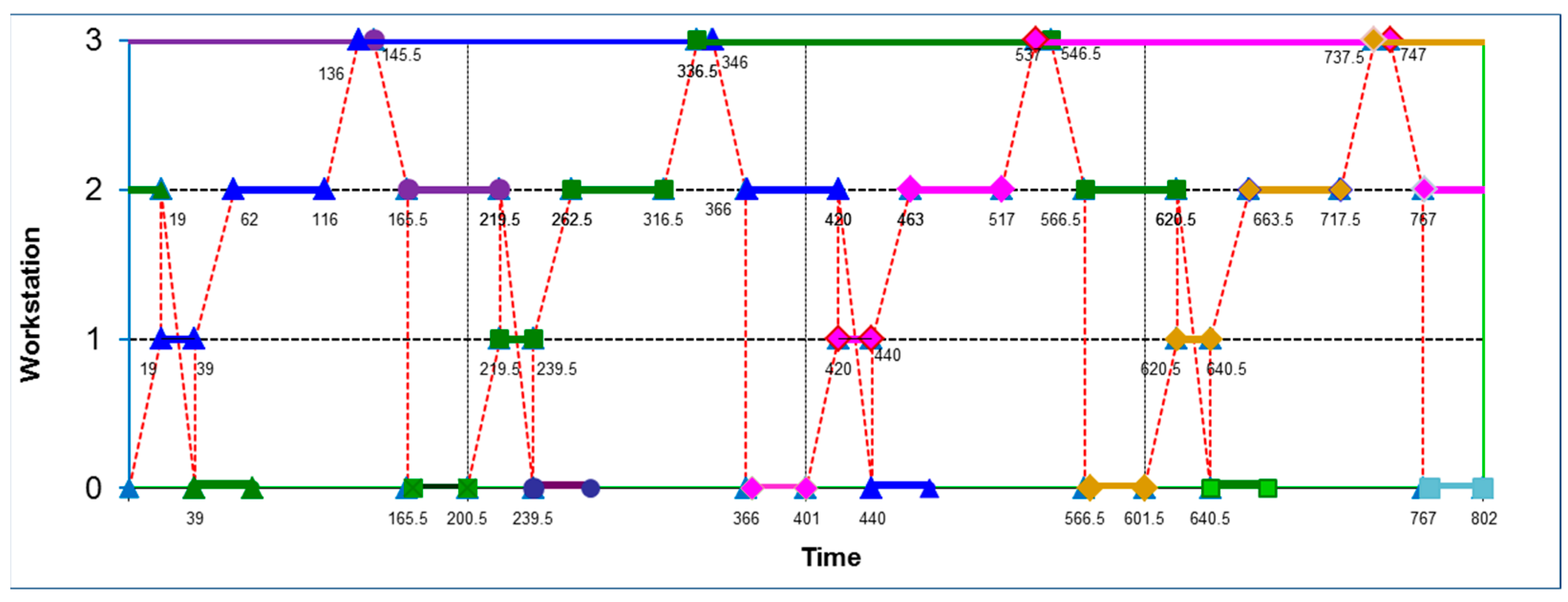
The Gantt chart of this 2-cyclic schedule is presented in Figure 5.

The Gantt chart in Figure 5 has the same notations as Figure 2. The main difference between the two diagrams is that Figure 5 shows the optimal 2-cyclic schedule of the robot. In this notation, the corresponding periodic route of the loaded robot is as follows:

R = (O_[1], O_[2], …, O_[10]) = (O₀, O₄, O₁, O₃, O₂, O₀, O₄, O₁, O₂, O₃).

As seen previously in Figure 2, the robot’s movement is shown with a red dotted line. The numbers in the chart indicate the time the robot arrives at and leaves the corresponding workstations. The processing life of microplates is indicated by horizontal lines highlighted with small triangles, squares, and diamonds, respectively. The optimal two-cyclic schedule shown in Figure 5 is (T₁, T₂) = (151, 250).

Complexity of the proposed PERT/CPM/PIM algorithm. In concluding this section, we note that the worst-case complexity of the parametric PERT/CPM algorithm in Section 4 is the same as the complexity of the corresponding critical path-finding algorithm in [21], that is, O(m³), while the complexity of the prohibited interval method is O(m³log m) [15]. Therefore, the complexity of the combined PERT/CPM/PIM algorithm, in the worst case, is O(m³log m).

Discussion. The main practical purpose of this work is twofold. First, we propose an algorithm that efficiently—in polynomial time—generates a set of optimal schedules with cycle times (T₁, T₂) = (191 + x, 210 − x), where x ∈ [0, 9.5], which includes, as particular cases, the optimal solutions obtained by methods [11,12,13,14]. Indeed, if x = 9.5, we obtain the one-cyclic schedule T = T₁ = T₂ = 200.5 found in [14]; if we set x = 0, then we obtain a 2-cyclic schedule with T₁ = 191 and T₂ = 210, the same as in [11]. Note that the 2-cyclic optimal schedule defined by times (T₁, T₂) = (151, 250) and the corresponding robot route R presented above have not been discovered by the algorithms [11,12,13,14].

Another important feature of the proposed method is that it significantly generalizes existing MIP and Petri net methods in the sense that it generates robust optimal two-cyclic schedules. Indeed, recall that a schedule is said to be robust if its cycle time T is insensitive to unexpected disturbances and/or can be easily corrected by a predetermined control policy. Let the resulting 2-cyclic schedule with times (T₁, T₂) = (191 + x, 210 − x) be fixed for some x ∈ (0, 9.5). Assume that due to unforeseen variations in the processing times of operations, a certain microplate, instead of the planned cycle time T₁, will be delayed by some fixed deviation δ, that is, it will have a cycle time T₁ + δ. The controller will then select the next scheduled microplate to start δ time units earlier, i.e., the next cycle time will be T₂ − δ. This simple control strategy ensures that the average cycle time T_avr remains stable: T_avr = (T₁ + δ + T₂ − δ)/2 = (T₁ + T₂)/2, that is, the resulting schedule is optimal and robust.

5. Conclusions

The problem considered in this study is to find an optimal robust cyclic schedule of robot movements that ensures maximum performance of the HTS system for biochemical analysis. To address this problem, we propose a new efficient PERT/CPM project management method, which works in combination with a modified prohibited intervals algorithm. To demonstrate the validity and practical utility of this method, we focus on the theoretical and numerical analysis of a real HTS process for enzymatic assay. The main result obtained is that the new combined PERT/CPM method is strongly polynomial, in contrast to existing mixed integer programming methods. Another advantage of the new method is that it is able to simultaneously generate a whole set of different optimal solutions, which can be used in practice for controlling unexpected fluctuations of input data. A characteristic feature of these results is that they have theoretical significance and at the same time have a strong applied focus.

While the present work focuses on HTS scheduling specifically for enzyme assays consisting of six workstations, the proposed mathematical model and project management techniques can be naturally extended to address and solve a variety of screening scheduling problems with a larger number of devices and more general formulations such as multi-degree cyclic scheduling, re-scheduling for unexpected disruptions, and the use of multiple robots to transport microplates. Since a wide variety of biochemical libraries are available today, each containing a huge number of compounds, it is essential to collect big data, compare results from different screens, schedule screening processes, and optimize them in an automated HTS system. These challenging problems can be addressed in future research by exploring new powerful and practice-oriented techniques from data science and artificial intelligence.

References

1. Aramaki, M.; Enjohji, K.; Yoshimura, M.; Sakawa, M.; Kato, K. HTS (high throughput screening) system scheduling through genetic algorithms. In Knowledge-Based Intelligent Information Engineering Systems & Allied Technologies, KES 2001; ISO Press: Osaka, Japan, 2001; pp. 1345–1349. [Google Scholar]
2. Blay, V.; Tolani, B.; Ho, S.P.; Arkin, M.R. High-throughput screening: Today’s biochemical and cell-based approaches. Drug Discov. Today 2020, 25, 1807–1821. [Google Scholar] [CrossRef] [PubMed]
3. Brunsch, T.; Raisch, J.; Hardouin, L. Modeling and control of high throughput screening systems. Control Eng. Pract. 2012, 20, 14–23. [Google Scholar] [CrossRef]
4. Murray, C.; Anderson, C. Scheduling software for high-throughput screening. Lab. Robot. Autom. 1996, 8, 295–305. [Google Scholar] [CrossRef]
5. Pinedo, M.L. Scheduling; Springer: New York, NY, USA, 2012. [Google Scholar]
6. Werner, F. (Ed.) Scheduling: Algorithms and Applications. Algorithms 2023, 16, 268. [Google Scholar] [CrossRef]
7. Werner, F.; Burtseva, L.; Sotskov, Y. Exact and Heuristic Scheduling; MDPI-Multidisciplinary Digital Publishing Institute: Basel, Switzerland, 2020. [Google Scholar]
8. Macarron, R. Critical review of the role of HTS in drug discovery. Drug Discov. Today 2006, 11, 277–279. [Google Scholar] [CrossRef]
9. Macarrón, R.; Hertzberg, R.P. Design and implementation of high throughput screening assays. Mol. Biotechnol. 2011, 47, 270–285. [Google Scholar] [CrossRef] [PubMed]
10. Major, J. Challenges and opportunities in high throughput screening: Implications for new technologies. J. Biomol. Screen. 1998, 3, 13–17. [Google Scholar] [CrossRef]
11. Oke, A.; Sahin, D.; Chen, X.; Shang, Y. High throughput screening for drug discovery and virus detection. Comb. Chem. High Throughput Screen. 2022, 25, 1518–1533. [Google Scholar]
12. Wu, N.Q.; Qiao, Y.; Li, Z.W. Efficient approach to scheduling of high throughput screening systems: A case study. In Proceedings of the IEEE 18th International Conference on Automation Science and Engineering (CASE), Mexico City, Mexico, 20–24 August 2022. [Google Scholar]
13. Oke, A.; Hardouin, L.; Chen, X.; Shang, Y. Scheduling and control of high throughput screening systems with uncertainties and disturbances. Prod. Manuf. Res. 2022, 10, 450–469. [Google Scholar] [CrossRef]
14. Wu, N.; Qiao, Y.; Li, Z.; Al-Ahmari, A.M.; El-Tamimi, A.A.; Kaid, H. A Novel control-theory-based approach to scheduling of high-throughput screening system for enzymatic assay. IEEE Trans. Syst. Man Cybern. Syst. 2022, 52, 7667–7678. [Google Scholar] [CrossRef]
15. Levner, E.; Kats, V.; Levit, V. An improved algorithm for cyclic flowshop scheduling in a robotic cell. Eur. J. Oper. Res. 1997, 97, 500–508. [Google Scholar] [CrossRef]
16. Brunsch, T. Modeling and Control of Complex Systems in a Dioid Framework. Ph.D. Thesis, Technische Universität, Berlin, Germany, 2013. Available online: https://depositonce.tu-berlin.de/bitstream/11303/4264/2/brunsch_thomas.pd (accessed on 27 March 2023).
17. Bagshaw, K.B. PERT and CPM in project management with practical examples. Am. J. Oper. Res. 2021, 11, 215–226. [Google Scholar] [CrossRef]
18. Vanhoucke, M.; Vanhoucke, M. The PERT/CPM Technique. In Project Management with Dynamic Scheduling: Baseline Scheduling, Risk Analysis and Project Control; Springer: Berlin/Heidelberg, Germany, 2013; pp. 11–35. [Google Scholar]
19. Lin, S.P.; Huang, D. Project Management under Internet Era; Springer: Berlin/Heidelberg, Germany, 2020. [Google Scholar]
20. Che, A.; Yan, P.; Yang, N.; Chu, C. Optimal cyclic scheduling of a hoist and multi-type parts with fixed processing times. Int. J. Prod. Res. 2010, 48, 1225–1243. [Google Scholar] [CrossRef]
21. Levner, E.; Kats, V. A parametric critical path problem and an application for cyclic scheduling. Discret. Appl. Math. 1998, 87, 149–158. [Google Scholar] [CrossRef]
22. Pang, X.; Xue, H.; Tseng, M.-L.; Lim, M.K.; Liu, K. Hybrid Flow Shop Scheduling Problems Using Improved Fireworks Algorithm for Permutation. Appl. Sci. 2020, 10, 1174. [Google Scholar] [CrossRef]
23. Janzen, W.P.; Bernasconi, P. (Eds.) High throughput screening: Methods and protocols. In Methods in Molecular Biology; Humana Press: Totowa, NJ, USA, 2009; Volume 565. [Google Scholar]
24. Mayer, E.; Raisch, J. Time-optimal scheduling for high throughput screening processes using cyclic discrete event models. Math. Comput. Simul. 2004, 66, 181–191. [Google Scholar] [CrossRef]
25. Mayr, L.M.; Fuerst, P. The future of high-throughput screening. SLAS Discov. 2008, 13, 443–448. [Google Scholar] [CrossRef]
26. Mayer, E.; Raisch, J. Modeling and optimization for high throughput-screening systems. Proc. IFAC 2004, 37, 469–474. [Google Scholar] [CrossRef]
27. Mayer, E.; Haus, U.-U.; Raisch, J.; Weismantel, R. Throughput optimal sequences for cyclically operated plants. Discrete Event Dyn. Syst. 2008, 18, 355–383. [Google Scholar] [CrossRef]
28. Suprunenko, D.A.; Aizenshtat, V.S.; Metel’sky, A.S. A multistage technological process. Dokl. Acad. Nauk BSSR 1962, 6, 522–541. (In Russian) [Google Scholar]
29. Aizenshtat, V.S. Multi-operator cyclic processes. Dokl. Byeloruss. Acad. Sci. 1963, 7, 224–227. (In Russian) [Google Scholar]
30. Tanaev, V.S. A scheduling problem for a flowshop line with a single operator. Eng. Phys. J. 1964, 7, 111–114. (In Russian) [Google Scholar]
Figure 1. HTS process flow diagram for an enzymatic assay.
Algorithms 17 00127 g001
Figure 2. The Gantt chart for a 1-cyclic schedule. R = (O0, O4, O1, O2, O3), T = 200.5.
Algorithms 17 00127 g002
Figure 3. Schematic diagram of the PERT/CPM/PIM algorithm.
Algorithms 17 00127 g003
Figure 4. PERT/CPM graph GP for the selected instance of problem Q.
Algorithms 17 00127 g004
Figure 5. The Gantt chart for the optimal two-cyclic schedule (T1, T2) = (151, 250), Tavr = 200.5.
Algorithms 17 00127 g005
Disclaimer/Publisher’s Note: The statements, opinions and data contained in all publications are solely those of the individual author(s) and contributor(s) and not of MDPI and/or the editor(s). MDPI and/or the editor(s) disclaim responsibility for any injury to people or property resulting from any ideas, methods, instructions or products referred to in the content.