1. Introduction
Numerical analysis is the area of mathematics that deals with computational techniques for studying and finding solutions to math problems. It is an offshoot of computer science and mathematics that develops, analyzes, and generates algorithms for numerically solving mathematical problems. Numerical methods are typically centered on the implementation of numerical algorithms. The goal of these numerical methods is to provide systematic procedures for numerically solving mathematical problems. The ordinary differential equation (ODE) is a mathematical equation that is used in natural physical processes, chemistry, engineering, and other sciences. Ordinary differential equations are notoriously difficult to approximate analytically, so the numerical treatment is crucial because it offers a powerful alternate solution method for resolving the differential equation.
We frequently use initial value problems (IVPs), such that
where
is the independent variable, which might also indicate time in physical problems, and
is the solution. Furthermore, because
can be a vector-valued function with N-dimensions, the domain and range of
and the solution
are given by
Furthermore, Equation (1), in which
is a function both of
and
, is known as a “non-autonomous” equation. However, by simply adding an extra variable, which is always equal to
, it can be easily rewritten in an equivalent “autonomous” form below, in which
is a function of
only:
There are numerous well-known numerical methods that can be used to solve the IVP in Equation (1). One category of these is third-order methods, like Ralston’s third-order Runge–Kutta method (Ralston’s scheme) [
1], the third-order Runge–Kutta method (RK3 scheme) [
2], the third-order Runge–Kutta method based on the arithmetic mean (ARK3 scheme) [
3], the third-order Heun’s method (Heun’s scheme) [
4], and several other methods. These numerical methods have been constructed to solve Equations (1) and (2) using different techniques such as the Taylor series expansion technique, homotopy analysis technique, quadrature formulas technique, and Adomian decomposition technique; for more details, see [
5,
6,
7].
In this study, we construct a new numerical method based on a variation of the standard formulation of the Runge–Kutta method using Taylor series expansion. The rest of this paper is divided into the following sections. In
Section 2, we recall some definitions and auxiliary results that we will use in our work. The derivation of the new method is described in
Section 3.
Section 4 provides details on the local truncation error.
Section 5 discusses the stability analysis of the suggested technique. The consistency of the new method and its convergence are detailed in
Section 6. Several numerical models are shown in
Section 7 to show the efficiency of this method and compare it with other relevant methods. Finally,
Section 8 offers the discussion and the conclusions.
2. Preliminaries
Theorem 1 ([
8])
. (Existence and Uniqueness Theorem). Let
and
be continuous functions of
and
at all points
in some neighborhood of the initial point
. Then, there is a unique function
defined on some interval
satisfying
Definition 1 ([
9])
. A Taylor sum or Taylor series is a mathematical function representation in the form of a series consisting of terms calculated using the values of the function’s derivation at a specific point and given by Definition 2 ([
10])
. Let be an open interval and be a -times differentiable function at . The Taylor polynomial of degree n at a point of is the polynomial Definition 3 ([
11])
. The difference between the numerical solution and the exact solution is called the local truncation error (L.T.E.) for a one-step method with step size is given by Definition 4 ([
12])
. The numerical method is said to be stable if there exists for each differential equation such that changing the initial values by a fixed amount produces a bounded change in the numerical solution for all Definition 5 ([
13])
. A numerical method is said to be consistent when all step sizes , as it will converge to the differential equation. In other words, we say the method is consistent if and only if 3. Construction of the New Scheme
In order to construct new single-step methods to solve the IVP Equation (1), we rely on a variant of the standard form of the Runge–Kutta method given by
where
and
and
By using the Taylor series expansion of any arbitrary function
for the non-autonomous Equation (1), we have
and in the autonomous case Equation (2),
becomes
We now start with the numerical method by using the family of explicit Runge–Kutta methods listed below to solve the mentioned problem in (2).
with
where
and
. We must first calculate the unknowns
,
and
. Using Taylor series expansion around
, we obtain
By expanding
,
, and
in Equations (11)–(13), we have
Substituting Equation (14) into Equation (9) yields
The Taylor series expansion of an exact solution
is given by
The following system of equations is obtained by expressing
and
in the Taylor expansion, ignoring terms with powers of
higher than 3, and then substituting them into formula (15) and comparing them to Equation (16):
This is a system with an infinite number of solutions comprising four equations and five unknowns. Assuming that
, we obtain the optimal solution listed below:
Additionally, from Equation (6), we obtain and .
Thus, substituting the above results in Equations (9) and (10), we present the new method, and we call it the variation Runge–Kutta method of order three (VRK3), given as follows:
with
4. Accuracy of the New Scheme
Here, the local truncation error of the proposed scheme is investigated as follows.
The set of Equation (18), when expanded using Taylor expansion, yields
Now, substituting Equations (19)–(21) into Equation (17) yields
Hence, from Definition 3, we have
As per Equation (22), our proposed method (VRK3) is of third order, with an of fourth order.
5. Stability Analysis of New Scheme
To test the absolute stability of the presented scheme (VRK3), we use the set of Equations (18) to derive the following:
By substituting Equations (23)–(25) into (17) and allowing
, we obtain
Then, from Equation (26), the stability polynomial is
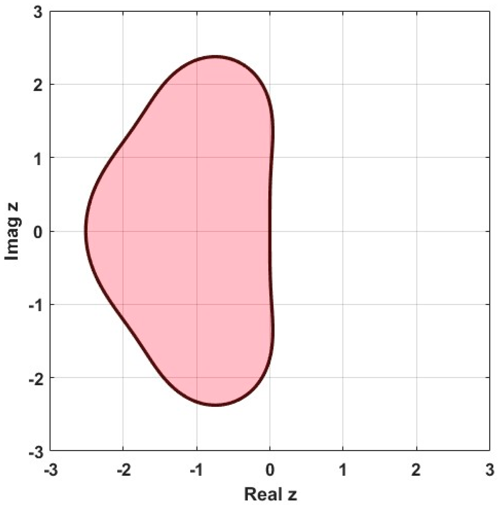
Utilizing the MATLAB program,
Figure 1 below graphically illustrates the absolute stability region of the Formula (27):
6. Consistency of the New Scheme
To explain the consistency property of the newly proposed scheme, we adopt Definition 5. Therefore, by substituting Equation (22) into Equation (8), we obtain
According to Lambert [
13], a numerical method is consistent if the order is bigger than one. Therefore, our new method is consistent since it is of order three.
Lambert also defines a numerical method as convergent if it is consistent and stable. Following from Equations (27) and (28), this method is consistent and stable. We conclude that the new method (VRK3) is convergent because it satisfies the consistency and stability properties.
7. Numerical Examples
In this section, we introduce two models of IVPs with varying step sizes
to compare the efficiency and the accuracy of the proposed new method (VRK3 scheme) with other third-order methods, like Ralston’s scheme, RK3 scheme, ARK3 scheme, and Heun’s scheme. Here, all calculations and figures are performed using MATLAB (R2022a) software. The numerical results are presented in
Table 1,
Table 2,
Table 3,
Table 4,
Table 5,
Table 6,
Table 7 and
Table 8, and the error analysis is illustrated in
Figure 2,
Figure 3,
Figure 4,
Figure 5,
Figure 6 and
Figure 7.
7.1. Problem 1 [14]
Take into consideration the first order IVP
,
, with the exact solution
,
.
Table 1,
Table 2 and
Table 3 show the results that were obtained. The graphs of absolute errors are shown in
Figure 2,
Figure 3 and
Figure 4. The comparison of CPU time between the VRK3 scheme and other relevant third-order schemes is shown in
Table 7.
Table 1.
Comparison of the absolute errors among third-order schemes in Problem 1, for .
Table 1.
Comparison of the absolute errors among third-order schemes in Problem 1, for .
| Ralston’s Scheme | RK3 Scheme | ARK3 Scheme | Heun’s Scheme | VRK3 Scheme |
|---|
| zero | zero | zero | zero | zero | zero |
| 0.1 | 6.2076 × 10⁻⁶ | 6.2076 × 10⁻⁶ | 8.9854 × 10⁻⁶ | 3.4299 × 10⁻⁶ | 6.5207 × 10⁻⁷ |
| 0.2 | 1.2845 × 10⁻⁵ | 1.2845 × 10⁻⁵ | 1.8692 × 10⁻⁵ | 6.9968 × 10⁻⁶ | 1.1492 × 10⁻⁶ |
| 0.3 | 1.9932 × 10⁻⁵ | 1.9932 × 10⁻⁵ | 2.9173 × 10⁻⁵ | 1.0692 × 10⁻⁵ | 1.4515 × 10⁻⁶ |
| 0.4 | 2.7492 × 10⁻⁵ | 2.7492 × 10⁻⁵ | 4.0482 × 10⁻⁵ | 1.4502 × 10⁻⁵ | 1.5125 × 10⁻⁶ |
| 0.5 | 3.5546 × 10⁻⁵ | 3.5546 × 10⁻⁵ | 5.2680 × 10⁻⁵ | 1.8412 × 10⁻⁵ | 1.2781 × 10⁻⁶ |
| 0.6 | 4.4113 × 10⁻⁵ | 4.4113 × 10⁻⁵ | 6.5826 × 10⁻⁵ | 2.2399 × 10⁻⁵ | 6.8563 × 10⁻⁷ |
| 0.7 | 5.3212 × 10⁻⁵ | 5.3212 × 10⁻⁵ | 7.9987 × 10⁻⁵ | 2.6437 × 10⁻⁵ | 3.3777 × 10⁻⁷ |
| 0.8 | 6.2861 × 10⁻⁵ | 6.2861 × 10⁻⁵ | 9.5229 × 10⁻⁵ | 3.0492 × 10⁻⁵ | 1.8762 × 10⁻⁶ |
| 0.9 | 7.3074 × 10⁻⁵ | 7.3074 × 10⁻⁵ | 1.1162 × 10⁻⁴ | 3.4524 × 10⁻⁵ | 4.0265 × 10⁻⁶ |
| 1 | 8.3864 × 10⁻⁵ | 8.3864 × 10⁻⁵ | 1.2925 × 10⁻⁴ | 3.8482 × 10⁻⁵ | 6.9006 × 10⁻⁶ |
Table 2.
Comparison of the absolute errors among third-order schemes in Problem 1, for .
Table 2.
Comparison of the absolute errors among third-order schemes in Problem 1, for .
| Ralston’s Scheme | RK3 Scheme | ARK3 Scheme | Heun’s Scheme | VRK3 Scheme |
|---|
| zero | zero | zero | zero | zero | zero |
| 0.1 | 7.9184 × 10⁻⁷ | 7.9184 × 10⁻⁷ | 1.1480 × 10⁻⁶ | 4.3572 × 10⁻⁷ | 7.9594 × 10⁻⁸ |
| 0.2 | 1.6379 × 10⁻⁶ | 1.6379 × 10⁻⁶ | 2.3876 × 10⁻⁶ | 8.8818 × 10⁻⁷ | 1.3848 × 10⁻⁷ |
| 0.3 | 2.5408 × 10⁻⁶ | 2.5408 × 10⁻⁶ | 3.7254 × 10⁻⁶ | 1.3561 × 10⁻⁶ | 1.7141 × 10⁻⁷ |
| 0.4 | 3.5031 × 10⁻⁶ | 3.5031 × 10⁻⁶ | 5.1684 × 10⁻⁶ | 1.8377 × 10⁻⁶ | 1.7229 × 10⁻⁷ |
| 0.5 | 4.5273 × 10⁻⁶ | 4.5273 × 10⁻⁶ | 6.7240 × 10⁻⁶ | 2.3307 × 10⁻⁶ | 1.3400 × 10⁻⁷ |
| 0.6 | 5.6159 × 10⁻⁶ | 5.6159 × 10⁻⁶ | 8.3997 × 10⁻⁶ | 2.8321 × 10⁻⁶ | 4.8292 × 10⁻⁸ |
| 0.7 | 6.7710 × 10⁻⁶ | 6.7710 × 10⁻⁶ | 1.0204 × 10⁻⁵ | 3.3383 × 10⁻⁶ | 9.4375 × 10⁻⁸ |
| 0.8 | 7.9947 × 10⁻⁶ | 7.9947 × 10⁻⁶ | 1.2144 × 10⁻⁵ | 3.8448 × 10⁻⁶ | 3.0504 × 10⁻⁷ |
| 0.9 | 9.2884 × 10⁻⁶ | 9.2884 × 10⁻⁶ | 1.4231 × 10⁻⁵ | 4.3460 × 10⁻⁶ | 5.9642 × 10⁻⁷ |
| 1 | 1.0653 × 10⁻⁵ | 1.0653 × 10⁻⁵ | 1.6472 × 10⁻⁵ | 4.8351 × 10⁻⁶ | 9.8318 × 10⁻⁷ |
Table 3.
Comparison of the absolute errors among third-order schemes in Problem 1, for .
Table 3.
Comparison of the absolute errors among third-order schemes in Problem 1, for .
| Ralston’s Scheme | RK3 Scheme | ARK3 Scheme | Heun’s Scheme | VRK3 Scheme |
|---|
| zero | zero | zero | zero | zero | zero |
| 0.1 | 9.9973 × 10⁻⁸ | 9.9973 × 10⁻⁸ | 1.4505 × 10⁻⁷ | 5.4894 × 10⁻⁸ | 9.8153 × 10⁻⁹ |
| 0.2 | 2.0675 × 10⁻⁷ | 2.0675 × 10⁻⁷ | 3.0165 × 10⁻⁷ | 1.1185 × 10⁻⁷ | 1.6954 × 10⁻⁸ |
| 0.3 | 3.2066 × 10⁻⁷ | 3.2066 × 10⁻⁷ | 4.7062 × 10⁻⁷ | 1.7070 × 10⁻⁷ | 2.0745 × 10⁻⁸ |
| 0.4 | 4.4202 × 10⁻⁷ | 4.4202 × 10⁻⁷ | 6.5283 × 10⁻⁷ | 2.3121 × 10⁻⁷ | 2.0405 × 10⁻⁸ |
| 0.5 | 5.7114 × 10⁻⁷ | 5.7114 × 10⁻⁷ | 8.4920 × 10⁻⁷ | 2.9308 × 10⁻⁷ | 1.5023 × 10⁻⁸ |
| 0.6 | 7.0830 × 10⁻⁷ | 7.0830 × 10⁻⁷ | 1.0607 × 10⁻⁶ | 3.5592 × 10⁻⁷ | 3.5422 × 10⁻⁹ |
| 0.7 | 8.5378 × 10⁻⁷ | 8.5378 × 10⁻⁷ | 1.2883 × 10⁻⁶ | 4.1926 × 10⁻⁷ | 1.5261 × 10⁻⁸ |
| 0.8 | 1.0078 × 10⁻⁶ | 1.0078 × 10⁻⁶ | 1.5331 × 10⁻⁶ | 4.8250 × 10⁻⁷ | 4.2799 × 10⁻⁸ |
| 0.9 | 1.1705 × 10⁻⁶ | 1.1705 × 10⁻⁶ | 1.7962 × 10⁻⁶ | 5.4492 × 10⁻⁷ | 8.0702 × 10⁻⁸ |
| 1 | 1.3422 × 10⁻⁶ | 1.3422 × 10⁻⁶ | 2.0787 × 10⁻⁶ | 6.0565 × 10⁻⁷ | 1.3084 × 10⁻⁷ |
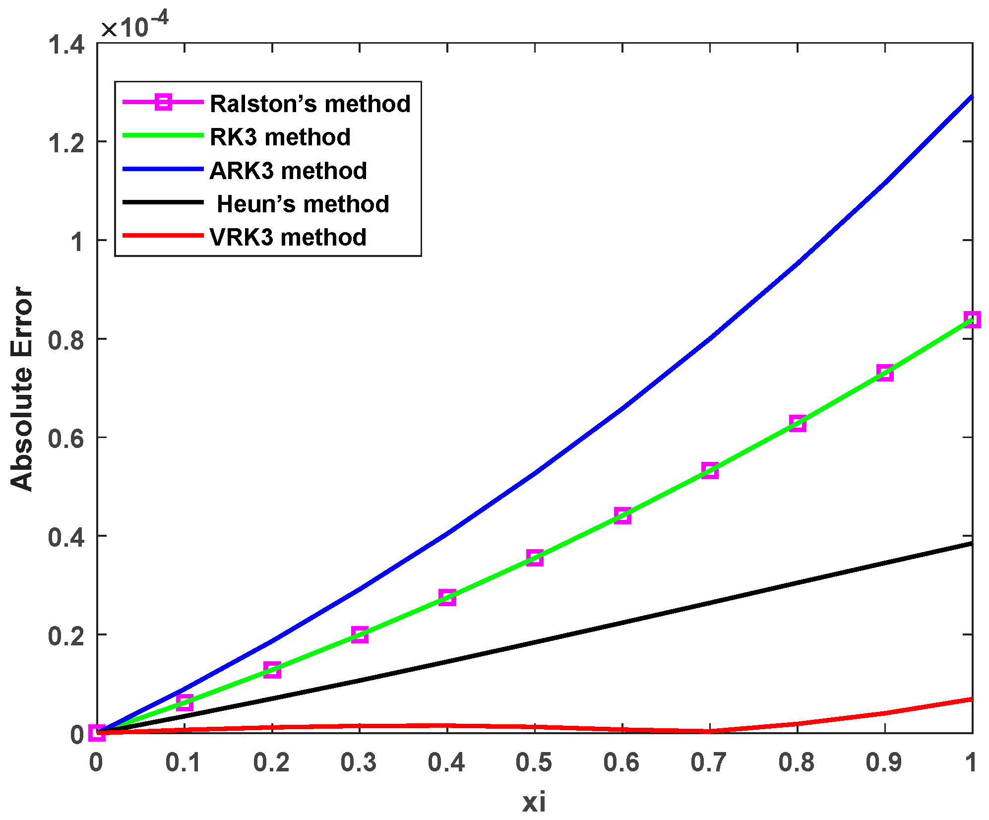
Figure 2.
The absolute errors for numerical results in
Table 1.
Figure 2.
The absolute errors for numerical results in
Table 1.
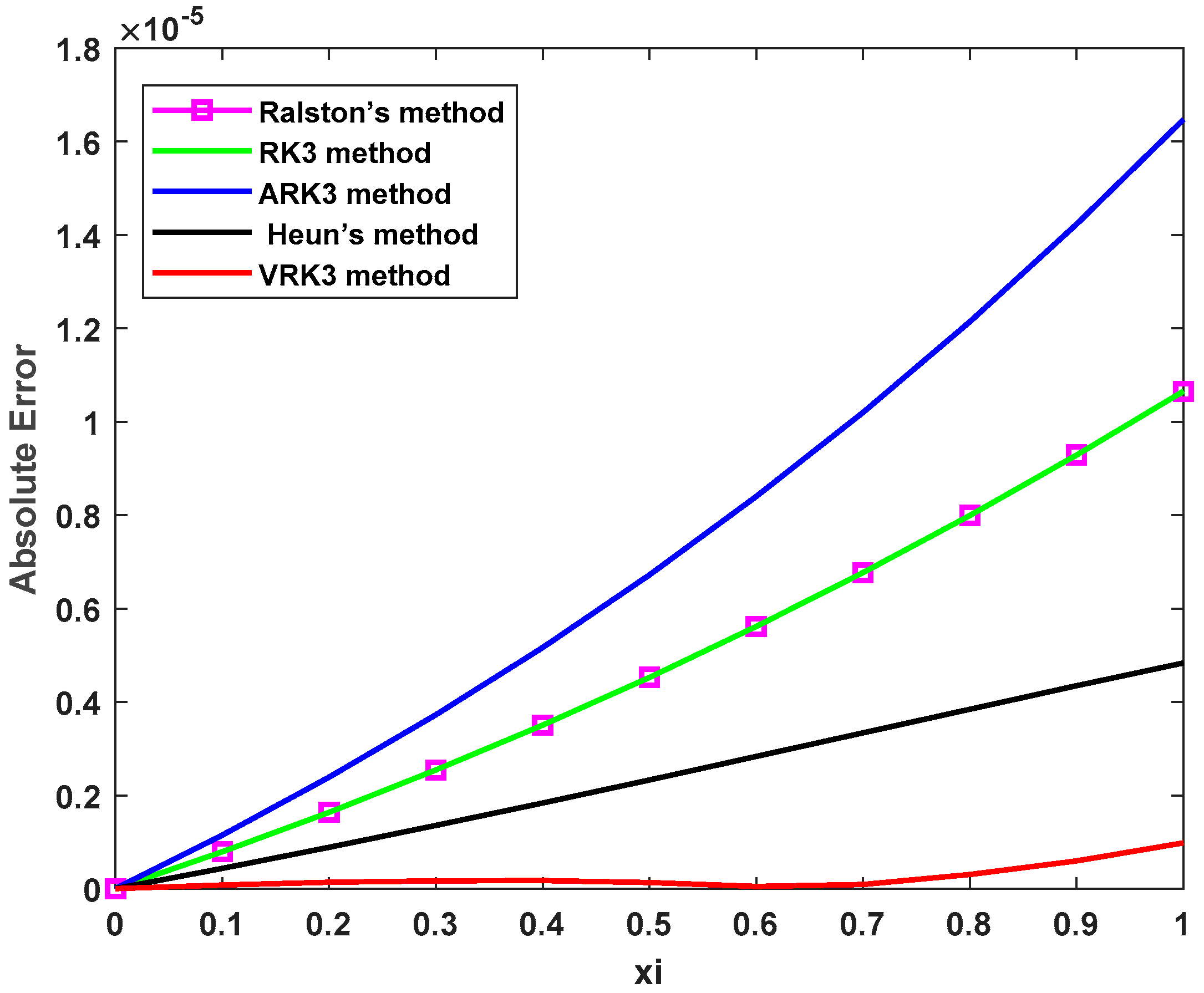
Figure 3.
The absolute errors for numerical results in
Table 2.
Figure 3.
The absolute errors for numerical results in
Table 2.
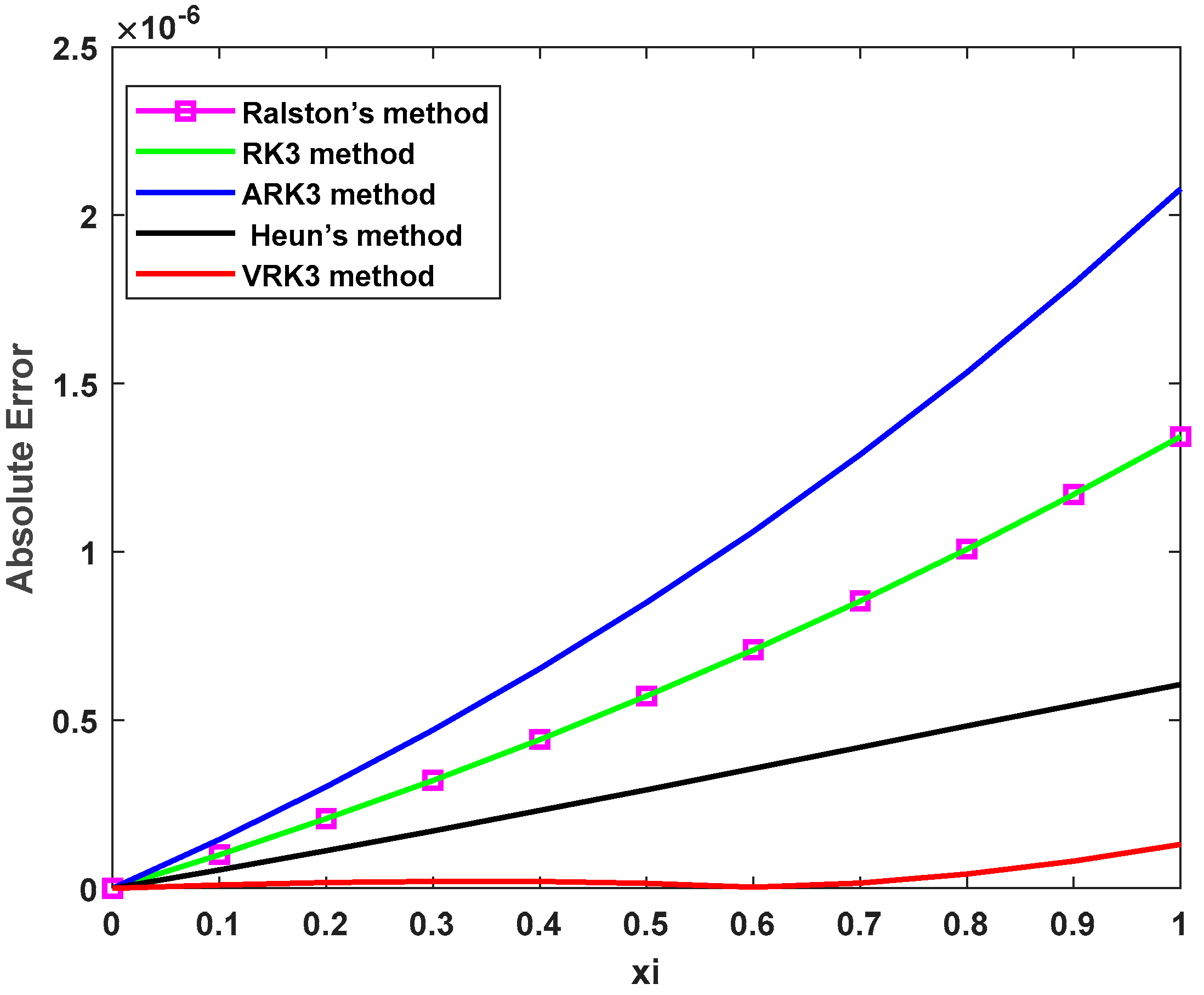
Figure 4.
The absolute errors for numerical results in
Table 3.
Figure 4.
The absolute errors for numerical results in
Table 3.
7.2. Problem 2 (Mixture Model)
We consider here the IVP proposed in [
15], which was a model of a storage tank in an oil refinery that holds
gal of gasoline with
lb of an additive mixed within it. To prepare for winter weather,
gal/min of gasoline that contains
lb of additive per gallon is pumped into the storage tank. The well-mixed solution is pumped out at a rate of
gal/min. Let
be the amount of additive (in pounds) in the tank at time
. When
, we know that
. The mixture process is modeled by the IVP,
, and the analytic solution,
},
.
Table 4,
Table 5 and
Table 6 show the absolute errors among third-order methods and the VRK3 scheme, with different step sizes of
,
, and
.
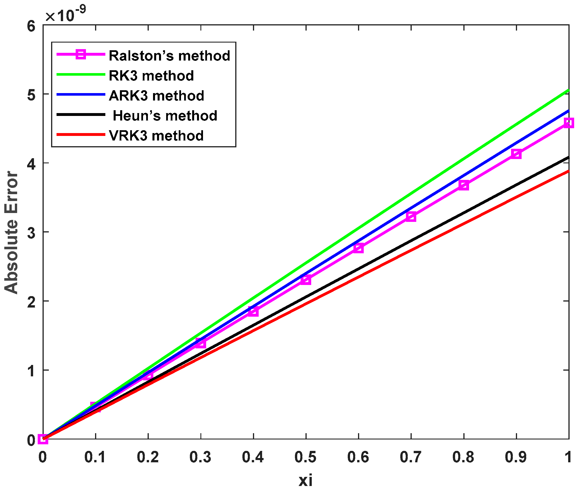
Figure 5,
Figure 6 and
Figure 7 depict the graphical analysis used to support the numerical results in
Table 4,
Table 5 and
Table 6. A comparison of CPU time between the new method and other third-order schemes is shown in
Table 8.
Table 4.
Comparison of the absolute errors among third-order schemes in Problem 2, for .
Table 4.
Comparison of the absolute errors among third-order schemes in Problem 2, for .
| Ralston’s Scheme | RK3 Scheme | ARK3 Scheme | Heun’s Scheme | VRK3 Scheme |
|---|
| zero | zero | zero | zero | zero | zero |
| 0.1 | 3.7246 × 10⁻⁹ | 4.1133 × 10⁻⁹ | 3.8694 × 10⁻⁹ | 3.3207 × 10⁻⁹ | 3.1607 × 10⁻⁹ |
| 0.2 | 7.4366 × 10⁻⁹ | 8.2127 × 10⁻⁹ | 7.7257 × 10⁻⁹ | 6.6303 × 10⁻⁹ | 6.3109 × 10⁻⁹ |
| 0.3 | 1.1136 × 10⁻⁸ | 1.2298 × 10⁻⁸ | 1.1568 × 10⁻⁸ | 9.9282 × 10⁻⁹ | 9.4499 × 10⁻⁹ |
| 0.4 | 1.4821 × 10⁻⁸ | 1.6367 × 10⁻⁸ | 1.5397 × 10⁻⁸ | 1.3214 × 10⁻⁸ | 1.2577 × 10⁻⁸ |
| 0.5 | 1.8494 × 10⁻⁸ | 2.0424 × 10⁻⁸ | 1.9213 × 10⁻⁸ | 1.6488 × 10⁻⁸ | 1.5694 × 10⁻⁸ |
| 0.6 | 2.2154 × 10⁻⁸ | 2.4466 × 10⁻⁸ | 2.3015 × 10⁻⁸ | 1.9752 × 10⁻⁸ | 1.8800 × 10⁻⁸ |
| 0.7 | 2.5801 × 10⁻⁸ | 2.8493 × 10⁻⁸ | 2.6804 × 10⁻⁸ | 2.3003 × 10⁻⁸ | 2.1895 × 10⁻⁸ |
| 0.8 | 2.9435 × 10⁻⁸ | 3.2507 × 10⁻⁸ | 3.0579 × 10⁻⁸ | 2.6243 × 10⁻⁸ | 2.4979 × 10⁻⁸ |
| 0.9 | 3.3057 × 10⁻⁸ | 3.6506 × 10⁻⁸ | 3.4342 × 10⁻⁸ | 2.9472 × 10⁻⁸ | 2.8053 × 10⁻⁸ |
| 1 | 3.6665 × 10⁻⁸ | 4.0491 × 10⁻⁸ | 3.8090 × 10⁻⁸ | 3.2689 × 10⁻⁸ | 3.1114 × 10⁻⁸ |
Table 5.
Comparison of the absolute errors among third-order schemes in Problem 2, for .
Table 5.
Comparison of the absolute errors among third-order schemes in Problem 2, for .
| Ralston’s Scheme | RK3 Scheme | ARK3 Scheme | Heun’s Scheme | VRK3 Scheme |
|---|
| zero | zero | zero | zero | zero | zero |
| 0.1 | 4.6501 × 10⁻¹⁰ | 5.1354 × 10⁻¹⁰ | 4.8308 × 10⁻¹⁰ | 4.1457 × 10⁻¹⁰ | 3.9459 × 10⁻¹⁰ |
| 0.2 | 9.2889 × 10⁻¹⁰ | 1.0258 × 10⁻⁹ | 9.6499 × 10⁻¹⁰ | 8.2821 × 10⁻¹⁰ | 7.8832 × 10⁻¹⁰ |
| 0.3 | 1.3910 × 10⁻⁹ | 1.5361 × 10⁻⁹ | 1.4451 × 10⁻⁹ | 1.2403 × 10⁻⁹ | 1.1805 × 10⁻⁹ |
| 0.4 | 1.8506 × 10⁻⁹ | 2.0437 × 10⁻⁹ | 1.9225 × 10⁻⁹ | 1.6499 × 10⁻⁹ | 1.5704 × 10⁻⁹ |
| 0.5 | 2.3096 × 10⁻⁹ | 2.5506 × 10⁻⁹ | 2.3994 × 10⁻⁹ | 2.0592 × 10⁻⁹ | 1.9600 × 10⁻⁹ |
| 0.6 | 2.7670 × 10⁻⁹ | 3.0556 × 10⁻⁹ | 2.8745 × 10⁻⁹ | 2.4671 × 10⁻⁹ | 2.3482 × 10⁻⁹ |
| 0.7 | 3.2222 × 10⁻⁹ | 3.5584 × 10⁻⁹ | 3.3474 × 10⁻⁹ | 2.8729 × 10⁻⁹ | 2.7345 × 10⁻⁹ |
| 0.8 | 3.6763 × 10⁻⁹ | 4.0598 × 10⁻⁹ | 3.8191 × 10⁻⁹ | 3.2778 × 10⁻⁹ | 3.1199 × 10⁻⁹ |
| 0.9 | 4.1288 × 10⁻⁹ | 4.5595 × 10⁻⁹ | 4.2892 × 10⁻⁹ | 3.6813 × 10⁻⁹ | 3.5040 × 10⁻⁹ |
| 1 | 4.5789 × 10⁻⁹ | 5.0566 × 10⁻⁹ | 4.7568 × 10⁻⁹ | 4.0826 × 10⁻⁹ | 3.8859 × 10⁻⁹ |
Table 6.
Comparison of the absolute errors among third-order schemes in Problem 2, for .
Table 6.
Comparison of the absolute errors among third-order schemes in Problem 2, for .
| Ralston’s Scheme | RK3 Scheme | ARK3 Scheme | Heun’s Scheme | VRK3 Scheme |
|---|
| zero | zero | zero | zero | zero | zero |
| 0.1 | 5.7938 × 10⁻¹¹ | 6.4006 × 10⁻¹¹ | 6.0197 × 10⁻¹¹ | 5.1628 × 10⁻¹¹ | 4.9127 × 10⁻¹¹ |
| 0.2 | 1.1617 × 10⁻¹⁰ | 1.2828 × 10⁻¹⁰ | 1.2069 × 10⁻¹⁰ | 1.0360 × 10⁻¹⁰ | 9.8595 × 10⁻¹¹ |
| 0.3 | 1.7408 × 10⁻¹⁰ | 1.9220 × 10⁻¹⁰ | 1.8083 × 10⁻¹⁰ | 1.5525 × 10⁻¹⁰ | 1.4776 × 10⁻¹⁰ |
| 0.4 | 2.3087 × 10⁻¹⁰ | 2.5497 × 10⁻¹⁰ | 2.3985 × 10⁻¹⁰ | 2.0580 × 10⁻¹⁰ | 1.9583 × 10⁻¹⁰ |
| 0.5 | 2.8851 × 10⁻¹⁰ | 3.1858 × 10⁻¹⁰ | 2.9971 × 10⁻¹⁰ | 2.5724 × 10⁻¹⁰ | 2.4477 × 10⁻¹⁰ |
| 0.6 | 3.4589 × 10⁻¹⁰ | 3.8193 × 10⁻¹⁰ | 3.5934 × 10⁻¹⁰ | 3.0846 × 10⁻¹⁰ | 2.9351 × 10⁻¹⁰ |
| 0.7 | 4.0254 × 10⁻¹⁰ | 4.4454 × 10⁻¹⁰ | 4.1820 × 10⁻¹⁰ | 3.5894 × 10⁻¹⁰ | 3.4157 × 10⁻¹⁰ |
| 0.8 | 4.5941 × 10⁻¹⁰ | 5.0736 × 10⁻¹⁰ | 4.7731 × 10⁻¹⁰ | 4.0967 × 10⁻¹⁰ | 3.8989 × 10⁻¹⁰ |
| 0.9 | 5.1622 × 10⁻¹⁰ | 5.7003 × 10⁻¹⁰ | 5.3629 × 10⁻¹⁰ | 4.6035 × 10⁻¹⁰ | 4.3809 × 10⁻¹⁰ |
| 1 | 5.7196 × 10⁻¹⁰ | 6.3162 × 10⁻¹⁰ | 5.9421 × 10⁻¹⁰ | 5.0994 × 10⁻¹⁰ | 4.8530 × 10⁻¹⁰ |
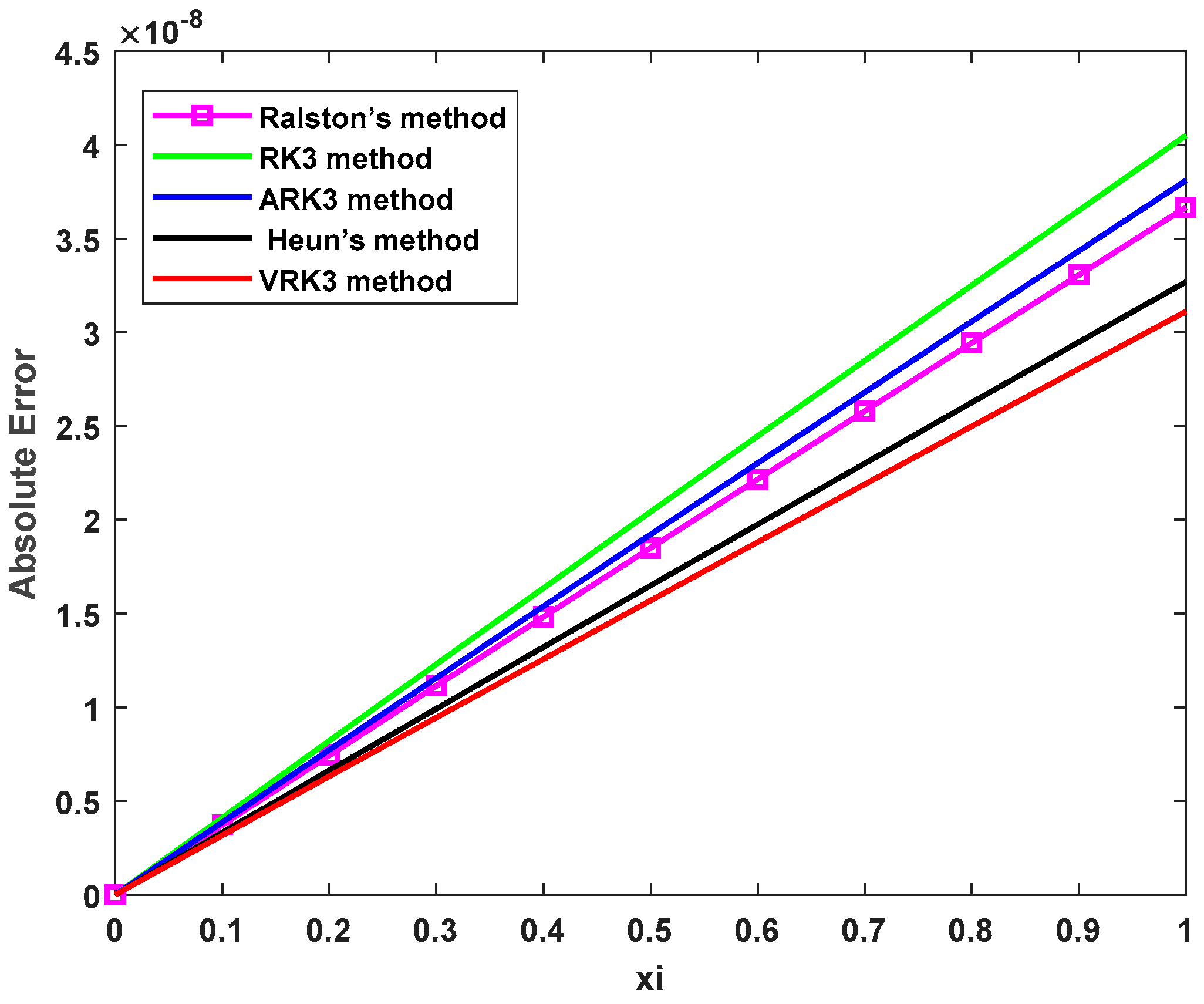
Figure 5.
The absolute errors for numerical results in
Table 4.
Figure 5.
The absolute errors for numerical results in
Table 4.
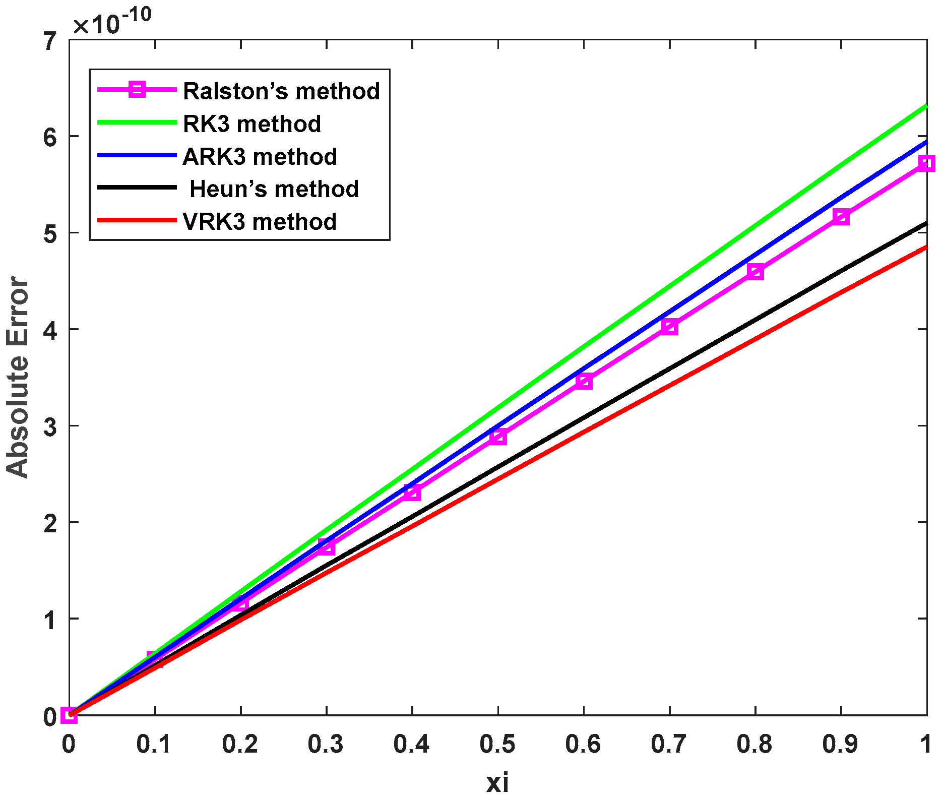
Figure 6.
The absolute errors for numerical results in
Table 5.
Figure 6.
The absolute errors for numerical results in
Table 5.
Figure 7.
The absolute errors for numerical results in
Table 6.
Figure 7.
The absolute errors for numerical results in
Table 6.
Table 7.
Comparisons of CPU time in Problem 1, for different step sizes h.
Table 7.
Comparisons of CPU time in Problem 1, for different step sizes h.
| Step Size | CPU Time |
|---|
| Ralston’s Scheme | RK3 Scheme | ARK3 Scheme | Heun’s Scheme | VRK3 Scheme |
|---|
| h = 0.1 | 0.003325 | 0.003508 | 0.004631 | 0.005653 | 0.001558 |
| h = 0.05 | 0.003407 | 0.004827 | 0.003017 | 0.005066 | 0.001027 |
| h = 0.025 | 0.003655 | 0.003144 | 0.005021 | 0.004364 | 0.001273 |
Table 8.
Comparisons of CPU time in Problem 2, for different step sizes h.
Table 8.
Comparisons of CPU time in Problem 2, for different step sizes h.
| Step Size | CPU Time |
|---|
| Ralston’s Scheme | RK3 Scheme | ARK3 Scheme | HEUN’S SCHEME | VRK3 Scheme |
|---|
| h = 0.1 | 0.004160 | 0.003116 | 0.004698 | 0.004627 | 0.001358 |
| h = 0.05 | 0.003328 | 0.004782 | 0.004879 | 0.003469 | 0.001003 |
| h = 0.025 | 0.003506 | 0.004392 | 0.003230 | 0.004234 | 0.001296 |
8. Discussion and Conclusions
In this study, we introduced an innovative third-order method designed for solving initial value problems (IVPs). Our approach is rooted in a novel adaptation of the standard formulation employed in Runge–Kutta methods, incorporating Taylor series expansion. To validate the effectiveness of this new method, we employed two distinct numerical models, effectively showcasing its fundamental capabilities. It is important to underscore that all our numerical findings, including the accompanying tables and figures, were calculated using MATLAB (R2022a) software on a dedicated computer system operating with Windows 11 Pro. The system uses an 11th Generation Intel(R) Core (TM) i7-11800H processor running at 2.30 GHz, backed by 16.0 GB of RAM (15.7 GB usable).
A comprehensive numerical assessment was conducted using
Table 1,
Table 2,
Table 3,
Table 4,
Table 5 and
Table 6, which present an intricate comparison of absolute errors across various step sizes, specifically
. Through the graphical representations found in
Figure 2,
Figure 3,
Figure 4,
Figure 5,
Figure 6 and
Figure 7, we were able to discern that our novel method, referred to as VRK3, consistently outperformed several benchmark techniques including Ralston’s scheme, RK3 scheme, ARK3 scheme, and Heun’s scheme. This superiority primarily stems from the reduced local truncation error of VRK3. Additionally, our investigation revealed a significant insight regarding the impact of step size on accuracy. As we decreased the step size, the error progressively approached zero, strongly indicating that precision increased with smaller step sizes. This observation reinforces the importance of carefully selecting step sizes to achieve higher levels of accuracy in numerical solutions. Turning our attention to computational efficiency,
Table 7 and
Table 8 provided valuable insights. The VRK3 scheme consistently demonstrated reduced CPU time compared to its counterparts, further validating its utility in practical applications. Furthermore,
Figure 1 depicts the stability region of our third-order VRK3 scheme, establishing its equivalence to similar methodologies. Importantly, we substantiated the convergence of our VRK3 scheme, as it satisfies both the consistency and stability criteria.
In conclusion, our newly proposed third-order method exhibits a commendable blend of efficiency and reliability. The method’s stability and high accuracy render it particularly robust for a wide range of applications. This research contributes to the field of numerical methods for IVPs by presenting an innovative approach that holds promise for improving computational accuracy and efficiency. Future research directions might explore the extension of this method to more complex problems or its integration into broader computational frameworks.
Author Contributions
Conceptualization, N.Y.A.-H., Z.J.K. and A.H.A.; formal analysis, N.Y.A.-H., Z.J.K. and A.H.A.; investigation, N.Y.A.-H., Z.J.K. and A.H.A.; methodology, N.Y.A.-H., Z.J.K. and A.H.A.; software, A.H.A.; supervision, N.Y.A.-H.; writing—original draft, N.Y.A.-H. and Z.J.K.; writing—review and editing, A.H.A. All authors have read and agreed to the published version of the manuscript.
Funding
The author received no direct funding for this work.
Institutional Review Board Statement
Not applicable.
Informed Consent Statement
Not applicable.
Data Availability Statement
Data are contained within the article.
Acknowledgments
The author would like to express gratitude to the anonymous referees for their valuable comments and suggestions.
Conflicts of Interest
The authors declare that they have no competing interests.
References
- Ralston, A. Runge-Kutta Methods with Minimum Error Bounds. Math. Comput. 1962, 16, 431–437. [Google Scholar] [CrossRef]
- Ralston, A.; Rabinowitz, P. A First Course in Numerical Analysis, 2nd ed.; McGraw-Hill: New York, NY, USA, 1978. [Google Scholar]
- Wazwaz, A.M. A Comparison of Modified Runge-Kutta Formulas Based on a Variety of Means. Int. J. Comput. Math. 1994, 50, 105–112. [Google Scholar] [CrossRef]
- Hatun, M.; Vatansever, F. Differential Equation Solver Simulator for Runge-Kutta Methods. Uludağ Univ. J. Fac. Eng. 2016, 21, 145–162. [Google Scholar]
- Burden, R.L.; Faires, J.D. Numerical Analysis, 9th ed.; Brooks/Cole Publishing Company: Pacific Grove, CA, USA, 2011. [Google Scholar]
- Ahmad, N.; Charan, S. A Comparative Study on Numerical Solution of Ordinary Differential Equation by Different Method with Initial Value Problem. Int. J. Recent. Sci. Res. 2017, 8, 21134–21139. [Google Scholar]
- Nhawu, G.; Mafuta, P.; Mushanyu, J. The Adomian Decomposition Method for Numerical Solution of First-Order Differential Equations. J. Math. Comput. Sci. 2016, 6, 307–314. [Google Scholar]
- Nagle, R.K.; Saff, E.B.; Snider, A.D. Fundamentals of Differential Equations, 9th ed.; Pearson: Boston, MA, USA, 2018. [Google Scholar]
- Wusu, A.S.; Akanbi, M.A.; Okunuga, S.A. A Three-stage Multiderivative Explicit Runge-Kutta Method. Am. J. Comput. Math. 2013, 3, 121–126. [Google Scholar]
- Ali, A.H.; Pales, Z.S. Taylor-type Expansions in Terms of Exponential Polynomials. Math. Inequalities Appl. 2022, 25, 1123–1141. [Google Scholar] [CrossRef]
- Kadum, Z.J.; Abdul-Hassan, N.Y. New Numerical Methods for Solving the Initial Value Problem Based on a Symmetrical Quadrature Integration Formula Using Hybrid Functions. Symmetry 2023, 15, 631. [Google Scholar] [CrossRef]
- Corless, R.M.; Kaya, C.Y.; Moir, R.H.C. Optimal Residuals and the Dahlquist Test Problem. Numer. Algorithms 2019, 81, 1253–1274. [Google Scholar] [CrossRef]
- Lambert, J.D. Computational Methods in Ordinary Differential Equations; John Wiley & Sons Inc.: New York, NY, USA, 1973. [Google Scholar]
- Ram, T.; Solangi, M.A.; Sanghah, A.A. A Hybrid Numerical Method with Greater Efficiency for Solving Initial Value Problems. Math. Theory Model. 2020, 10, 2224–5804. [Google Scholar]
- Omar, Z.; Adeyeye, O. Numerical Solution of First Order Initial Value Problems Using a Self-Starting Implicit Two-Step Obrechkoff-Type Block Method. J. Math. Stat. 2016, 12, 127–134. [Google Scholar] [CrossRef]
| Disclaimer/Publisher’s Note: The statements, opinions and data contained in all publications are solely those of the individual author(s) and contributor(s) and not of MDPI and/or the editor(s). MDPI and/or the editor(s) disclaim responsibility for any injury to people or property resulting from any ideas, methods, instructions or products referred to in the content. |
© 2024 by the authors. Licensee MDPI, Basel, Switzerland. This article is an open access article distributed under the terms and conditions of the Creative Commons Attribution (CC BY) license (https://creativecommons.org/licenses/by/4.0/).


