Modeling of Some Classes of Extended Oscillators: Simulations, Algorithms, Generating Chaos, and Open Problems

Abstract

In this article, we propose some extended oscillator models. Various experiments are performed. The models are studied using the Melnikov approach. We show some integral units for researching the behavior of these hypothetical oscillators. These will be implemented as add-on sections of a thoughtful main web-based application for researching computations. One of the main goals of the study is to share the difficulties that researchers (who are not necessarily professional mathematicians) encounter in using contemporary computer algebraic systems (CASs) for scientific research to examine in detail the dynamics of modifications of classical and newer models that are emerging in the literature (for the large values of the parameters of the models). The present article is a natural continuation of the research in the direction that has been indicated and discussed in our previous investigations. One possible application that the Melnikov function may find in the modeling of a radiating antenna diagram is also discussed. Some probability-based constructions are also presented. We hope that some of these notes will be reflected in upcoming registered rectifications of the CAS. The aim of studying the design realization (scheme, manufacture, output, etc.) of the explored differential models can be viewed as not yet being met.

1. Introduction

Multiple natural phenomena of the oscillatory kind that appear in a variety of disciplines, such as mechanics, quantum optics, acoustics, hydrodynamics, electronics, and engineering, have the possibility of ensuring the freedom of a potential well, and are portrayed by a general escape nonlinear oscillator model. Sanjuan [1] considers the equation of movement for the sinusoidal-driven escape oscillator, incorporating nonlinear damping conditions as a power series on the speed reads:

$$\ddot{x}+{\displaystyle \sum _{p=1}^n}\beta \dot{x}{\left|\dot{x}\right|}^{p-1}+x-x^2=Fsin\omega t,$$

(1)

where $\beta$ is the damping level, p is the damping exponent, and F and $\omega$ are the forcing amplitude and the frequency of the outer disturbance, respectively. Specifically, the following system is considered

$$\left\{\begin{array}{ccc}{\displaystyle \frac{dx}{dt}}\hfill & =& y\hfill \\ {\displaystyle \frac{dy}{dt}}\hfill & =& -x+x^2-\beta y{\left|y\right|}^{p-1}+Fsin\omega t,\hfill \end{array}\right.$$

(2)

where—for simplification—at most a lone damping term in proportion to the $p\mathrm{th}$ power of the speed is taken.

The critical forcing parameter $F_{cp}$, for which homoclinic entangles intersect, for a fixed frequency $\omega$, is a function of the damping exponent p and the damping factor $\beta$; this may be expressed as [1]:

$$F_{cp}=\beta \frac{sinh\left(\pi \omega \right)}{3\pi {\omega }^2}{\left(\frac{3}{2}\right)}^{p+1}B\left(\frac{p+2}{2},\frac{p+1}{2}\right)$$

where $B(m,n)$ is the Euler Beta function.

The nonlinear vessel trundling reply and nonlinearly damped general escape oscillator can be represented in the following way:

$$\left\{\begin{array}{ccc}{\displaystyle \frac{dx}{dt}}\hfill & =& y\hfill \\ {\displaystyle \frac{dy}{dt}}\hfill & =& -{\displaystyle \sum _{j=1}^m}{a}_j{x}^j+{\displaystyle \sum _{p=1}^n}{c}_{p}y{\left|y\right|}^{p-1}+Fcos\omega t.\hfill \end{array}\right.$$

(3)

In [2], the authors have researched the upshots of the damping level on the rational answer of the steady-state decisions and on the basin bifurcation models of the escape oscillator in substantial detail. The literature devoted to this issue is significant in volume and diverse. We direct the reader to [2,3,4,5,6,7,8,9,10,11,12]; here, the reader can find additional related studies. The paper by Tang, Man, Zhong, and Chen [13] studies the character of the expression $x\left|x\right|$ as a chaos creator in a non-self-governing differential model. More precisely, the next model is considered

$$\left\{\begin{array}{ccc}{\displaystyle \frac{dx}{dt}}\hfill & =& y\hfill \\ {\displaystyle \frac{dy}{dt}}\hfill & =& ax-bx\left|x\right|-ϵ\left(\xi y-csin\left(\omega t\right)\right).\hfill \end{array}\right.$$

(4)

For other results, see [14,15,16,17,18,19]. In [20,21,22], the authors explore the dynamics of the following hypothetical oscillators of the type

$$\left\{\begin{array}{ccc}{\displaystyle \frac{dx}{dt}}\hfill & =& y\hfill \\ {\displaystyle \frac{dy}{dt}}\hfill & =& bx-{\displaystyle \sum _{i=0}^{\left[\frac{n}{2}\right]-1}}{b}_i{x}^{n-2i}-ϵ\left(\alpha y+(1+cos\left(\omega t\right))\left(ax+{\displaystyle \sum _{i=0}^{\left[\frac{m}{2}\right]-1}}{a}_i{x}^{m-2i}\right)\right),\hfill \end{array}\right.$$

(5)

$$\left\{\begin{array}{ccc}{\displaystyle \frac{dx}{dt}}\hfill & =& y\hfill \\ {\displaystyle \frac{dy}{dt}}\hfill & =& bx-{\displaystyle \sum _{i=0}^{\left[\frac{n}{2}\right]-1}}{b}_i{x}^{n-2i}-ϵ\left(\alpha y+{\displaystyle \sum _{j=1}^N}{g}_{j}sin\left(j\omega t\right)\left(ax+{\displaystyle \sum _{i=0}^{\left[\frac{m}{2}\right]-1}}{a}_i{x}^{m-2i}\right)\right),\hfill \end{array}\right.$$

(6)

$$\left\{\begin{array}{ccc}{\displaystyle \frac{dx}{dt}}\hfill & =& y\hfill \\ {\displaystyle \frac{dy}{dt}}\hfill & =& -sinx+ϵ\left(a_1+{\displaystyle \sum _{i=0}^{\frac{n}{2}-1}}{a}_{n-2i}{x}^{n-2i}+{\displaystyle \sum _{i=0}^{\frac{n}{2}-2}}{b}_{n-2-2i}{y}^{n-2-2i}\right)y.\hfill \end{array}\right.$$

(7)

In this article, we consider extended oscillators, which are a mixed form of Models (3)–(6), mentioned above. Some experiments were organized. The models were explored using the Melnikov approach [23]. We propose several specific units for researching the behavior of these hypothetical oscillators. The obtained outcomes can be exploited as add-on units of a much more extensive realization for reliable computations—for more information see [20,21,22,23,24,25]. One of the main goals of the present study is to share the difficulties that researchers (who are not necessarily professional mathematicians) encounter in using CASs for scientific research; we aim to research the dynamics of modifications of classical and newer models that are emerging in the literature. We hope that some of these notes will be reflected in upcoming registered revisions of CASs. The design of the article is as follows. We present new models in Section 2. The results of several experiments are obtained in Section 2.1.1. One possible application that Melnikov function may find in the modeling of radiating antenna diagram is discussed in Section 2.3. A “mixed” model, generating chaos via $x\left|x\right|$, is considered in Section 3. Sundry experiments are presented in Section 3.1. Investigations using Melnikov’s theory are considered in Section 3.1.1. Several probability-based constructions are presented in Section 4. We end this study with Section 5.

2. The Models

2.1. Model A: Mixed Form of Models (3) and (5)

Let us explore the next new class of extended oscillators:

$$\left\{\begin{array}{ccc}{\displaystyle \frac{dx}{dt}}\hfill & =& y\hfill \\ {\displaystyle \frac{dy}{dt}}\hfill & =& bx-{\displaystyle \sum _{i=0}^{\left[\frac{n}{2}\right]-1}}{b}_i{x}^{n-2i}-ϵ\left(A{\displaystyle \sum _{p=1}^k}y{\left|y\right|}^{2p-1}+(1+cos\left(\omega t\right))\left(ax+{\displaystyle \sum _{i=0}^{\left[\frac{m}{2}\right]-1}}{a}_i{x}^{m-2i}\right)\right),\hfill \end{array}\right.$$

(8)

where $0\le ϵ<1$, A is the damping level, and $p\ge 1$ is the damping exponent. Particularly, we examine the next differential system:

$$\left\{\begin{array}{ccc}{\displaystyle \frac{dx}{dt}}\hfill & =& y\hfill \\ {\displaystyle \frac{dy}{dt}}\hfill & =& bx-b_1{x}^3-b_0{x}^5-ϵ\left(A{\displaystyle \sum _{p=1}^3}y{\left|y\right|}^{2p-1}+(1+cos\left(\omega t\right))\left(ax+a_1{x}^3+a_0{x}^5\right)\right),\hfill \end{array}\right.$$

(9)

We suppose that $b<0,b_1<0,b_0>0$. For $ϵ=0$, the obtaining Hamiltonian of differential Model (9) is $H(x,y)=\frac{1}{2}{y}^2-\frac{1}{2}b{x}^2+\frac{1}{4}{b}_1{x}^4+\frac{1}{6}{b}_0{x}^6$. Using the approach stated in [17], we receive the Hamiltonian system for $ϵ=0$ for new differential model by a couple of heteroclinic orbits, circumscribed as

$$\begin{array}{cc}\hfill x_{het}& =\pm \frac{\sqrt{2}{x}_{1}sinh\left(\frac{\gamma }{2}t\right)}{\sqrt{-\xi +cosh\left(\gamma t\right)}}\hfill \\ \hfill y_{het}& =\pm \frac{\sqrt{2}\gamma x_1(1-\xi )cosh\left(\frac{\gamma }{2}t\right)}{2{(-\xi +cosh\left(\gamma t\right))}^{\frac{3}{2}}}\hfill \end{array}$$

and a couple of symmetric homoclinic paths relate every unsteady point to itself, as stated by

$$\begin{array}{cc}\hfill x_{hom}& =\pm \frac{\sqrt{2}{x}_{1}cosh\left(\frac{\gamma }{2}t\right)}{\sqrt{\xi +cosh\left(\gamma t\right)}};\hfill \\ \hfill y_{hom}& =\pm \frac{\sqrt{2}\gamma x_1(\xi -1)sinh\left(\frac{\gamma }{2}t\right)}{2{(\xi +cosh\left(\gamma t\right))}^{\frac{3}{2}}},\hfill \end{array}$$

where

$$\begin{array}{c}\delta =b_1^2+4b{b}_0;\rho =\sqrt{\frac{b_1-\sqrt{\delta }}{b_1+\sqrt{\delta }}};\xi =\frac{5-3{\rho }^2}{2{\rho }^2-1}\hfill \\ x_1=\sqrt{-\frac{1}{2b_0}(b_1+\sqrt{\delta })};\gamma =x_1^2\sqrt{2b_0({\rho }^2-1)}.\hfill \end{array}$$

These results are depicted in Figure 1. We refer to [17,18,19] (see also [21] for more details).

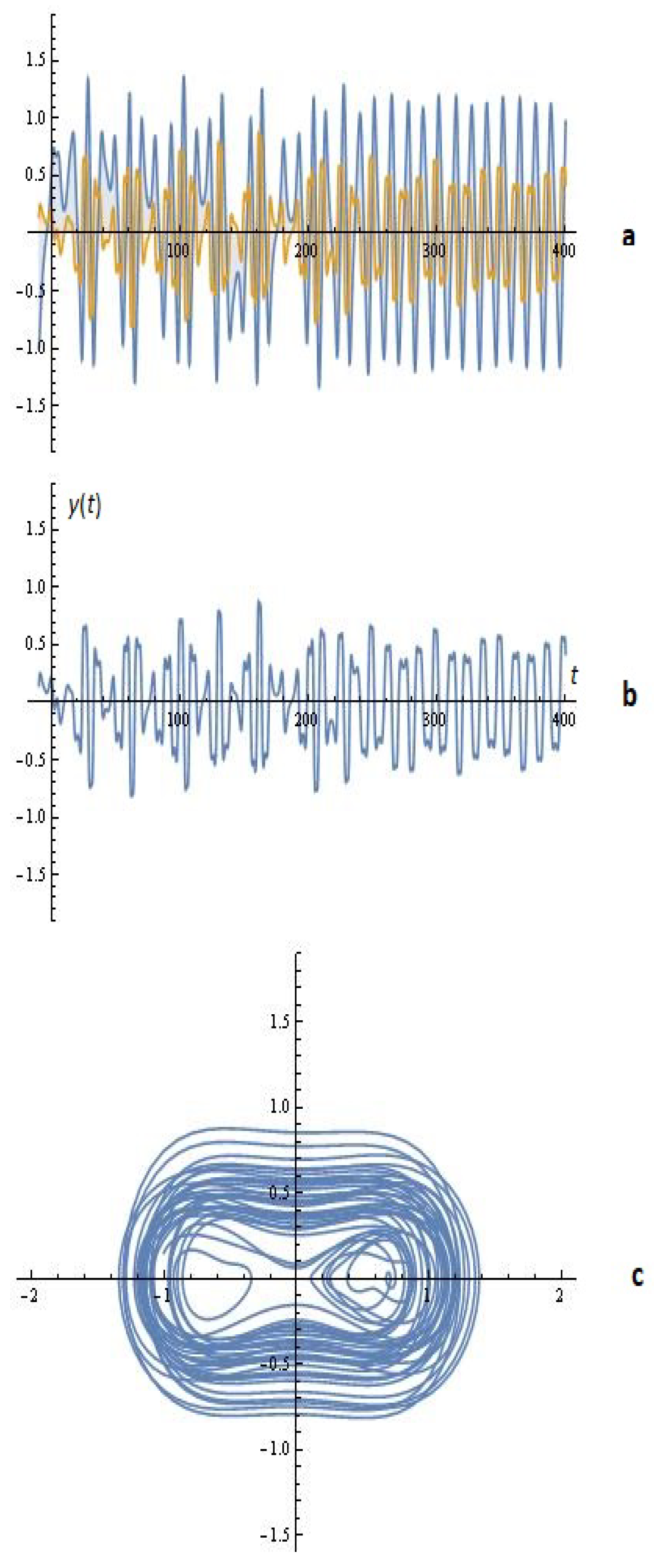
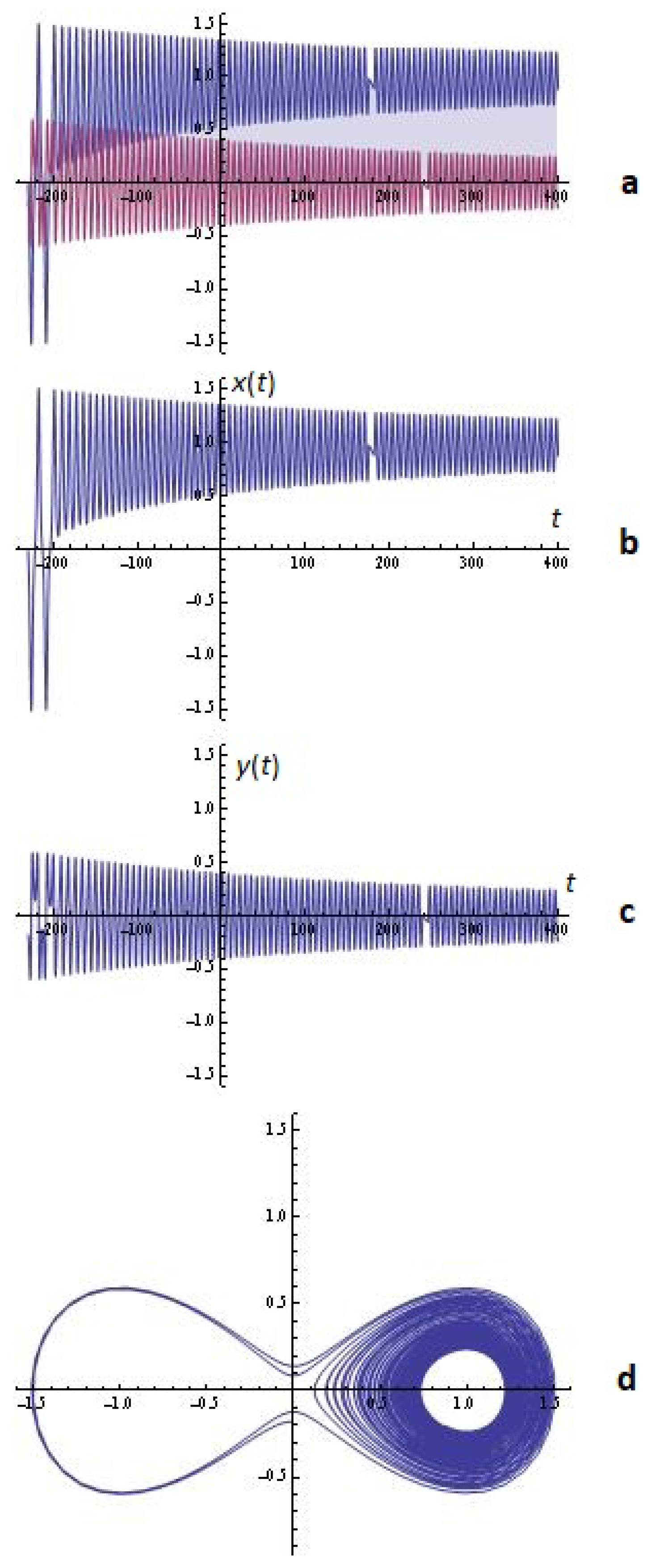
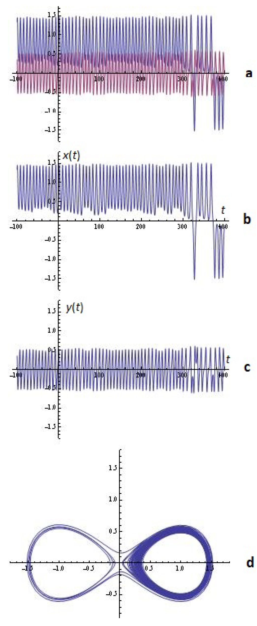
2.1.1. Some Simulations

Let us concentrate on several intriguing examples:

Example 1.

For fixed $b=0.4;b_1=0.7;b_0=-0.1;A=0.1;ϵ=0.1;\omega =1.01;$$a=a_1=a_0=1$, the experiments on Model (9) for $x_0=0.6$; $y_0=0.3$ are visualized in Figure 2.

Example 2.

For fixed $b=0.4;b_1=0.7;b_0=-0.1;A=0.1;ϵ=0.1;\omega =1.01;$$a=0.9;a_1=0.8;a_0=0.7$, the experiments on Model (9) for $x_0=0.6$; $y_0=0.3$ are visualized in Figure 3.

Example 3.

For fixed $b=0.4;b_1=0.7;b_0=-0.1;A=0.01;ϵ=0.1;\omega =1.01;$$a=-0.7;a_1=-3.8;a_0=5.3$, the experiments on Model (9) for $x_0=0.6$; $y_0=0.3$ are visualized in Figure 4.

Example 4.

For fixed $b=0.1;b_1=0.3;b_0=-0.1;A=0.01;ϵ=0.1;\omega =1.01;$$a=-1.7;a_1=-2.8;a_0=6.1$, the experiments on Model (9) for $x_0=0.6$; $y_0=0.2$ are visualized in Figure 5.

2.2. A Modified Model

Let us investigate the next differential system:

$$\left\{\begin{array}{ccc}{\displaystyle \frac{dx}{dt}}\hfill & =& y\hfill \\ {\displaystyle \frac{dy}{dt}}\hfill & =& x-x^3-ϵ\left({Ay\left|y\right|}^{p-1}-{\displaystyle \sum _{j=1}^N}{g}_{j}sin\left(j\omega t\right)\right)\hfill \end{array}\right.$$

(10)

For fixed $ϵ=0$, the outcome Hamiltonian of the model (10) is

$$H(x,y)=\frac{1}{2}{y}^2-\frac{1}{2}{x}^2+\frac{1}{4}{x}^4.$$

A saddle point exists at the origin, which is centered at $(\pm 1,0)$, and a couple homoclinic trajectories are set by (see Figure 6):

$$\begin{array}{c}{x}_0\left(t\right)=\pm \sqrt{2}secht\hfill \\ y_0\left(t\right)=\mp \sqrt{2}sechttanht.\hfill \end{array}$$

(11)

We refer to [8,9,10,11,20] for more details. The homoclinic integral of Melnikov is set by

$$M\left(t_0\right)={\displaystyle {\int }_{-\infty }^{\infty }}{y}_0\left(t\right)\left(A{y}_0\left(t\right){\left|y_0\left(t\right)\right|}^{p-1}-{\displaystyle \sum _{j=1}^N}{g}_{i}sin\left(j\omega (t+t_0)\right)\right)dt,$$

(12)

where the expressions $x_0\left(t\right)$ and $y_0\left(t\right)$ are circumscribed by Equation (11). We will demonstrate the next statement, where $p=2$ and $N=1$.

Proposition 1.

If $p=2$ and $N=1$, then the zeroes of the Melnikov function $M\left(t_0\right)$ are obtained as roots of the following equation:

$$\begin{array}{ccc}M\left(t_0\right)\hfill & =& \frac{16}{15\sqrt{2}}A+\frac{1}{30\sqrt{2}}{e}^{-i{t}_0\omega }\left(15g_1\omega PolyGamma[0,\frac{1}{4}-\frac{i\omega }{4}]\right.\hfill \\ \hfill & & +15e^{2i{t}_0\omega }{g}_1\omega PolyGamma[0,\frac{1}{4}-\frac{i\omega }{4}]-15g_1\omega PolyGamma[0,\frac{3}{4}-\frac{i\omega }{4}]\hfill \\ \hfill & & -15e^{2i{t}_0\omega }{g}_1\omega PolyGamma[0,\frac{3}{4}-\frac{i\omega }{4}]+15g_1\omega PolyGamma[0,\frac{1}{4}+\frac{i\omega }{4}]\hfill \\ \hfill & & +15e^{2i{t}_0\omega }{g}_1\omega PolyGamma[0,\frac{1}{4}+\frac{i\omega }{4}]-15g_1\omega PolyGamma[0,\frac{3}{4}+\frac{i\omega }{4}]\hfill \\ \hfill & & \left.-15e^{2i{t}_0\omega }{g}_1\omega PolyGamma[0,\frac{3}{4}+\frac{i\omega }{4}]\right)=0.\hfill \end{array}$$

(13)

Here, $PolyGamma[n,z]$ is the $n\mathrm{th}$ derivative of the digamma function ${\psi }^{\left(n\right)}\left(z\right)$, i.e., ${\psi }^{\left(0\right)}\left(z\right)=\frac{{\Gamma }^{\prime }\left(z\right)}{\Gamma \left(z\right)}$ and $\Gamma \left(z\right)={\displaystyle {\int }_0^{\infty }}{t}^{z-1}{e}^{-t}dt$ [26].

As an illustration, the equality $M\left(t_0\right)=0$ (for $p=2;N=1;A=1.01;\omega =0.25;$$g_1=0.9$) is depicted in Figure 7a. The roots in interval $(0,26)$ are as follows: $2.42651;$$22.7062$. For $p=2;N=1;A=1.05;\omega =0.1;g_1=0.916$, $M\left(t_0\right)$ has no roots (Figure 7b). From Proposition 1 (see also Figure 7), the reader may formulate the Melnikov’s condition for chaotic behavior of the dynamical model. Let us demonstrate the next statement, where $p=2$ and $N=2$.

Proposition 2.

If $p=2$ and $N=2$, then the zeros of the Melnikov function $M\left(t_0\right)$ are received as roots of the equation

$$\begin{array}{ccc}M\left(t_0\right)\hfill & =& \frac{1}{30\sqrt{2}}{e}^{-2i{t}_0\omega }\left(32A{e}^{2i{t}_0\omega }+15e^{i{t}_0\omega }{g}_1\omega PolyGamma[0,\frac{1}{4}-\frac{i\omega }{4}]\right.\hfill \\ \hfill & & +15e^{3i{t}_0\omega }{g}_1\omega PolyGamma[0,\frac{1}{4}-\frac{i\omega }{4}]-15e^{i{t}_0\omega }{g}_1\omega PolyGamma[0,\frac{3}{4}-\frac{i\omega }{4}]\hfill \\ \hfill & & -15e^{3i{t}_0\omega }{g}_1\omega PolyGamma[0,\frac{3}{4}-\frac{i\omega }{4}]+15e^{i{t}_0\omega }{g}_1\omega PolyGamma[0,\frac{1}{4}+\frac{i\omega }{4}]\hfill \\ \hfill & & +15e^{3i{t}_0\omega }{g}_1\omega PolyGamma[0,\frac{1}{4}+\frac{i\omega }{4}]-15e^{i{t}_0\omega }{g}_1\omega PolyGamma[0,\frac{3}{4}+\frac{i\omega }{4}]\hfill \\ \hfill & & -15e^{3i{t}_0\omega }{g}_1\omega PolyGamma[0,\frac{3}{4}+\frac{i\omega }{4}]+30g_2\omega PolyGamma[0,\frac{1}{4}-\frac{i\omega }{2}]\hfill \\ \hfill & & +30e^{4i{t}_0\omega }{g}_2\omega PolyGamma[0,\frac{1}{4}-\frac{i\omega }{2}]-30g_2\omega PolyGamma[0,\frac{3}{4}-\frac{i\omega }{2}]\hfill \\ \hfill & & -30e^{4i{t}_0\omega }{g}_2\omega PolyGamma[0,\frac{3}{4}-\frac{i\omega }{2}]+30g_2\omega PolyGamma[0,\frac{3}{4}+\frac{i\omega }{2}]\hfill \\ \hfill & & +30e^{4i{t}_0\omega }{g}_2\omega PolyGamma[0,\frac{1}{4}+\frac{i\omega }{2}]-30g_2\omega PolyGamma[0,\frac{3}{4}+\frac{i\omega }{2}]\hfill \\ \hfill & & \left.-30e^{4i{t}_0\omega }{g}_2\omega PolyGamma[0,\frac{3}{4}+\frac{i\omega }{2}]\right)=0.\hfill \end{array}$$

(14)

As an illustration, the equation $M\left(t_0\right)=0$ when (for (a)) $p=2;N=2;$$A=1.01;$$\omega =0.4;g_1=0.4;$$g_2=0.95$ is depicted in Figure 8a. The roots in interval $(0,12)$ are: $1.74485;$$6.92814;$$8.798$. For (b), $p=2;N=2;A=0.6;\omega =0.6;g_1=0.09;g_2=0.05,M\left(t_0\right)$ has no roots (see Figure 8b).

The next proposition is fulfilled for fixed $p=2$ and $N=3$. We will note that this result was reported in [21] only as a particular example illustrating the obstacles that the researcher faces in the usage of a particular CAS. Here, we place it in full.

Proposition 3.

If $p=2$ and $N=3$, then the zeros of the Melnikov function $M\left(t_0\right)$ are obtained as a roots of the following equation:

$$\begin{array}{ccc}M\left(t_0\right)\hfill & =& \frac{1}{60}{e}^{-3i{t}_0\omega }\left(32\sqrt{2}A{e}^{3i{t}_0\omega }+15\sqrt{2}{e}^{2i{t}_0\omega }{g}_1\omega PolyGamma[0,\frac{1}{4}-\frac{i\omega }{4}]\right.\hfill \\ \hfill & & +15\sqrt{2}{e}^{4i{t}_0\omega }{g}_1\omega PolyGamma[0,\frac{1}{4}-\frac{i\omega }{4}]-15\sqrt{2}{e}^{2i{t}_0\omega }{g}_1\omega PolyGamma[0,\frac{3}{4}-\frac{i\omega }{4}]\hfill \\ \hfill & & -15\sqrt{2}{e}^{4i{t}_0\omega }{g}_1\omega PolyGamma[0,\frac{3}{4}-\frac{i\omega }{4}]+15\sqrt{2}{e}^{2i{t}_0\omega }{g}_1\omega PolyGamma[0,\frac{1}{4}+\frac{i\omega }{4}]\hfill \\ \hfill & & +15\sqrt{2}{e}^{4i{t}_0\omega }{g}_1\omega PolyGamma[0,\frac{1}{4}+\frac{i\omega }{4}]-15\sqrt{2}{e}^{2i{t}_0\omega }{g}_1\omega PolyGamma[0,\frac{3}{4}+\frac{i\omega }{4}]\hfill \\ \hfill & & -15\sqrt{2}{e}^{4i{t}_0\omega }{g}_1\omega PolyGamma[0,\frac{3}{4}+\frac{i\omega }{4}]+30\sqrt{2}{e}^{i{t}_0\omega }{g}_2\omega PolyGamma[0,\frac{1}{4}-\frac{i\omega }{2}]\hfill \\ \hfill & & +30\sqrt{2}{e}^{5i{t}_0\omega }{g}_2\omega PolyGamma[0,\frac{1}{4}-\frac{i\omega }{2}]-30\sqrt{2}{e}^{i{t}_0\omega }{g}_2\omega PolyGamma[0,\frac{3}{4}-\frac{i\omega }{2}]\hfill \\ \hfill & & -30\sqrt{2}{e}^{5i{t}_0\omega }{g}_2\omega PolyGamma[0,\frac{3}{4}-\frac{i\omega }{2}]+30\sqrt{2}{e}^{i{t}_0\omega }{g}_2\omega PolyGamma[0,\frac{1}{4}+\frac{i\omega }{2}]\hfill \\ \hfill & & +30\sqrt{2}{e}^{5i{t}_0\omega }{g}_2\omega PolyGamma[0,\frac{1}{4}+\frac{i\omega }{2}]-30\sqrt{2}{e}^{i{t}_0\omega }{g}_2\omega PolyGamma[0,\frac{3}{4}+\frac{i\omega }{2}]\hfill \\ \hfill & & -30\sqrt{2}{e}^{5i{t}_0\omega }{g}_2\omega PolyGamma[0,\frac{3}{4}+\frac{i\omega }{2}]+45\sqrt{2}{g}_3\omega PolyGamma[0,\frac{1}{4}-\frac{3i\omega }{4}]\hfill \\ \hfill & & +45\sqrt{2}{e}^{6i{t}_0\omega }{g}_3\omega PolyGamma[0,\frac{1}{4}-\frac{3i\omega }{4}]-45\sqrt{2}{g}_3\omega PolyGamma[0,\frac{3}{4}-\frac{3i\omega }{4}]\hfill \\ \hfill & & -45\sqrt{2}{e}^{6i{t}_0\omega }{g}_3\omega PolyGamma[0,\frac{3}{4}-\frac{3i\omega }{4}]+45\sqrt{2}{g}_3\omega PolyGamma[0,\frac{1}{4}+\frac{3i\omega }{4}]\hfill \\ \hfill & & +45\sqrt{2}{e}^{6i{t}_0\omega }{g}_3\omega PolyGamma[0,\frac{1}{4}+\frac{3i\omega }{4}]-45\sqrt{2}{g}_3\omega PolyGamma[0,\frac{3}{4}+\frac{3i\omega }{4}]\hfill \\ \hfill & & \left.-45\sqrt{2}{e}^{6i{t}_0\omega }{g}_3\omega PolyGamma[0,\frac{3}{4}+\frac{3i\omega }{4}]\right)=0.\hfill \end{array}$$

(15)

As an illustration, the equation $M\left(t_0\right)=0$ when (a) $p=2;N=3;A=1.01;$$\omega =0.34;g_1=0.5;g_2=0.95;g_3=0.8$ is visualized in Figure 9a. For (b), $p=2;$$N=3;A=0.1;\omega =0.9;$$g_1=0.01;g_2=0.02;g_3=0.015,M\left(t_0\right)$ has no roots (see Figure 9b).

From Propositions 2 and 3, the reader may formulate the Melnikov’s standard for the emergence of crossing the perturbed and unperturbed separatrix. The reader can explore the relevant approximation issue for arbitrarily selected p and N.

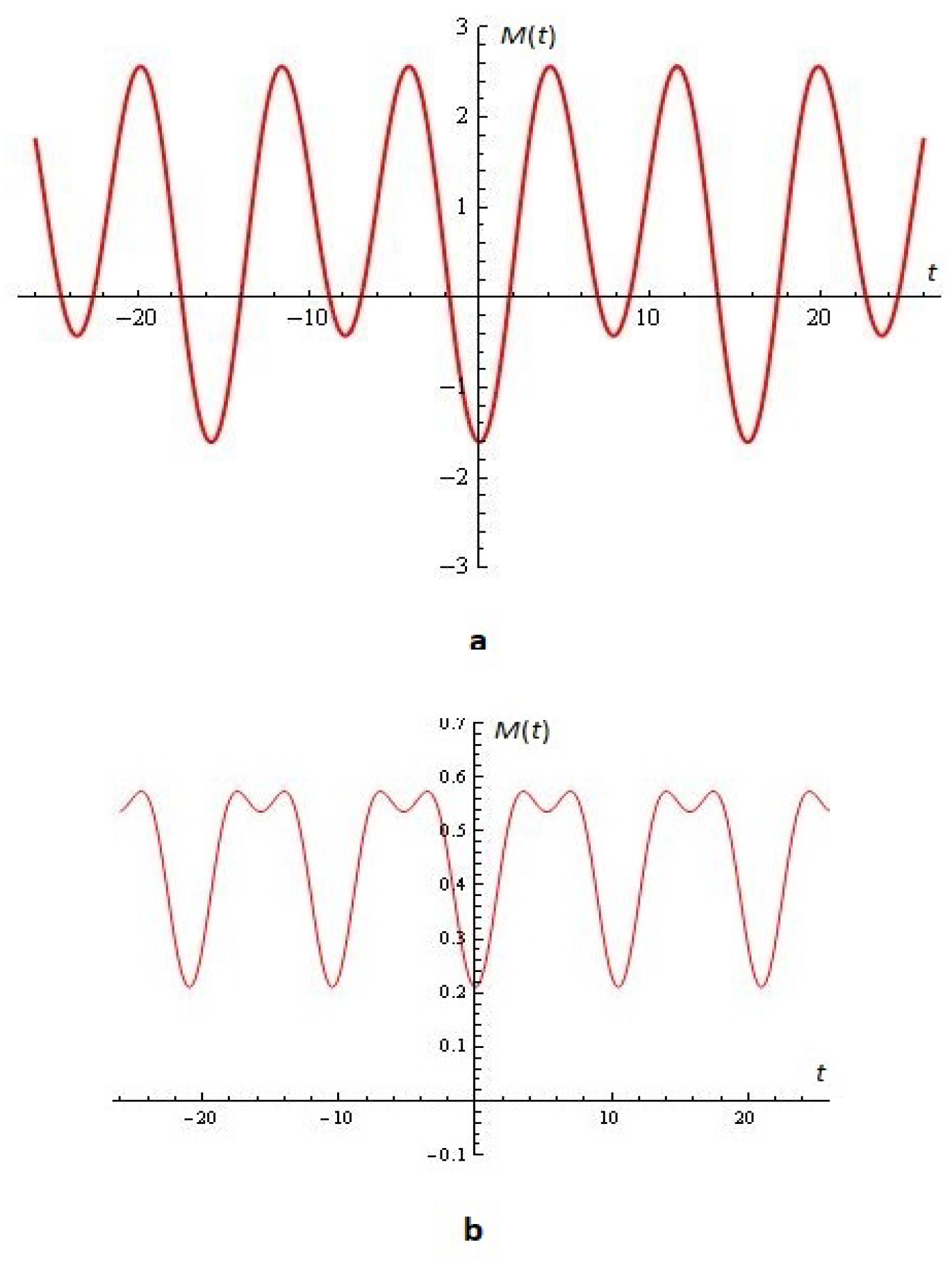
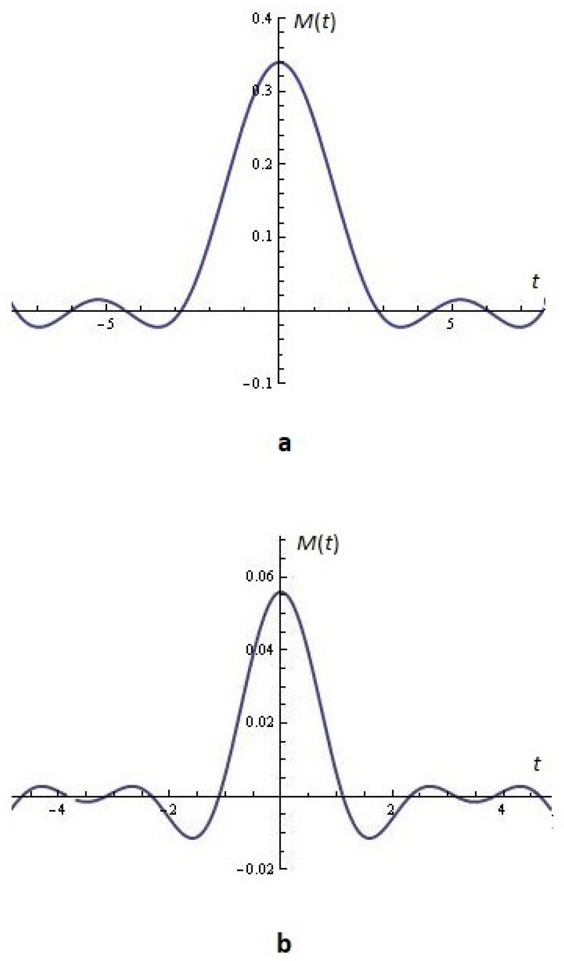
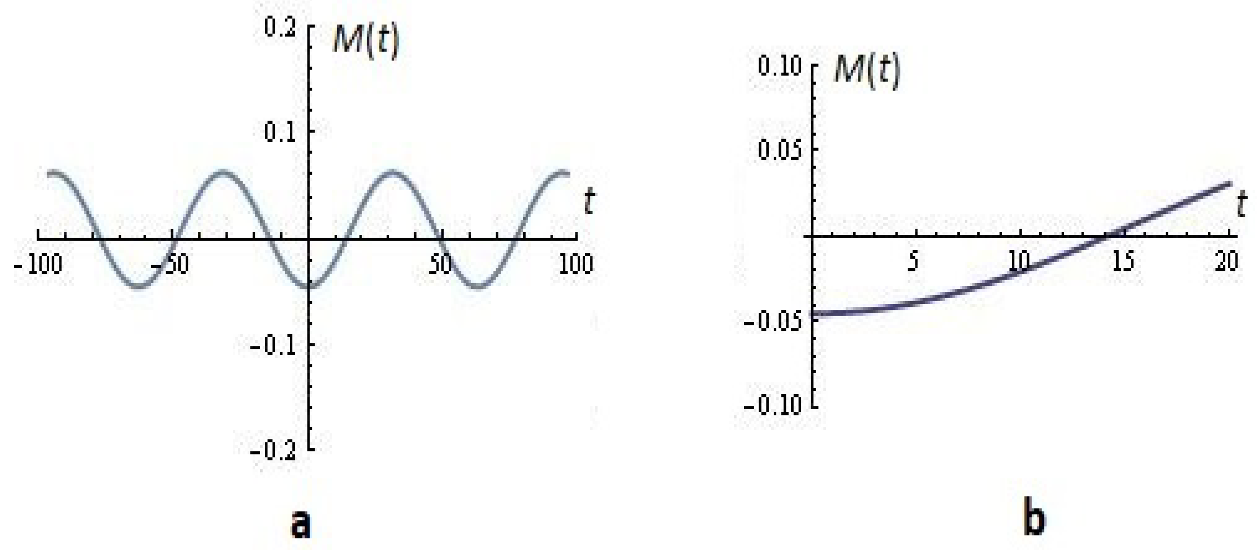
2.3. One Possible Application That Melnikov Functions May Find in the Modeling and Synthesis of Radiating Antenna Patterns

Let us dwell on the functions $M\left(t\right)$ generated by Propositions 2 and 3. Thus, for example, typical diagrams are visualized in Figure 10 with the following selection of parameters:

I.

$p=2;N=2;A=0.13;\omega =0.6;g_1=-0.09;g_2=-0.05$ (from Proposition 2);

II.

$p=2;N=3;A=0.011;\omega =0.9;g_1=-0.01;g_2=-0.02;g_3=-0.03$ (from Proposition 3).

Of course, the complex problem related to choosing an optimization approach to minimize lateral radiation in the specified class of diagrams can be considered as open.

The reader can find additional information in [27].

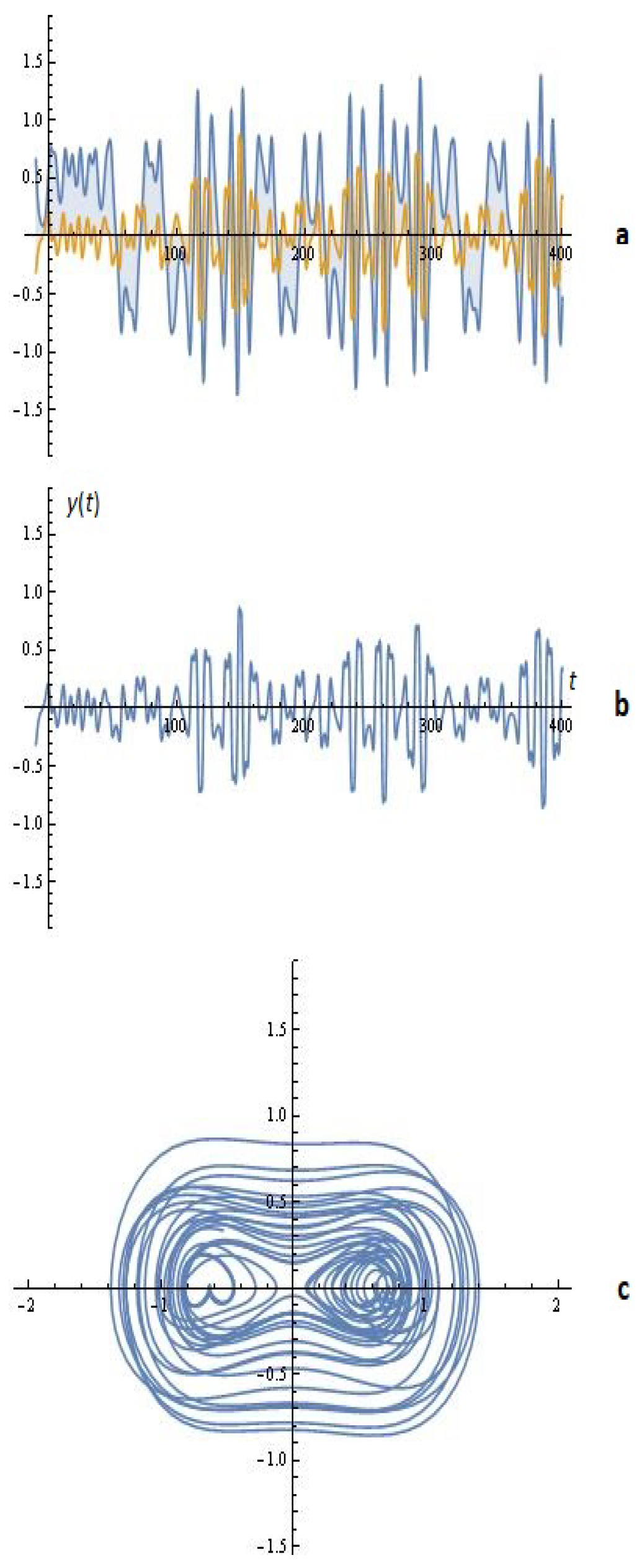
3. One More Note on the Subject: Generating Chaos via $\mathit{x}\left|\mathit{x}\right|$

In this section, we will explore the dynamics of the following ”mixed” model:

$$\left\{\begin{array}{ccc}{\displaystyle \frac{dx}{dt}}\hfill & =& y\hfill \\ {\displaystyle \frac{dy}{dt}}\hfill & =& x-x\left|x\right|-ϵ\left(A{\displaystyle \sum _{p=1}^n}y{\left|y\right|}^{p-1}-{\displaystyle \sum _{j=1}^N}{g}_{j}sin\left(j\omega t\right)\right)\hfill \end{array}\right.$$

(16)

where $0\le ϵ<1$, A is the damping level, N is natural number, and $p\ge 1$ is the damping exponent. Particularly, we investigate the next differential system

$$\left\{\begin{array}{ccc}{\displaystyle \frac{dx}{dt}}\hfill & =& y\hfill \\ {\displaystyle \frac{dy}{dt}}\hfill & =& x-x\left|x\right|-ϵ\left({Ay\left|y\right|}^{p-1}-{\displaystyle \sum _{j=1}^N}{g}_{j}sin\left(j\omega t\right)\right).\hfill \end{array}\right.$$

(17)

The total energy of this system ($ϵ=0$) is $H(x,y)=\frac{1}{2}{y}^2-\frac{1}{2}{x}^2+\frac{1}{3}{x}^2\left|x\right|$. Some details can be found in [13]. The trajectory is obtained by (see Figure 11):

$$\begin{array}{ccc}{x}_0\left(t\right)\hfill & =& \pm \frac{3}{1+cosh\dot{t}}\hfill \\ y_0\left(t\right)\hfill & =& \mp \frac{3sinht}{{(1+cosh\dot{t})}^2}\hfill \end{array}$$

(18)

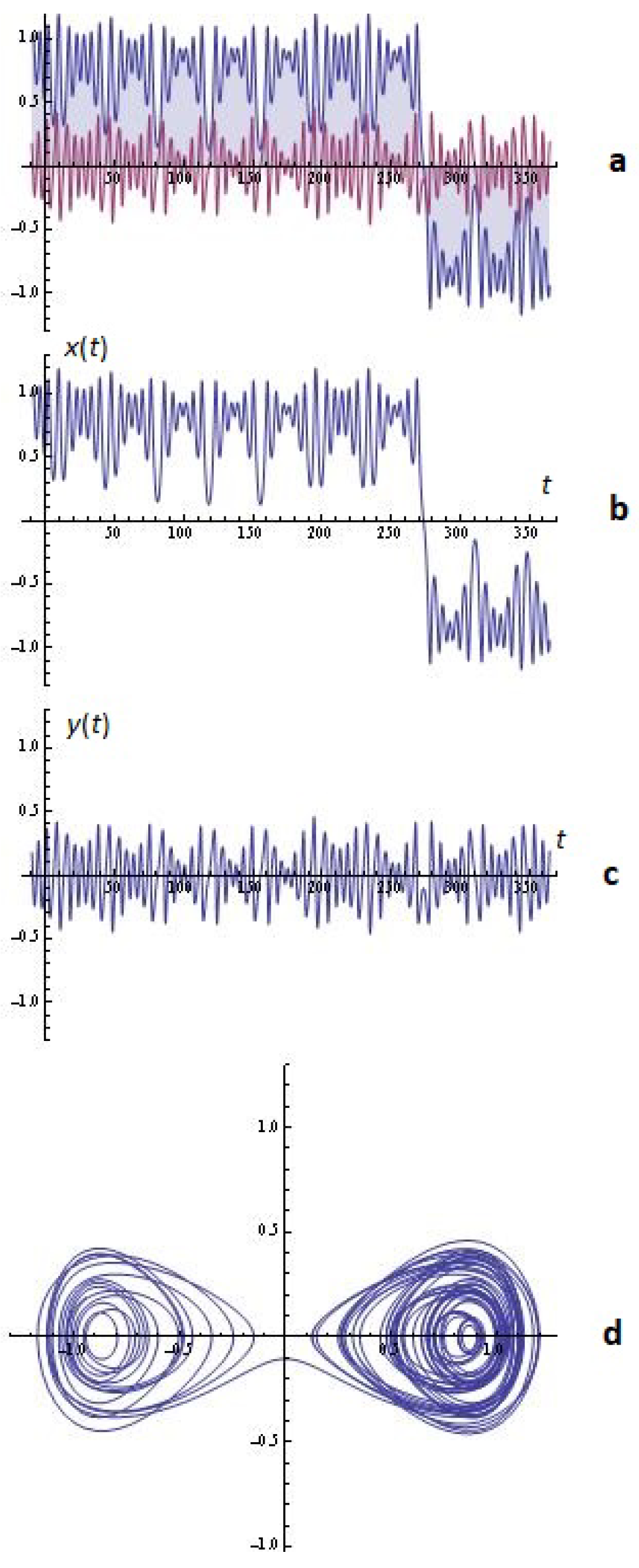
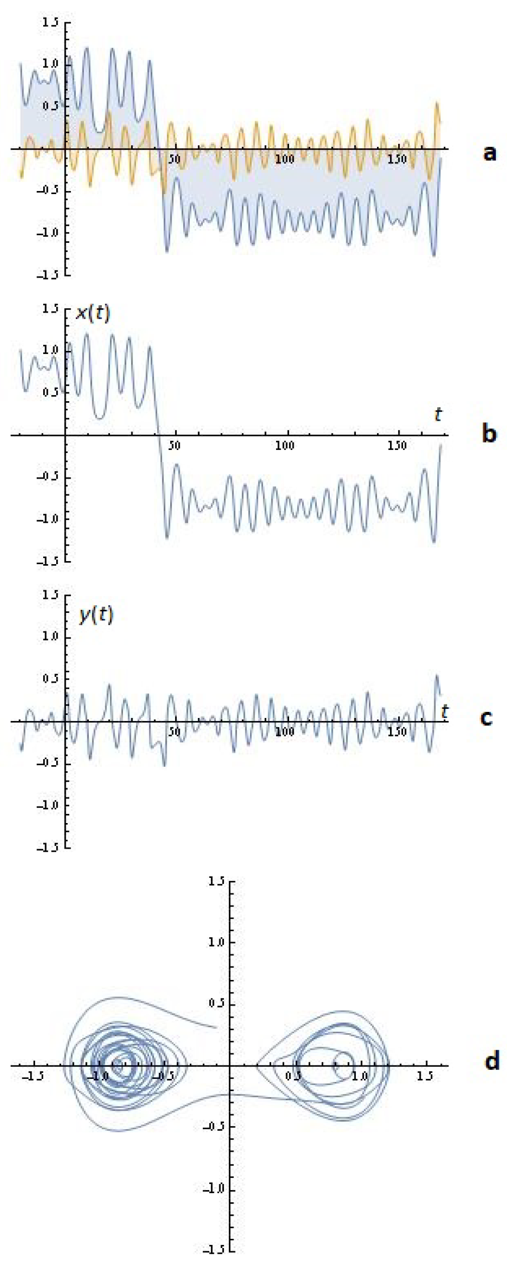
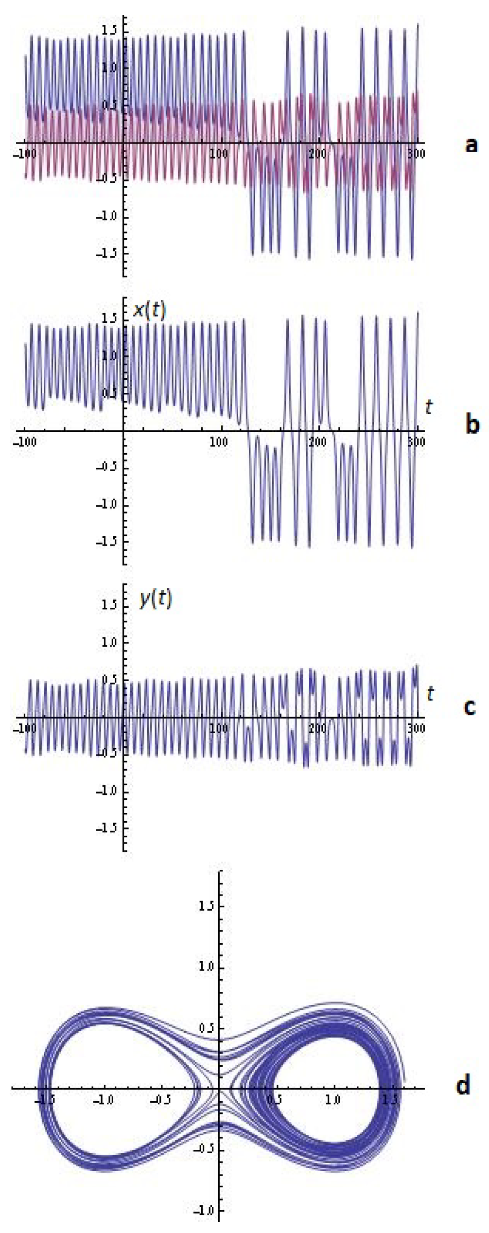
3.1. Some Simulations

Let us consider several intriguing experiments:

Example 5.

For fixed $p=2;N=2;A=0.015;ϵ=0.1;\omega =0.6;g_1=0.07;g_2=0.3$, the experiments by Model (17) for $x_0=0.6$; $y_0=0.2$ are visualized in Figure 12.

Example 6.

For fixed $p=6;N=3;A=0.1;ϵ=0.1;\omega =0.32;g_1=0.9;g_2=0.8;g_3=0.7$, the experiments by Model (17) for $x_0=0.8$; $y_0=0.5$ are visualized in Figure 13.

Example 7.

For fixed $p=8;N=5;A=0.1;ϵ=0.1;\omega =0.32;g_1=0.9;g_2=0.8;$$g_3=0.7;g_4=0.6;g_5=0.5$, the experiments by Model (17) for $x_0=0.6$; $y_0=0.3$ are visualized in Figure 14.

Example 8.

For fixed $p=10;N=6;A=0.1;ϵ=0.1;\omega =0.32;g_1=0.9;g_2=0.1;$$g_3=0.8;g_4=0.2;g_5=0.7;g_6=0$, the experiments by Model (17) for $x_0=0.7$; $y_0=0.5$ are visualized in Figure 15.

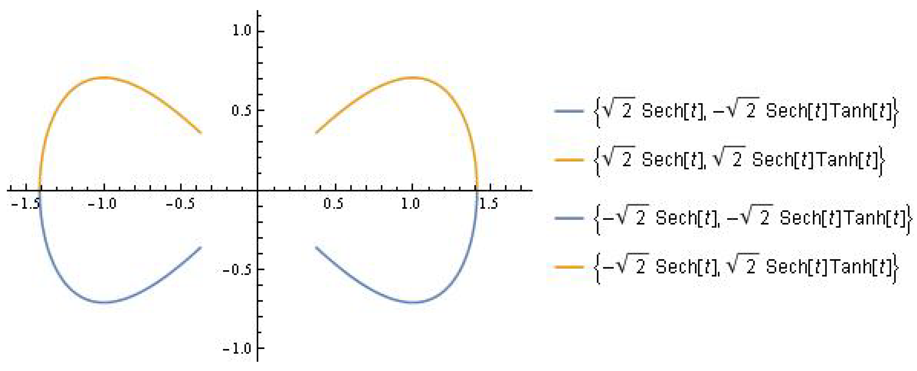
3.1.1. Melnikov’s Approach

By definition, the Melnikov integral is presented by

$$M\left(t_0\right)={\displaystyle {\int }_{-\infty }^{\infty }}{y}_0\left(t\right)\left(A{y}_0\left(t\right){\left|y_0\left(t\right)\right|}^{p-1}-{\displaystyle \sum _{j=1}^N}{g}_{i}sin\left(j\omega (t+t_0)\right)\right)dt,$$

(19)

where the functions $x_0\left(t\right)$ and $y_0\left(t\right)$ are defined by Equation (18).

Let us indicate the next statement for fixed $p=2$ and $N=1$.

Proposition 4.

If $p=2$ and $N=1$, then the zeroes of the Melnikov function $M\left(t_0\right)$ are received as roots of the following equation:

$$\begin{array}{c}M\left(t_0\right)=\frac{1}{\mathrm{75,600}}{e}^{-it0\omega }\left(\mathrm{42,525}A{e}^{it0\omega }-\mathrm{226,800}g1\omega -\mathrm{226,800}{e}^{2it0\omega }g1\omega +\mathrm{188,016}g1{\omega }^3\right.\hfill \\ +\mathrm{188,016}{e}^{2it0\omega }g1{\omega }^3-\mathrm{37,328}g1{\omega }^5-\mathrm{37,328}{e}^{2it0\omega }g1{\omega }^5+2144g1{\omega }^7+2144e^{2it0\omega }g1{\omega }^7\hfill \\ -32g1{\omega }^9-32e^{2it0\omega }g1{\omega }^9+\mathrm{62,136}ig1{\omega }^{2}P[0,\frac{1}{2}-\frac{i\omega }{2}]+\mathrm{62,136}i{e}^{2it0\omega }g1{\omega }^{2}P[0,\frac{1}{2}-\frac{i\omega }{2}]\hfill \\ -\mathrm{45,800}ig1{\omega }^{4}P[0,\frac{1}{2}-\frac{i\omega }{2}]-\mathrm{45,800}i{e}^{2it0\omega }g1{\omega }^{4}P[0,\frac{1}{2}-\frac{I\omega }{2}]+5313ig1{\omega }^{6}P[0,\frac{1}{2}-\frac{i\omega }{2}]\hfill \\ +5313i{e}^{2it0\omega }g1{\omega }^{6}P[0,\frac{1}{2}-\frac{i\omega }{2}]-150ig1{\omega }^{8}P[0,\frac{1}{2}-\frac{I\omega }{2}]-150i{e}^{2it0\omega }g1{\omega }^{8}P[0,\frac{1}{2}-\frac{i\omega }{2}]\hfill \\ +ig1{\omega }^{10}P[0,\frac{1}{2}-\frac{i\omega }{2}]+i{e}^{2it0\omega }g1{\omega }^{10}P[0,\frac{1}{2}-\frac{i\omega }{2}]-\mathrm{94,392}ig1{\omega }^{2}P[0,1-\frac{i\omega }{2}]\hfill \\ -\mathrm{94,392}i{e}^{2it0\omega }g1{\omega }^{2}P[0,1-\frac{i\omega }{2}]+\mathrm{22,620}ig1{\omega }^{4}P[0,1-\frac{i\omega }{2}]+\mathrm{22,620}i{e}^{2it0\omega }g1{\omega }^{4}P[0,1-\frac{i\omega }{2}]\hfill \\ +3339ig1{\omega }^{6}P[0,1-\frac{i\omega }{2}]+3339i{e}^{2it0\omega }g1{\omega }^{6}P[0,1-\frac{i\omega }{2}]-270ig1{\omega }^{8}P[0,1-\frac{i\omega }{2}]\hfill \\ -270i{e}^{2it0\omega }g1{\omega }^{8}P[0,1-\frac{i\omega }{2}]+3ig1{\omega }^{10}P[0,1-\frac{i\omega }{2}]+3i{e}^{2it0\omega }g1{\omega }^{10}P[0,1-\frac{i\omega }{2}]\hfill \\ +\mathrm{46,512}ig1{\omega }^{2}P[0,\frac{3}{2}-\frac{i\omega }{2}]+\mathrm{46,512}i{e}^{2it0\omega }g1{\omega }^{2}P[0,\frac{3}{2}-\frac{i\omega }{2}]+\mathrm{39,440}ig1{\omega }^{4}P[0,\frac{3}{2}-\frac{i\omega }{2}]\hfill \\ +\mathrm{39,440}i{e}^{2it0\omega }g1{\omega }^{4}P[0,\frac{3}{2}-\frac{i\omega }{2}]-7014ig1{\omega }^{6}P[0,\frac{3}{2}-\frac{i\omega }{2}]-7014i{e}^{2it0\omega }g1{\omega }^{6}P[0,\frac{3}{2}-\frac{i\omega }{2}]\hfill \\ +60ig1{\omega }^{8}P[0,\frac{3}{2}-\frac{i\omega }{2}]+60i{e}^{2it0\omega }g1{\omega }^{8}P[0,\frac{3}{2}-\frac{i\omega }{2}]+2ig1{\omega }^{10}P[0,\frac{3}{2}-\frac{i\omega }{2}]\hfill \\ +2i{e}^{2it0\omega }g1{\omega }^{10}P[0,\frac{3}{2}-\frac{i\omega }{2}]-\mathrm{18,432}ig1{\omega }^{2}P[0,2-\frac{i\omega }{2}]-\mathrm{18,432}i{e}^{2it0\omega }g1{\omega }^{2}P[0,2-\frac{i\omega }{2}]\hfill \\ -\mathrm{21,800}ig1{\omega }^{4}P[0,2-\frac{i\omega }{2}]-\mathrm{21,800}i{e}^{2it0\omega }g1{\omega }^{4}P[0,2-\frac{i\omega }{2}]-3066ig1{\omega }^{6}P[0,2-\frac{i\omega }{2}]\hfill \\ -3066i{e}^{2it0\omega }g1{\omega }^{6}P[0,2-\frac{i\omega }{2}]+300ig1{\omega }^{8}P[0,2-\frac{i\omega }{2}]+300i{e}^{2it0\omega }g1{\omega }^{8}P[0,2-\frac{i\omega }{2}]\hfill \\ -2ig1{\omega }^{10}P[0,2-\frac{i\omega }{2}]-2i{e}^{2it0\omega }g1{\omega }^{10}P[0,2-\frac{i\omega }{2}]+4752ig1{\omega }^{2}P[0,\frac{5}{2}-\frac{i\omega }{2}]\hfill \\ +4752i{e}^{2it0\omega }g1{\omega }^{2}P[0,\frac{5}{2}-\frac{i\omega }{2}]+6360Ig1{\omega }^{4}P[0,\frac{5}{2}-\frac{i\omega }{2}]+6360i{e}^{2it0\omega }g1{\omega }^{4}P[0,\frac{5}{2}-\frac{i\omega }{2}]\hfill \\ +1701ig1{\omega }^{6}P[0,\frac{5}{2}-\frac{i\omega }{2}]+1701i{e}^{2it0\omega }g1{\omega }^{6}P[0,\frac{5}{2}-\frac{i\omega }{2}]+90ig1{\omega }^{8}P[0,\frac{5}{2}-\frac{i\omega }{2}]\hfill \\ +90i{e}^{2it0\omega }g1{\omega }^{8}P[0,\frac{5}{2}-\frac{i\omega }{2}]-3ig1{\omega }^{10}P[0,\frac{5}{2}-\frac{i\omega }{2}]-3i{e}^{2it0\omega }g1{\omega }^{10}P[0,\frac{5}{2}-\frac{I\omega }{2}]\hfill \\ -576ig1{\omega }^{2}P[0,3-\frac{I\omega }{2}]-576i{e}^{2it0\omega }g1{\omega }^{2}P[0,3-\frac{i\omega }{2}]-820ig1{\omega }^{4}P[0,3-\frac{i\omega }{2}]\hfill \\ -820i{e}^{2it0\omega }g1{\omega }^{4}P[0,3-\frac{i\omega }{2}]-273ig1{\omega }^{6}P[0,3-\frac{i\omega }{2}]-273i{e}^{2it0\omega }g1{\omega }^{6}P[0,3-\frac{i\omega }{2}]\hfill \\ -30ig1{\omega }^{8}P[0,3-\frac{i\omega }{2}]-30i{e}^{2it0\omega }g1{\omega }^{8}P[0,3-\frac{i\omega }{2}]-ig1{\omega }^{10}P[0,3-\frac{i\omega }{2}]\hfill \\ -i{e}^{2it0\omega }g1{\omega }^{10}P[0,3-\frac{i\omega }{2}]-\mathrm{62,136}ig1{\omega }^{2}P[0,\frac{1}{2}+\frac{i\omega }{2}]-\mathrm{62,136}i{e}^{2it0\omega }g1{\omega }^{2}P[0,\frac{1}{2}+\frac{i\omega }{2}]\hfill \\ +\mathrm{45,800}ig1{\omega }^{4}P[0,\frac{1}{2}+\frac{i\omega }{2}]+\mathrm{45,800}i{e}^{2it0\omega }g1{\omega }^{4}P[0,\frac{1}{2}+\frac{i\omega }{2}]-5313ig1{\omega }^{6}P[0,\frac{1}{2}+\frac{i\omega }{2}]\hfill \\ -5313i{e}^{2it0\omega }g1{\omega }^{6}P[0,\frac{1}{2}+\frac{i\omega }{2}]+150ig1{\omega }^{8}P[0,\frac{1}{2}+\frac{i\omega }{2}]+150i{e}^{2it0\omega }g1{\omega }^{8}P[0,\frac{1}{2}+\frac{i\omega }{2}]\hfill \\ -ig1{\omega }^{10}P[0,\frac{1}{2}+\frac{i\omega }{2}]-i{e}^{2it0\omega }g1{\omega }^{10}P[0,\frac{1}{2}+\frac{i\omega }{2}]+\mathrm{94,392}ig1{\omega }^{2}P[0,1+\frac{i\omega }{2}]\hfill \\ +\mathrm{94,392}i{e}^{2it0\omega }g1{\omega }^{2}P[0,1+\frac{i\omega }{2}]-22,620ig1{\omega }^{4}P[0,1+\frac{i\omega }{2}]-\mathrm{22,620}i{e}^{2it0\omega }g1{\omega }^{4}P[0,1+\frac{i\omega }{2}]\hfill \\ -3339ig1{\omega }^{6}P[0,1+\frac{i\omega }{2}]-3339i{e}^{2it0\omega }g1{\omega }^{6}P[0,1+\frac{i\omega }{2}]+270ig1{\omega }^{8}P[0,1+\frac{i\omega }{2}]\hfill \\ +270i{e}^{2it0\omega }g1{\omega }^{8}P[0,1+\frac{i\omega }{2}]-3ig1{\omega }^{10}P[0,1+\frac{i\omega }{2}]-3i{e}^{2it0\omega }g1{\omega }^{10}P[0,1+\frac{i\omega }{2}]\hfill \\ -\mathrm{46,512}ig1{\omega }^{2}P[0,\frac{3}{2}+\frac{i\omega }{2}]-\mathrm{46,512}i{e}^{2it0\omega }g1{\omega }^{2}P[0,\frac{3}{2}+\frac{i\omega }{2}]-\mathrm{39,440}ig1{\omega }^{4}P[0,\frac{3}{2}+\frac{i\omega }{2}]\hfill \\ -\mathrm{39,440}i{e}^{2it0\omega }g1{\omega }^{4}P[0,\frac{3}{2}+\frac{i\omega }{2}]+7014ig1{\omega }^{6}P[0,\frac{3}{2}+\frac{i\omega }{2}]+7014i{e}^{2it0\omega }g1{\omega }^{6}P[0,\frac{3}{2}+\frac{i\omega }{2}]\hfill \\ -60ig1{\omega }^{8}P[0,\frac{3}{2}+\frac{i\omega }{2}]-60i{e}^{2it0\omega }g1{\omega }^{8}P[0,\frac{3}{2}+\frac{i\omega }{2}]-2ig1{\omega }^{10}P[0,\frac{3}{2}+\frac{i\omega }{2}]\hfill \\ -2i{e}^{2it0\omega }g1{\omega }^{10}P[0,\frac{3}{2}+\frac{i\omega }{2}]+\mathrm{18,432}ig1{\omega }^{2}P[0,2+\frac{i\omega }{2}]+\mathrm{18,432}i{e}^{2it0\omega }g1{\omega }^{2}P[0,2+\frac{i\omega }{2}]\hfill \\ +\mathrm{21,800}ig1{\omega }^{4}P[0,2+\frac{i\omega }{2}+\mathrm{21,800}i{e}^{2it0\omega }g1{\omega }^{4}P[0,2+\frac{i\omega }{2}]+3066ig1{\omega }^{6}P[0,2+\frac{i\omega }{2}]\hfill \\ +3066i{e}^{2it0\omega }g1{\omega }^{6}P[0,2+\frac{i\omega }{2}]-300iIg1{\omega }^{8}P[0,2+\frac{i\omega }{2}]-300i{e}^{2it0\omega }g1{\omega }^{8}P[0,2+\frac{i\omega }{2}]\hfill \\ +2ig1{\omega }^{10}P[0,2+\frac{i\omega }{2}]+2i{e}^{2it0\omega }g1{\omega }^{10}P[0,2+\frac{i\omega }{2}]-4752ig1{\omega }^{2}P[0,\frac{5}{2}+\frac{i\omega }{2}]\hfill \\ -4752i{e}^{2it0\omega }g1{\omega }^{2}P[0,\frac{5}{2}+\frac{i\omega }{2}]-6360ig1{\omega }^{4}P[0,\frac{5}{2}+\frac{i\omega }{2}]-6360i{e}^{2it0\omega }g1{\omega }^{4}P[0,\frac{5}{2}+\frac{i\omega }{2}]\hfill \\ -1701ig1{\omega }^{6}P[0,\frac{5}{2}+\frac{i\omega }{2}]-1701i{e}^{2it0\omega }g1{\omega }^{6}P[0,\frac{5}{2}+\frac{i\omega }{2}]-90ig1{\omega }^{8}P[0,\frac{5}{2}+\frac{i\omega }{2}]\hfill \\ -90i{e}^{2it0\omega }g1{\omega }^{8}P[0,\frac{5}{2}+\frac{i\omega }{2}]+3ig1{\omega }^{10}P[0,\frac{5}{2}+\frac{i\omega }{2}]+3i{e}^{2it0\omega }g1{\omega }^{10}P[0,\frac{5}{2}+\frac{i\omega }{2}]\hfill \\ +576ig1{\omega }^{2}P[0,3+\frac{i\omega }{2}]+576i{e}^{2it0\omega }g1{\omega }^{2}P[0,3+\frac{i\omega }{2}]+820iIg1{\omega }^{4}P[0,3+\frac{i\omega }{2}]\hfill \\ +820i{e}^{2it0\omega }g1{\omega }^{4}P[0,3+\frac{i\omega }{2}]+273ig1{\omega }^{6}P[0,3+\frac{i\omega }{2}]+273i{e}^{2it0\omega }g1{\omega }^{6}P[0,3+\frac{i\omega }{2}]\hfill \\ +30ig1{\omega }^{8}P[0,3+\frac{i\omega }{2}]+30i{e}^{2it0\omega }g1{\omega }^{8}P[0,3+\frac{i\omega }{2}]+ig1{\omega }^{10}P[0,3+\frac{i\omega }{2}]\hfill \\ \left.+i{e}^{2it0\omega }g1{\omega }^{10}P[0,3+\frac{i\omega }{2}])\right)=0.\hfill \end{array}$$

(20)

Here, we have used the abbreviation $P[.,.]$ instead of $PolyGamma[.,.]$.

Remark 1.

Proposition 4 is generated using direct reference to the specialized module provided in CAS Mathematica; we place it in this form. For the equation $M\left(t_0\right)=0$ (for fixed $A=0.15;$$\omega =0.1;g_1=0.091$), see Figure 16.

4. Some Probability-Based Constructions

Many works devoted to the oscillators with stochastic elements (Gaussian colored noise, Ornstein–Uhlenbeck process, Poisson distribution, different non-Gaussian terms, maximum entropy principle, etc.) are available in the scientific literature—we refer to [28,29,30,31,32]. Despite their different essences, these elements modify the oscillator behavior. We suggest an alternative approach in this research. We assume that the parameters $a_i$ and $b_i$, that control the oscillator dynamics, are generated by some distribution. This way, the intrinsic properties of the used stochastic component can be incorporated into the behavior of the related oscillator; in this way, they improve its fine structure.

Suppose now that the coefficients $a_i$ and $b_i$ from Equation (8) are the probabilities of some finite-space discrete distributions. Let us denote by ${\psi }^a\left(·\right)$ and ${\psi }^b\left(·\right)$ their moment-generating functions. Let ${\xi }_a$ and ${\xi }_b$ be some random variables exhibiting the corresponding laws. We shall use the symbol $\mathbb{E}$ for the related expectations. We can rewrite the second part of system (8) as

$$\begin{array}{cc}\hfill & {\displaystyle \frac{dy}{dt}}=bx-{\displaystyle \sum _{i=0}^{\left[\frac{n}{2}\right]-1}}{b}_i{x}^{n-2i}-ϵ\left(A{\displaystyle \sum _{p=1}^k}y{\left|y\right|}^{2p-1}+(1+cos\left(\omega t\right))\left(ax+{\displaystyle \sum _{i=0}^{\left[\frac{m}{2}\right]-1}}{a}_i{x}^{m-2i}\right)\right)\hfill \\ \hfill & =bx-x^n{\displaystyle \sum _{i=0}^{\left[\frac{n}{2}\right]-1}}{b}_i{e}^{-2iln\left|x\right|}-ϵ\left(A{\displaystyle \sum _{p=1}^k}y{\left|y\right|}^{2p-1}+(1+cos\left(\omega t\right))\left(ax+{\displaystyle x^m\sum _{i=0}^{\left[\frac{m}{2}\right]-1}}{a}_i{e}^{-2iln\left|x\right|}\right)\right)\hfill \\ \hfill & =bx-x^n\mathbb{E}\left[e^{-2{\xi }_{b}ln\left|x\right|}\right]-ϵ\left(A{\displaystyle \sum _{p=1}^k}y{\left|y\right|}^{2p-1}+(1+cos\left(\omega t\right))\left(ax+\mathbb{E}\left[e^{-2{\xi }_{a}ln\left|x\right|}\right]\right)\right)\hfill \\ \hfill & =bx-x^n{\psi }_b\left(-2ln\left|x\right|\right)-ϵ\left(A{\displaystyle \sum _{p=1}^k}y{\left|y\right|}^{2p-1}+(1+cos\left(\omega t\right))\left(ax+{\psi }_a\left(-2ln\left|x\right|\right)\right)\right).\hfill \end{array}$$

(21)

Let us discuss some examples—discrete uniform, binomial, $\beta$-binomial, and hypergeometric distributions. We state the domain at the set $\left\{0,1,2,\dots ,K\right\}$. We have $K=\left[\frac{m}{2}\right]$ for ${\xi }_a$ and $K=\left[\frac{n}{2}\right]$ for ${\xi }_b$, respectively, for $a_i$ and $b_i$. The coefficients $a_i$ and $b_i$ are defined as the probabilities:

$$\begin{array}{cc}\hfill p_i^{\mathrm{uniform}}& =\frac{1}{K}\hfill \\ \hfill p_i^{\mathrm{binomial}}& =\left(\genfrac{}{}{0pt}{}{k}{i}\right)p^i{\left(1-p\right)}^{K-i}\hfill \\ \hfill p_i^{\beta -\mathrm{binomial}}& =\left(\genfrac{}{}{0pt}{}{K}{i}\right)\frac{B\left(i+\alpha ,k-i+\beta \right)}{B\left(\alpha ,\beta \right)}\hfill \\ \hfill p_i^{\mathrm{hypergeometric}}& =\frac{\left(\genfrac{}{}{0pt}{}{K}{i}\right)\left(\genfrac{}{}{0pt}{}{N-K}{M-i}\right)}{\left(\genfrac{}{}{0pt}{}{N}{M}\right)}.\hfill \end{array}$$

(22)

The necessary conditions are $0<p<1$, $\alpha >0$, $\beta >0$, $K\le M\le \left[\frac{N}{2}\right]$, and M and N are integers. The $\beta$-function $B\left(·,·\right)$ is defined through the gamma function as

$$B\left(x,y\right)=\frac{\Gamma \left(x\right)\Gamma \left(y\right)}{\Gamma \left(x+y\right)}.$$

(23)

Having in mind that the moment-generating functions of these distributions are

$$\begin{array}{cc}\hfill {\psi }^{\mathrm{uniform}}\left(x\right)& =\frac{1-e^{\left(K+1\right)x}}{K\left(1-e^x\right)}\hfill \\ \hfill {\psi }^{\mathrm{binomial}}\left(x\right)& ={\left(1-p+p{e}^x\right)}^K\hfill \\ \hfill {\psi }^{\beta -\mathrm{binomial}}\left(x\right)& ={}_{2}F_1\left(-K,\alpha ,\alpha +\beta ,1-e^x\right)\hfill \\ \hfill {\psi }^{\mathrm{hypergeometric}}\left(x\right)& =\frac{\left(\genfrac{}{}{0pt}{}{N-K}{M}\right){}_{2}F_1\left(-M,-K,N-M-K+1,e^x\right)}{\left(\genfrac{}{}{0pt}{}{N}{M}\right)},\hfill \end{array}$$

(24)

we express the terms $\psi \left(-2ln\left|x\right|\right)$ from Equation (21) as

$$\begin{array}{cc}\hfill {\psi }^{\mathrm{uniform}}\left(-2ln\left|x\right|\right)& =\frac{x^{2\left(k+1\right)}-1}{K{x}^{2k}\left(x^2-1\right)}\hfill \\ \hfill {\psi }^{\mathrm{binomial}}\left(-2ln\left|x\right|\right)& ={\left(1-p+\frac{p}{x^2}\right)}^K\hfill \\ \hfill {\psi }^{\beta -\mathrm{binomial}}\left(-2ln\left|x\right|\right)& ={}_{2}F_1\left(-K,\alpha ,\alpha +\beta ,1-\frac{1}{x^2}\right)\hfill \\ \hfill {\psi }^{\mathrm{hypergeometric}}\left(-2ln\left|x\right|\right)& =\frac{\left(\genfrac{}{}{0pt}{}{N-k}{M}\right){}_{2}F_1\left(-M,-K,N-M-k+1,\frac{1}{x^2}\right)}{\left(\genfrac{}{}{0pt}{}{N}{M}\right)}.\hfill \end{array}$$

(25)

Let us remind the reader that the symbol ${}_{2}F_1$ stands for the Gaussian hypergeometric function. We can now construct varieties of distribution-based oscillators combining terms (25) and estimating them in (21).

5. Concluding Remarks

In present article, we have explored some extended hypothetical oscillator models. We present several specific units for researching the dynamics of the explored oscillators. A cloud realization that requires only an internet browser and connection is provided for several of them. This will be included as an add-on unit of an improved web-based platform that has been designed for reliable computations. In light of the numerical analysis, the problem of researching the zeroes of $M\left(t_0\right)=0$ is very intriguing because the variables arising in the offered differential system are subject to many limitations of a physical and practical essence. The method of residues has been used when computing the Melnikov integrals. For sufficiently big numbers of the variables of the models, some obstacles (of a consumer essence) arise when computing the Melnikov integrals through famous and widely used CASs. We recall some of them (for more detail, see [21]): “We have to indicate that the computation of homoclinic and heteroclinic Melnikov integrals as well as the relevant standard for the chaos arising in the dynamical model are problematic tasks of users (who are not necessarily professional mathematicians) of CAS for reliable computations. For example, computation of the above integrals (for big values of the variables of the models) with the modules provided for the purpose in the relevant program environment, a computer environment dialog arises (behind a large time interval) of the kind: “No enough memory available”, or “SystemException[MemoryAllocationFailure, …]” which is embarrassed as situation for the unfamiliar with these arising problems consumer.” We point out that the user can undertake an effortful search for an alternative to select for the obligatory domain in the present detached unit (as an example in CAS Mathematica) for computing the already-quoted Melnikov’s integrals. Ordinarily, this demand is connected to the enforced restriction (for the class of dynamical systems) of the $\left|Im\right(\omega \left)\right|\le Const$ kind. The improving of the web-based application, planned by us, envisages the usage of computational procedures (which are hidden to the consumer) to circumscribe the boundaries of the constraint cited above. We show one illustration connected to exploring the dynamics of the offered differential systems. Clearly, the consumer can make several simplifications in Equation (20), or (15). Admittedly, the problem becomes the following: why was the existent HarmonicNumber[n] function (in the specific computational framework) not utilized (by the environment without user participation) to receive a concise result. The illustrations we can give are various and numerous. This requires improvements in the vocational training of the actual professional units.

Other algorithms (hidden to the user) used in this article are as follows: (i) the arbitrary values of the parameters of the model given by the costumer—the producing of the expanded oscillator; (ii) specific computational procedures for comprehensive Hamiltonian research of differential systems and picturing the “level curves” (supposing the realization of software facilities in a user-chosen CAS for reliable computations); (iii) an algorithm for picking out the starting approximations when searching for a solution to the differential systems, which states its intriguing peculiarity and demeanor of the solution in confidential time intervals; (iv) numerical algorithms for solving the nonlinear equation, $M\left(t_0\right)=0$ [33,34,35]—in several cases (when chaos is produced in dynamical models), $M\left(t\right)$ is a polynomial and this necessitates the use of specialized algorithms to simultaneously find of all zeros [36,37,38,39,40,41]; (v) algorithms for generating the Melnikov functions of a higher type for analyzing the homo/heteroclinic bifurcation in mechanical systems; (vi) algorithms for generating bifurcation diagrams; (vii) algorithms for generating chaos in non-self-governmental model. Several of these computational procedures have been build on the basis of famous traditional and newer investigations [42,43,44,45,46,47,48,49,50]. These units are enhancing the analogous ones that are implemented in CASs that are scheduled for scientific computations. The presented units are a part of the wider plan for researching nonlinear differential systems. We are deploying scalable cloud software tools through server-free architectures [51]. Server-free architectures enable the auto-scaling of the software system when the load is higher. Furthermore, these can be used for the simultaneous performance of proper computational processes in pursuit of the best performance. Where this can be implemented, we engage many optimizing tools for high-precision computations, involving multi-processor and multi-threading computations; moreover, hardware-specific software improvements can be made [52,53,54]. The software framework is presented alongside the realized computational procedures through regular APIs with REST and HTTP, with data serialization using XML and JSON formats. The API can be utilized by reporting and analytic software systems such as Excel and PowerBI to study the outcomes further [55]. For more details, see [24].

The research can pursue the following avenues for test theory and e-learning: developmental evolution to e-learning from CBT [56], studying ambiance [57], DeLC study e-portal [58], Virtual Educational Space [59], and production of exam issues [60].

We define the hypothetical normalized antenna factor, as follows:

$$M^{*}\left(\theta \right)=\frac{1}{D}\left|M(Kcos\theta +k_1)\right|$$

where

-

$\theta$ is the azimuth angle;

-

$K=kd;k=\frac{2\pi }{\lambda };\lambda$ is the wave length; d is the distance between emitters;

-

$k_1$ is the phase difference.

A typical antenna factor for (1) is $A=0.13;\omega =0.6;g_1=-0.09;g_2=-0.05;K=5;k_1=3.1$ and for (2) it is $A=0.129;\omega =0.6;g_1=-0.06;g_2=-0.054;K=4.65;k_1=-1.882$ (from Proposition 2). These are depicted in Figure 17.

Let us now focus on $M\left(t\right)$ from Proposition 4. Following the classical Dolph–Chebyshev, Gegenbauer, and Soltis antenna arrays, we will call $M\left(\theta \right)$ the Melnikov antenna array. For fixed $A=0.0001;\omega =0.2;g_1=0.005;K=9;k_1=0.01$, see Figure 18.

Of course, after serious consideration from specialists working in this scientific field, the hypothetical Melnikov array proposed by us can be seen as a supplementation to the array antenna theory.

In our application, we also use a computational procedure for the oversight and depiction of the antenna factor (with an appropriate user-chosen magnitude for sideways radiation). This is based on the research presented in [27,61].

Based on the theoretical results presented in Section 4, we envisage an inclusion of this in our web-based application of specialized algorithms for controlling the oscillations caused by the new probability-based constructions. Regarding other options for control, see [21].

At this stage, the web-based application is the intellectual property of the authors. Early next year, the multilayered architecture will be published with all its connections, attributes, and functionalities—calculation timing, graphics refinement, built-in computing mechanisms, and more.

We are on schedule in our process, such that the design of similar large-scale web-based applications for research computations can be implemented thanks to the substantial efforts of professionals in many research fields.

References

1. Sanjuan, M. The effect of nonlinear damping on the universal oscillator. Int. J. Bifurc. Chaos 1999, 9, 735–744. [Google Scholar] [CrossRef]
2. Soliman, M.S.; Thompson, J.M.T. The effect of nonlinear damping on the steady state and basin bifurcation patterns of a nonlinear mechanical oscillator. Int. J. Bifurc. Chaos 1992, 2, 81–91. [Google Scholar] [CrossRef]
3. Fangnon, R.; Ainamon, C.; Monwanou, A.V.; Mowadinou, C.H.; Orpu, J.B. Nonlinear dynamics of the quadratic damping Helmholtz oscillator. Complexity 2020, 2020, 8822534. [Google Scholar] [CrossRef]
4. Bikdash, M.; Balachandran, B.; Nayfeh, A. Melnikov analysis for a ship with a general roll-damping model. Nonlinear Dyn. 1994, 6, 101–124. [Google Scholar] [CrossRef]
5. Ravindra, B.; Mallik, A.K. Stability analysis of a non–linearly clamped Duffing oscillator. J. Sound Vib. 1999, 171, 708–716. [Google Scholar] [CrossRef]
6. Ravindra, B.; Mallik, A.K. Role of nonlinear dissipation in soft Duffing oscillators. Phys. Rev. E 1984, 49, 4950–4954. [Google Scholar] [CrossRef]
7. Sanjuan, M. Monoclinic bifurcation sets of driven nonlinear oscillators. Int. J. Theor. Phys. 1996, 35, 1745–1752. [Google Scholar] [CrossRef]
8. Guckenheimer, J.; Holmes, P. Nonlinear Oscillations, Dynamical Systems, and Bifurcations of Vector Fields; Springer: New York, NY, USA, 1983. [Google Scholar]
9. Perko, L. Differential Equations and Dynamical Systems; Springer: New York, NY, USA, 1991. [Google Scholar]
10. Holmes, P.; Marsden, J. Horseshoes in perturbation of Hamiltonian systems with two degrees of freedom. Comm. Math. Phys. 1982, 82, 523–544. [Google Scholar] [CrossRef]
11. Holmes, P.; Marsden, J. A partial differential equation with infinitely many periodic orbits: Chaotic oscillations. Arch. Ration. Mech. Anal. 1981, 76, 135–165. [Google Scholar] [CrossRef]
12. Francescatto, A.; Contento, G. Bifurcations in ship rolling: Experimental results and parameter identification technique. Ocean Eng. 1999, 26, 1095–1123. [Google Scholar] [CrossRef]
13. Tang, K.; Man, K.; Zhong, G.; Chen, G. Generating chaos via x|x|. IEEE Trans. Circuit Syst. Fundam. Theory Appl. 2001, 48, 636–640. [Google Scholar] [CrossRef]
14. Tricomi, F. Integratione di un’ equazione differenziale presentatasi in elettrotecnica. Ann. Della Sc. Norm. Super. Pisa 1933, 2, 1–20. [Google Scholar]
15. Stoker, J. Nonlinear Vibration in Mechanical and Electrical Systems; Interscience: New York, NY, USA, 1950. [Google Scholar]
16. Levi, M.; Hoppensteadt, F.; Miranker, W. Dynamics of the Josephson junction. Quart. Appl. Math. 1978, 35, 167–198. [Google Scholar] [CrossRef]
17. Siewe, M.; Kakmeni, F.; Tchawoua, C. Resonant oscillation and homoclinic bifurcation in ϕ6—Van der Pol oscillator. Chaos Solut. Fractals 2004, 21, 841–853. [Google Scholar] [CrossRef]
18. Yu, J.; Li, J. Investigation on dynamics of the extended Duffing—Van der Pol system. Z. Fur Naturforschung 2009, 64, 341–346. [Google Scholar] [CrossRef]
19. Siewe, M.; Tchawoua, C.; Rajasekar, S. Homoclinic bifurcation and chaos in ϕ6 Rayleigh oscillator with three wells driven by an amplitude modulated force. Int. J. Bifurc. Chaos 2011, 21, 1583–1593. [Google Scholar] [CrossRef]
20. Kyurkchiev, N.; Zaevski, T. On a hypothetical oscillator: Investigations in the light of Melnikov’s approach, some simulations. Int. J. Differ. Equ. Appl. 2023, 22, 67–79. [Google Scholar]
21. Kyurkchiev, N.; Zaevski, T.; Iliev, A.; Kyurkchiev, V.; Rahnev, A. Nonlinear dynamics of a new class of micro-electromechanical oscillators—Open problems. Symmetry 2024, 16, 253. [Google Scholar] [CrossRef]
22. Golev, A.; Terzieva, T.; Iliev, A.; Rahnev, A.; Kyurkchiev, N. Simulation on a generalized oscillator model: Applications, Web-based application. Comptes Rendus l’Académie Bulg. Des Sci. 2024, 77, 230–237. [Google Scholar] [CrossRef]
23. Melnikov, V.K. On the stability of a center for time—Periodic perturbation. Trans. Mosc. Math. Soc. 1963, 12, 3–52. [Google Scholar]
24. Kyurkchiev, V.; Iliev, A.; Rahnev, A.; Kyurkchiev, N. On a class of orthogonal polynomials as corrections in Lienard differential system. Applications. Algorithms 2023, 16, 297. [Google Scholar] [CrossRef]
25. Kyurkchiev, N.; Iliev, A. On the hypothetical oscillator model with second kind Chebyshev’s polynomial—Correction: Number and type of limit cycles, simulations and possible applications. Algorithms 2022, 15, 462. [Google Scholar] [CrossRef]
26. Abramowicz, A.; Stegun, I. Handbook of Mathematical Functions; Dover: New York, NY, USA, 1970. [Google Scholar]
27. Kyurkchiev, N.; Andreev, A. Approximation and Antenna and Filter Synthesis: Some Moduli in Programming Environment Mathematica; LAP Lambert Academic Publishing: Saarbrucken, Germany, 2014; ISBN 978-3-859-53322-8. [Google Scholar]
28. Crandall, S. Non–Gaussian closure for random vibration of non-linear oscillators. Int. J. Non-Linear Mech. 1980, 15, 303–313. [Google Scholar] [CrossRef]
29. Sobczyk, K.; Trebicki, J. Maximum entropy principle and nonlinear stochastic oscillators. Phys. A Stat. Mech. Its Appl. 1993, 193, 448–468. [Google Scholar] [CrossRef]
30. Wang, K.; Masoliver, J. Linear oscillators driven by Gaussian colored noise: Crossovers and probability distributions. Phys. A Stat. Mech. Its Appl. 1996, 231, 615–630. [Google Scholar] [CrossRef]
31. Er, G.; Zhu, T.; Iu, V.; Kou, K. Probabilistic Solution of Nonlinear Oscillators Under External and Parametric Poisson Impulses. AIAA J. 2008, 46, 2839–2847. [Google Scholar] [CrossRef]
32. Monga, B.; Moehlis, J. Phase distribution control of a population of oscillators. Phys. D Nonlinear Phenom. 2019, 398, 115–129. [Google Scholar] [CrossRef]
33. Thangkhenpau, G.; Panday, S.; Bolunduet, L.C.; Jantschi, L. Efficient Families of Multi-Point Iterative Methods and Their Self-Acceleration with Memory for Solving Nonlinear Equations. Symmetry 2023, 15, 1546. [Google Scholar] [CrossRef]
34. Akram, S.; Khalid, M.; Junjua, M.-U.-D.; Altaf, S.; Kumar, S. Extension of King’s Iterative Scheme by Means of Memory for Nonlinear Equations. Symmetry 2023, 15, 1116. [Google Scholar] [CrossRef]
35. Cordero, A.; Janjua, M.; Torregrosa, J.R.; Yasmin, N.; Zafar, F. Efficient four parametric with and without-memory iterative methods possessing high efficiency indices. Math. Probl. Eng. 2018, 2018, 8093673. [Google Scholar] [CrossRef]
36. Proinov, P.; Vasileva, M. On the convergence of high-order Ehrlich-type iterative methods for approximating all zeros of a polynomial simultaneously. J. Inequalities Appl. 2015, 2015, 336. [Google Scholar] [CrossRef]
37. Proinov, P.D.; Vasileva, M.T. Local and Semilocal Convergence of Nourein’s Iterative Method for Finding All Zeros of a Polynomial Simultaneously. Symmetry 2020, 12, 1801. [Google Scholar] [CrossRef]
38. Proinov, P.D.; Vasileva, M.T. On the convergence of high-order Gargantini-Farmer-Loizou type iterative methods for simultaneous approximation of polynomial zeros. Appl. Math. Comput. 2019, 361, 202–214. [Google Scholar] [CrossRef]
39. Proinov, P.; Ivanov, S. On the convergence of Halley’s method for simultaneous computation of polynomial zeros. J. Numer. Math. 2015, 23, 379–394. [Google Scholar] [CrossRef]
40. Ivanov, S.I. Families of high-order simultaneous methods with several corrections. Numer. Algor. 2024. [Google Scholar] [CrossRef]
41. Kyncheva, V.; Yotov, V.; Ivanov, S. Convergence of Newton, Halley and Chebyshev iterative methods as methods for simultaneous determination of multiple zeros. Appl. Numer. Math. 2017, 112, 146–154. [Google Scholar] [CrossRef]
42. Lenci, S.; Lupini, R. Homoclinic and heteroclinic solutions for a class of two-dimensional Hamiltonian systems. Z. Angew. Math. Phys. 1996, 47, 97–111. [Google Scholar] [CrossRef]
43. Lenci, S.; Rega, G. Controlling nonlinear dynamics in a two-well impact system. I. Attractors and bifurcation scenario under symmetric excitations. Int. J. Bifur. Chaos Appl. Sci. Eng. 1998, 8, 2387–2407. [Google Scholar] [CrossRef]
44. Lenci, S.; Rega, G. Controlling nonlinear dynamics in a two-well impact system. II. Attractors and bifurcation scenario under unsymmetric optimal excitation. Int. J. Bifur. Chaos Appl. Sci. Eng. 1998, 8, 2409–2424. [Google Scholar] [CrossRef]
45. Lenci, S.; Rega, G. Higher-order Melnikov analysis of homo/heteroclinic bifurcations in mechanical oscillators. In Proceedings of the 16th AIMETA Congress of Theoretical and Applied Mechanics, Ferrara, Italy, 9–12 September 2003. [Google Scholar]
46. Lenci, S.; Rega, G. Optimal control of homoclinic bifurcation: Theoretical treatment and practical reduction of safe basin erosion in the Helmholtz oscillator. J. Vib. Control 2003, 9, 281–315. [Google Scholar] [CrossRef]
47. Rega, G.; Lenci, S. Bifurcations and chaos in single-d.o.f. mechanical systems: Exploiting nonlinear dynamics properties for their control. In Recent Research Developments in Structural Dynamics; Luongo, A., Ed.; Research Signpost: Kerala, India, 2003; pp. 331–369. [Google Scholar]
48. Soto-Trevino, C.; Kaper, T.J. Higher-order Melnikov theory for adiabatic systems. J. Math. Phys. 1996, 37, 6220–6249. [Google Scholar] [CrossRef]
49. Gavrilov, L.; Iliev, I. The limit cycles in a generalized Rayleigh–Lienard oscillator. Discret. Contin. Dyn. Syst. 2023, 43, 2381–2400. [Google Scholar] [CrossRef]
50. Thompson, M.T.; Stewart, H.B. Nonlinear Dynamics and Chaos, 2nd ed.; John Wiley & Sons: Chichester, UK, 2002. [Google Scholar]
51. Rahneva, O.; Pavlov, N. Distributed Systems and Applications in Learning; Plovdiv University Press: Plovdiv, Bulgaria, 2021. [Google Scholar]
52. Pavlov, N. Efficient Matrix Multiplication Using Hardware Intrinsics and Parallelism with C#. Int. J. Differ. Equ. Appl. 2021, 20, 217–223. [Google Scholar]
53. Duffy, J. Concurrent Programming on Windows; Addison Wesley: Boston, MA, USA, 2009. [Google Scholar]
54. Miller, W. Computational Complexity and Numerical Stability. SIAM J. Comput. 1975, 4, 97–107. [Google Scholar] [CrossRef]
55. Mateev, M. Creating Modern Data Lake Automated Workloads for Big Environmental Projects. In Proceedings of the 18th Annual International Conference on Information Technology & Computer Science, Athens, Greece, 9 September 2022. [Google Scholar]
56. Stoyanov, S.; Popchev, I. Evolutionary development of an infrastructure supporting the transition from CBT to e-Learning. Cybern. Inf. Technol. 2006, 6, 101–114. [Google Scholar]
57. Sandalski, M.; Stoyanova-Doycheva, A.; Popchev, I.; Stoyanov, S. Development of a Refactoring Learning Environment. Cybern. Inf. Technol. 2011, 11, 46–64. [Google Scholar]
58. Stoyanov, S.; Popchev, I.; Doychev, E.; Mitev, D.; Valkanov, V.; Stoyanova-Doycheva, A.; Valkanova, V.; Minov, I. DeLC Educational Portal. Cybern. Inf. Technol. 2010, 10, 49–69. [Google Scholar]
59. Glushkova, T.; Stoyanov, S.; Popchev, I.; Cheresharov, S. Ambient-oriented Modelling in a Virtual Educational Space. Comptes Rendus l’Académie Bulg. Des Sci. 2018, 71, 398–406. [Google Scholar]
60. Stancheva, N.; Stoyanova-Doycheva, A.; Stoyanov, S.; Popchev, I.; Ivanova, V. A Model for Generation of Test Questions. Comptes Rendus l’Académie Bulg. Des Sci. 2017, 70, 619–630. [Google Scholar]
61. Apostolov, P. An Addition to Binomial Array Antenna Theory. Prog. Electromagn. Res. Lett. 2023, 113, 113–117. [Google Scholar] [CrossRef]
Figure 1. The homo/heteroclinic orbits for b = 0.4 , b 1 = 0.7 , b 0 = 0.1 [21].
Algorithms 17 00121 g001
Figure 2. (a) The solutions of the differential system; (b) y–time series; (c) phase space (Example 1).
Algorithms 17 00121 g002
Figure 3. (a) The solutions of the differential system; (b) y–time series; (c) phase space; (Example 2).
Algorithms 17 00121 g003
Figure 4. (a) The solutions of the differential system; (b) x–time series; (c) y–time series; (d) phase space; (Example 3).
Algorithms 17 00121 g004
Figure 5. (a) The solutions of the differential system; (b) x–time series; (c) y–time series; (d) phase space; (Example 4).
Algorithms 17 00121 g005
Figure 6. Double homoclinic orbit [20].
Algorithms 17 00121 g006
Figure 7. The equation M ( t 0 ) = 0 (Proposition 1): (a) p = 2 ; N = 1 ; A = 1.01 ; ω = 0.25 ; g 1 = 0.9 ; (b) p = 2 ; N = 1 ; A = 1.05 ; ω = 0.1 ; g 1 = 0.916 .
Algorithms 17 00121 g007
Figure 8. The equation M ( t 0 ) = 0 (Proposition 2): (a) p = 2 ; N = 2 ; A = 1.01 ; ω = 0.4 ; g 1 = 0.4 ; g 2 = 0.95 ; (b) p = 2 ; N = 2 ; A = 0.6 ; ω = 0.6 ; g 1 = 0.09 ; g 2 = 0.05 .
Algorithms 17 00121 g008
Figure 9. The equation M ( t 0 ) = 0 (Proposition 3): (a) p = 2 ; N = 3 ; A = 1.01 ; ω = 0.34 ; g 1 = 0.5 ; g 2 = 0.95 ; g 3 = 0.8 ; (b) p = 2 ; N = 3 ; A = 0.1 ; ω = 0.9 ; g 1 = 0.01 ; g 2 = 0.02 ; g 3 = 0.015 .
Algorithms 17 00121 g009
Figure 10. Melnikov functions M ( t ) as a typical diagrams (in confidential intervals): (a) case I; (b) case II.
Algorithms 17 00121 g010
Figure 11. The orbits ( x 0 ( t ) , y 0 ( t ) ) (thick) and energy potential (red).
Algorithms 17 00121 g011
Figure 12. (a) The solutions of the system; (b) x–time series; (c) y–time series; (d) phase space (Example 5).
Algorithms 17 00121 g012
Figure 13. (a) The solutions of the system; (b) x–time series; (c) y–time series; (d) phase space (Example 6).
Algorithms 17 00121 g013
Figure 14. (a) The solutions of the system; (b) x–time series; (c) y–time series; (d) phase space (Example 7).
Algorithms 17 00121 g014
Figure 15. (a) The solutions of the system; (b) x–time series; (c) y–time series; (d) phase space (Example 8).
Algorithms 17 00121 g015
Figure 16. (a) The equation M ( t 0 ) = 0 ; (b) the root t 0 = 14.1305 in interval ( 0 , 20 ) (Proposition 4).
Algorithms 17 00121 g016
Figure 17. A typical antenna factor: (a) case (1); (b) case (2).
Algorithms 17 00121 g017
Figure 18. A typical Melnikov antenna array.
Algorithms 17 00121 g018
Disclaimer/Publisher’s Note: The statements, opinions and data contained in all publications are solely those of the individual author(s) and contributor(s) and not of MDPI and/or the editor(s). MDPI and/or the editor(s) disclaim responsibility for any injury to people or property resulting from any ideas, methods, instructions or products referred to in the content.