Efficient Estimation of Generative Models Using Tukey Depth

Abstract

Generative models have recently received a lot of attention. However, a challenge with such models is that it is usually not possible to compute the likelihood function, which makes parameter estimation or training of the models challenging. The most commonly used alternative strategy is called likelihood-free estimation, based on finding values of the model parameters such that a set of selected statistics have similar values in the dataset and in samples generated from the model. However, a challenge is how to select statistics that are efficient in estimating unknown parameters. The most commonly used statistics are the mean vector, variances, and correlations between variables, but they may be less relevant in estimating the unknown parameters. We suggest utilizing Tukey depth contours (TDCs) as statistics in likelihood-free estimation. TDCs are highly flexible and can capture almost any property of multivariate data, in addition, they seem to be as of yet unexplored for likelihood-free estimation. We demonstrate that TDC statistics are able to estimate the unknown parameters more efficiently than mean, variance, and correlation in likelihood-free estimation. We further apply the TDC statistics to estimate the properties of requests to a computer system, demonstrating their real-life applicability. The suggested method is able to efficiently find the unknown parameters of the request distribution and quantify the estimation uncertainty.

1. Introduction

Different types of generative models are currently very popular. The most prominent examples are, for instance, OpenAI’s GPT-4 [1], Diffusion models [2] and Generative Adversarial Networks (GANs) [3]. A sample from a generative model is typically generated by first drawing a random sample from some simple distribution, e.g., Gaussian, which again is inserted into a complex deterministic function.

The most common approach to estimating the parameters of a statistical model, including generative models, is to maximise the likelihood function with respect to the unknown parameters. The maximum likelihood estimator has many desirable properties such as efficiency and consistency [4]. A challenge with generative models, such as the ones described above, is that, except for very simple cases, the likelihood function cannot be computed, and estimation methods other than maximum likelihood estimation must be used. Almost all such alternative “likelihood-free” or “indirect” estimation methods are based on computing some statistics (e.g., mean and variance) of both the data and samples generated from the generative model. Simply stated, the objective is to tune the parameters of the generative model so that the values of the statistics for samples generated from the model become as similar as possible to the values of the statistics in the dataset [5].

A critical part of such likelihood-free estimation methods is the selection of the statistics used to compare the generated samples and the data. For GANs, a popular approach is to use a classifier to compare data and generated samples [6]. The level of confusion when the classifier tries to separate data and generated samples is used as a measure for the similarity between the generated samples and the data. The classifier must be trained in tandem with the generator, using so-called adversarial training, making the training procedure challenging. GANs are usually used for data of high dimensions, such as images. For data of lower dimensions, the most common approach is to use the moments of the data (mean and variance) and dependency between the variables in the form of the correlation/covariance matrix as statistics [7]. However, a challenge is that there might be properties of the data that are not efficiently captured by these statistics, such as asymmetries, and that can be important for the efficient estimation of the unknown parameters. However, it is not obvious how to select a set of statistics that are sufficiently flexible to capture almost any property of multivariate data.

To address these issues, in this paper, we suggest using so-called Tukey depth contours (TDCs) [8] as statistics to summarise the properties of multivariate data and generated samples. To the best of our knowledge, TDCs have never been used in likelihood-free estimation. Tukey depth contours are highly flexible and can capture almost any property of multivariate data, and have proven efficient to detect events in complex multivariate data [9]. This paper demonstrates that TDCs are also useful in likelihood-free estimation.

Tukey depth falls within the field of data depth. Data depth measures how deep an arbitrary point is positioned in a dataset. The concept has received a lot of attention in the statistical literature since John W. Tukey first introduced the idea of Tukey depth and illustrated its application in ordering/ranking multivariate data [10]. It is also worth mentioning that there are many other variations of data depth introduced and investigated in the literature, notably Mahalanobis depth [11], convex hull peeling depth [12], Oja depth [13], simplicial depth [14], zonoid depth [15] and spatial depth [16].

Data depth has proven to offer powerful tools in both descriptive statistical problems, such as data visualisation [17,18,19,20] and quality control [21], and in inferential ones, such as outlier identification [22,23,24], estimation [25,26] and hypothesis testing [19,27,28,29]. In [30,31,32,33] the concept of depth was applied for classification and clustering. Depth has also been applied to a wide range of disciplines such as economy [31,32,34], health and biology [35,36], ecology [37] and hydrology [38], to name a few.

The main contributions of this work are the following:

• We have developed a methodology for using TDCs in likelihood-free estimation We have not seen any research on using TDCs in likelihood-free estimation. The programming code for the methodology and the experiments is available at https://github.com/mqcase1004/Tukey-Depth-ABC (accessed on 10 March 2024).
• We demonstrate that the suggested methodology can efficiently estimate the unknown parameters of the model and performs better than using the common statistics mean, variance and correlations between variables.
• We demonstrate the methodology’s real-life applicability by using it to estimate the properties of requests to a computer system.

The paper is organised as follows. In Section 2, likelihood-free estimation and especially the method Approximate Bayesian Computing (ABC) is introduced. In Section 3, the concepts of depth, Tukey depth, and TDCs are introduced. Section 4 describes our suggested method for likelihood-free estimation based on TDCs. The method is evaluated in synthetic and real-life examples in Section 5 and Section 6, respectively.

2. Approximate Bayesian Computing

Let X represent a p-dimensional random vector with probability distribution $P\left(x\right|\theta )$ and with unknown parameters $\theta$. Furthermore, let $P\left(\theta \right)$ denote the prior distribution for unknown parameters. Given a set of observations (or a dataset) $\mathbf{x}=x_1,\dots ,x_n$, the most common approach to estimate the unknown parameters is to compute the posterior distribution using Bayes theorem

$$P\left(\theta \right|\mathbf{x})\propto P(\mathbf{x}\left|\theta \right)P\left(\theta \right),$$

(1)

where $P\left(\mathbf{x}\right|\theta )$ is the likelihood function for the observations. However, if the likelihood function cannot be computed, the posterior distribution cannot be computed. If it, on the other hand, is possible to generate samples from the likelihood function, ABC algorithms can be used to generate samples from an approximation of the posterior, which again can be used to analyse properties of the posterior distribution.

The ABC method is based on the principle that two datasets which are close in terms of summary statistics are likely to have been generated by similar parameters. The idea is as follows: We want to learn about the values of the parameters $\theta$ that could have generated our observed data, $\mathbf{x}$. So, we generate data $\tilde{\mathbf{x}}$ from our model using parameters $\tilde{\theta }$ drawn from the prior distribution. If $\tilde{\mathbf{x}}$ is “close enough” to our observed data, $\mathbf{x}$, we reason that $\tilde{\theta }$ could be a plausible value of the true parameters. This is the core idea behind ABC. The term “close enough” in this context refers to how similar $\tilde{\mathbf{x}}$ to the observed data. It is, however, usually challenging to compare every single data point in $\mathbf{x}$ and $\tilde{\mathbf{x}}$. We therefore use a set of statistics and compute it for the observations, $\mathbf{S}\left(\mathbf{x}\right)=S_1\left(\mathbf{x}\right),\dots ,S_k\left(\mathbf{x}\right)$, and for the generated samples $\mathbf{S}\left(\tilde{\mathbf{x}}\right)$, and measure the distance using some metric $\rho$. We control how strict or lenient we are in accepting $\tilde{\theta }$ as plausible through the use of some threshold $ϵ$. If we set $ϵ$ to be very small, we only accept $\tilde{\theta }$ if the generated data is extremely close to our observed data. On the contrary, a larger $ϵ$ makes us more lenient. However, there is a trade-off. The smaller the $ϵ$, the more accurate the approximation of the posterior distribution becomes, but it is also more difficult (i.e., more computationally expensive) to find acceptable $\tilde{\theta }$’s. Conversely, a larger $ϵ$ makes the algorithm faster, but the approximation of the posterior is coarser. Hence, the choice of $ϵ$ is crucial in ABC methods, and there is ongoing research on automated and adaptive ways to choose this threshold. The use of summary statistics and a metric $\rho$ in the ABC is a practical way to approximate the Bayesian posterior distribution, providing a way to carry out Bayesian analysis when the likelihood function is not available or is too computationally expensive to use directly.

The simplest and most commonly used ABC algorithm is the rejection algorithm. Each iteration of the rejection algorithm consists of three steps. First, a sample $\tilde{\theta }$ is generated from the prior distribution. Second, a random sample $\tilde{\mathbf{x}}={\tilde{x}}_1,\dots ,{\tilde{x}}_n$ is generated from the likelihood function using parameter values $\tilde{\theta }$, $P\left(\tilde{\mathbf{x}}\right|\tilde{\theta })$. Finally, if the distance between the $\mathbf{S}\left(\mathbf{x}\right)$ and $\mathbf{S}\left(\tilde{\mathbf{x}}\right)$ is less than some chosen threshold $ϵ$ using some suitable metric $\rho$, $\rho \left(\mathbf{S}\left(\mathbf{x}\right),\mathbf{S}\left(\tilde{\mathbf{x}}\right)\right)<ϵ$, then $\tilde{\theta }$ is accepted as an approximate sample from the posterior distribution. The complete algorithm is shown in Algorithm 1.

Algorithm 1 ABC rejection sampling.

Input: N // Number of iteration $\mathbf{x}=x_1,x_2,\dots ,x_n$ // Dataset $S=S_1,\dots ,S_k$ // Statistics (e.g., mean, variance, covariance) $\rho (·,·)$ // Metric (e.g., Euclidian distance) $ϵ$ // Threshold $\widehat{\theta }=⌀$ // The set of accepted approximate posterior samples Method: 1: for  $n\in 1,2,\dots ,N$  do 2:    $\tilde{\theta }\leftarrow P\left(\theta \right)$ // Sample from prior distribution 3:    $\tilde{\mathbf{x}}={\tilde{x}}_1,\dots ,{\tilde{x}}_n\leftarrow P\left(x\right|\tilde{\theta })$ // Sample from generative model 4:    if $\rho \left(\mathbf{S}\left(\mathbf{x}\right),\mathbf{S}\left(\tilde{\mathbf{x}}\right)\right)<ϵ$ then 5:      $\widehat{\theta }\leftarrow \widehat{\theta }\cup \tilde{\theta }$ // Add the accepted proposal $\tilde{\theta }$ to the set of accepted samples $\widehat{\theta }$ 6:    end if 7: end for 8: return $\widehat{\theta }$

See e.g., Ref. [7] for a mathematical explanation of why the method is able to generate samples from an approximation of the posterior distribution as well as extensions of the algorithm using, for instance Markov Chain Monte Carlo (MCMC) [39] or Sequential Monte Carlo (SMC) [40].

In contrast to the rejection sampling algorithm, MCMC and SMC propose new values for the unknown parameters, $\tilde{\theta }$, by conditioning on the last accepted samples. In ABC MCMC, the most common is to generate proposals from a random walk process. Further, new values data are generated $\tilde{\mathbf{x}}\sim P(·|\tilde{\theta })$. The simultaneous proposal of $\tilde{\theta }$ and $\tilde{x}$ is either accepted or rejected using the common Metropolis–Hastings acceptance probability. A beautiful and necessary property of the ABC MCMC algorithm is that by making such simultaneous proposals, the intractable target distribution P will not be part of the computation of the Metropolis–Hastings acceptance probability. This is in contrast to the standard.

The SMC algorithm is initiated by generating many samples, or particles, from the prior distribution of the unknown parameters. The samples are further sequentially perturbed and filtered to gradually become approximate samples from the desired posterior distribution.

3. Tukey Depth

To simplify notation, in this section, we avoid references to the parameters $\theta$ of the probability distribution. For a point $x\in {\mathbb{R}}^p$, let $D(x,P)$ denote the depth function of x with respect to the probability distribution P. A high value of the depth function refers to a central point of the probability distribution, and a low value of the depth function refers to an outlying point. A general depth function is defined by satisfying the natural requirements of affine invariance, maximality at the centre, monotonicity relative to the deepest point, and vanishing at infinity [41].

Given a set of points $\mathcal{P}$ and a point x in k-dimensional space, the Tukey depth of x with respect to the set $\mathcal{P}$ is the smallest number of points in any closed halfspace that contains x. This leads us to the following definition.

Definition 1 

(Tukey depth). Let $\mathcal{S}$ refer to the set of all unit vectors in ${\mathbb{R}}^p$. Tukey depth is the minimum probability mass carried by any closed halfspace containing the point

$$\begin{array}{c}\hfill D(x,P)=\underset{u\in \mathcal{S}}{inf}P\left(u^{T}X\le u^{T}x\right).\end{array}$$

(2)

Next, given $\alpha >0$, we will define $\alpha$-depth region, contour, directional quantile, and directional quantile halfspace with respect to Tukey depth.

Definition 2 

($\alpha$-depth region, contour). Given $\alpha >0$, the α-depth region with respect to Tukey depth, denoted by $R\left(\alpha \right)$, is defined as the set of points with depth at least α

$$\begin{array}{c}\hfill R\left(\alpha \right)=\left\{x\in {\mathbb{R}}^p:D(x,P)\ge \alpha \right\}.\end{array}$$

(3)

The boundary of $R\left(\alpha \right)$ is referred to as the α-depth contour or Tukey depth contour (TDC).

Note that the $\alpha$-depth regions are closed, convex, and nested for increasing $\alpha$.

Definition 3 

(Directional quantile). For any unit directional vector $u\in \mathcal{S}$, define the (α-depth) directional quantile as

$$\begin{array}{cc}\hfill Q(\alpha ,u^{T}X)& =F_{u^{T}X}^{-1}\left(\alpha \right),\hfill \end{array}$$

(4)

where $F_{u^{T}X}^{-1}\left(x\right)$ refers to the inverse of the univariate cumulative distribution function of the projection of X on u.

Definition 4 

(Directional quantile halfspace). The (α-depth) directional quantile halfspace with respect to some directional vector $u\in \mathcal{S}$ is defined as

$$\begin{array}{c}\hfill H(\alpha ,u)=\left\{x\in {\mathbb{R}}^p:u^{T}x\ge Q(\alpha ,u^{T}X)\right\},\end{array}$$

(5)

which is bounded away from the origin at distance $Q(\alpha ,u^{T}X)$ by the hyperplane with normal vector u.

Consequently, we always have $P(X\in H(\alpha ,u\left)\right)=1-\alpha$ for any $u\in \mathcal{S}$. We now finish this section by noting that the estimation procedures in this paper build on the following theorem from [8].

Theorem 1.

The α-depth region in (3) equals the directional quantile envelope

$$\begin{array}{c}\hfill D\left(\alpha \right)=\bigcap _{u\in \mathcal{S}}H(\alpha ,u).\end{array}$$

(6)

Estimating $\alpha$-Depth Region from Observations

Let $\mathbf{X}=X_1,\dots ,X_n$ represent a random sample from the distribution of X. Suppose that we want to use the random sample to estimate the $\alpha$-depth region for some $\alpha >0$. In this paper, we suggest doing this by approximating Equation (6) using a finite number of directional vectors $u_i,i\in 1,\dots ,n_u$ from $\mathcal{S}$. Furthermore, following (4), we also note that the directional quantile corresponding to each directional vector $u_i$, denoted by ${\widehat{Q}}_i(\alpha ,\mathbf{X})$, can be approximated from the random sample $\mathbf{X}$ by computing the $\alpha$-quantile of $u_i^T{X}_1,\dots ,u_i^T{X}_n$. We then obtain the following estimate of the $\alpha$-depth region

$$\begin{array}{c}\hfill {\widehat{D}}_n\left(\alpha \right)=\bigcap _{i=1}^{n_u}\widehat{H}(\alpha ,u_i),\end{array}$$

(7)

where the halfspaces are defined from the directional quantile estimates

$$\begin{array}{c}\hfill {\widehat{H}}_n(\alpha ,u_i)=\left\{x\in {\mathbb{R}}^p:u_i^{T}x\ge {\widehat{Q}}_i(\alpha ,\mathbf{X})\right\}.\end{array}$$

(8)

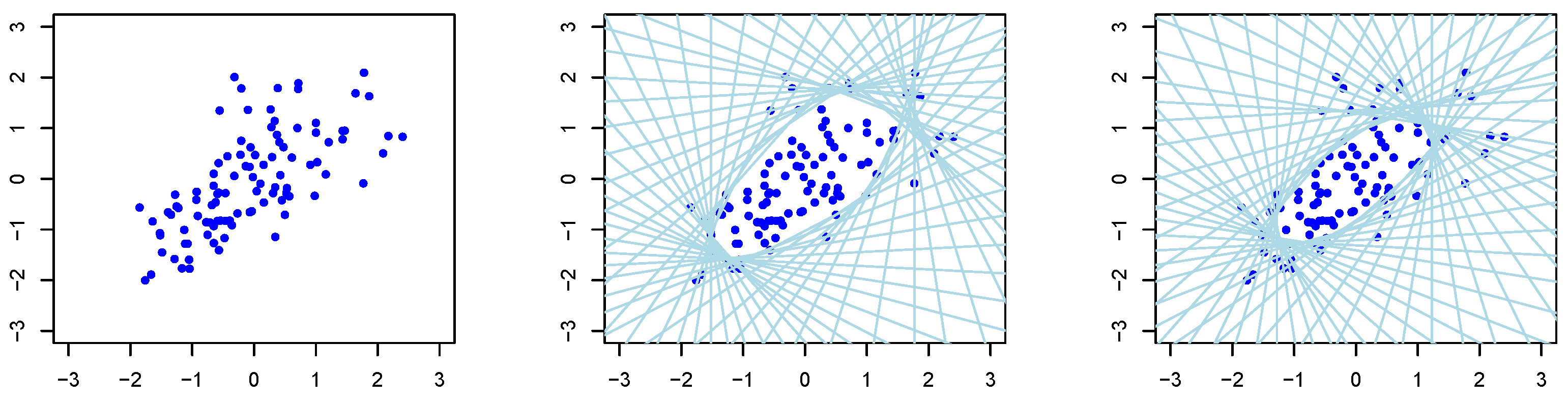
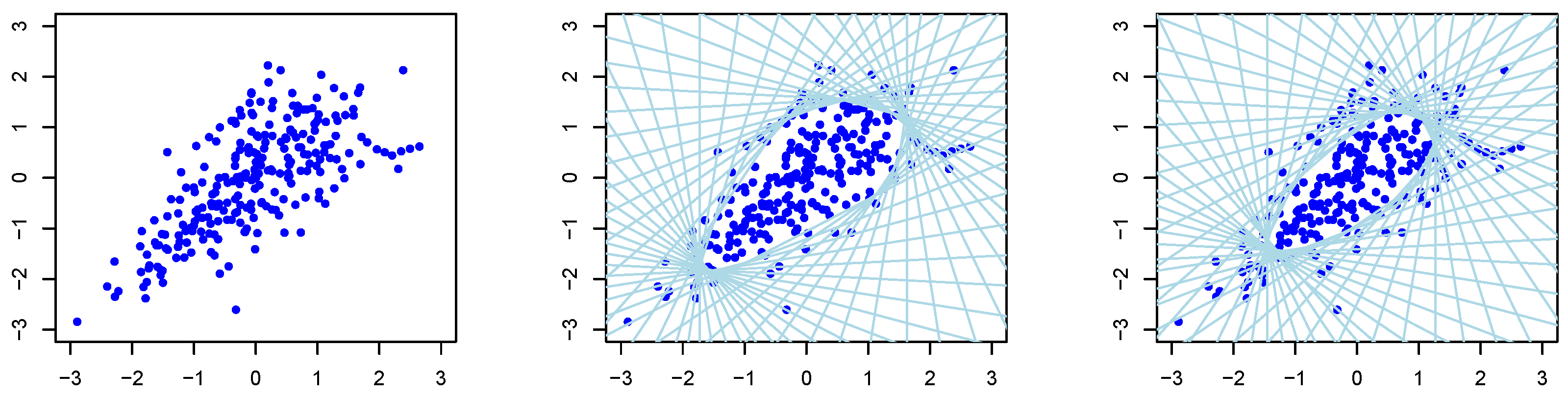
The middle and left panels of Figure 1 and Figure 2 show a set of approximated halfspaces as well as the resulting $\alpha$-depth regions being the open space in the middle within all the halfspaces. The TDC is given as the border of this open space.

4. ABC Based on Tukey Depth Statistics

As pointed out in the introduction, TDCs are highly flexible and able to capture almost any property of a multivariate sample. Therefore, they are appealing to use as statistics in ABC to efficiently compare the level of difference in properties between the observations and the generated samples from the model.

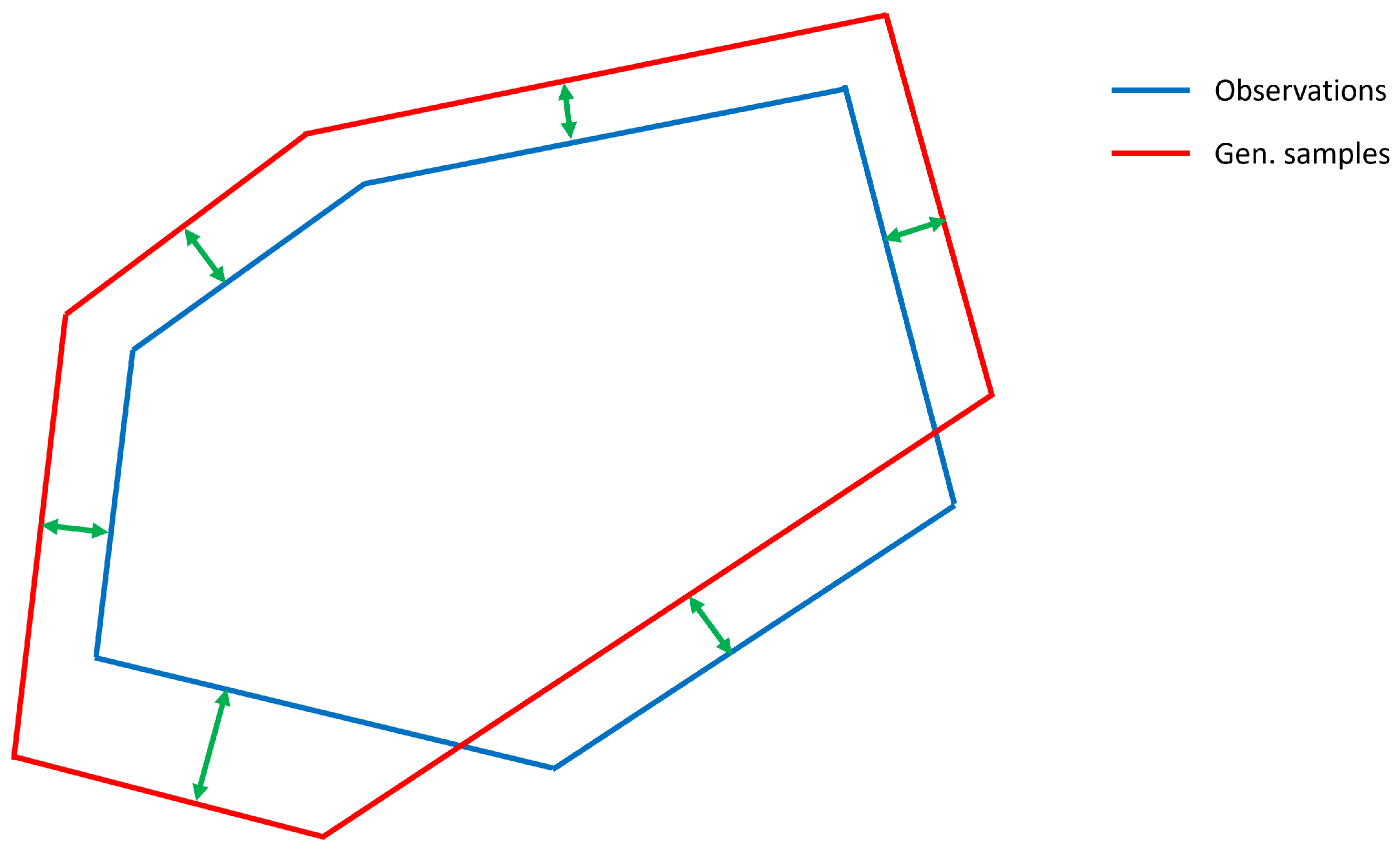
An open question is how to compare the difference between the Tukey depth contours of the observations and the generated samples. One natural and powerful metric is Intersection over Union (IoU) [42], which is highly popular for comparing segments in image analysis. However, in this paper we use the computationally simpler alternative of computing the difference between the contours in the directions defined by $u_i,i\in 1,\dots ,n_u$. This is illustrated in Figure 3. The red and blue lines show an illustration of a TDC computed from a set of observations and generated samples for $n_u=6$. The regions within the lines are the $\alpha$-depth regions. The green arrows show the difference between the TDCs along the directions $u_i,i\in 1,\dots ,6$.

As a comparison, IoU is computed by dividing the area of the intersection of the two Tukey depth regions by the area of the union of the two regions.

Further, it is possible to compare the TDCs of the observations and generated samples for multiple values of $\alpha$, i.e., multiple TDCs. The resulting ABC rejection sampling algorithm using TDCs as statistics is shown in Algorithm 2.

Algorithm 2 ABC rejection sampling using TDC statistics.

Input: N // Number of iteration $\mathbf{x}=x_1,x_2,\dots ,x_n$ // Dataset ${\alpha }_1,\dots ,{\alpha }_k$ // $\alpha$’s used to define TDCs $ϵ$ // Threshold $\widehat{\theta }=⌀$ // The set of accepted approximate posterior samples Method: 1: for  $n\in 1,2,\dots ,N$  do 2:    $\tilde{\theta }\leftarrow P\left(\theta \right)$ // Sample from prior distribution 3:    $\tilde{\mathbf{x}}={\tilde{x}}_1,\dots ,{\tilde{x}}_n\leftarrow P\left(x\right|\tilde{\theta })$ // Sample from generative model 4:    $\rho \leftarrow {\sum }_{j=1}^k{\sum }_{i=1}^{n_u}\left|{\widehat{Q}}_i({\alpha }_j,\mathbf{X})-{\widehat{Q}}_i({\alpha }_j,\tilde{\mathbf{X}})\right|$ 5:    if $\rho <ϵ$ then 6:      $\widehat{\theta }\leftarrow \widehat{\theta }\cup \tilde{\theta }$ // Add the accepted proposal $\tilde{\theta }$ to the set of accepted samples $\widehat{\theta }$ 7:    end if 8: end for 9: return  $\widehat{\theta }$

Specifically, line 4 in the algorithm measures the difference between a TDC computed from the observations and a TDC computed from generated samples.

5. Synthetic Experiments

As mentioned in the introduction, the mean vector and covariance matrix are the most commonly used statistics in likelihood free estimation such as ABC. In this section we demonstrate how the use of Tukey depth statistics results in more flexible and effective ABC parameter estimation compared to using the mean vector and covariance matrix.

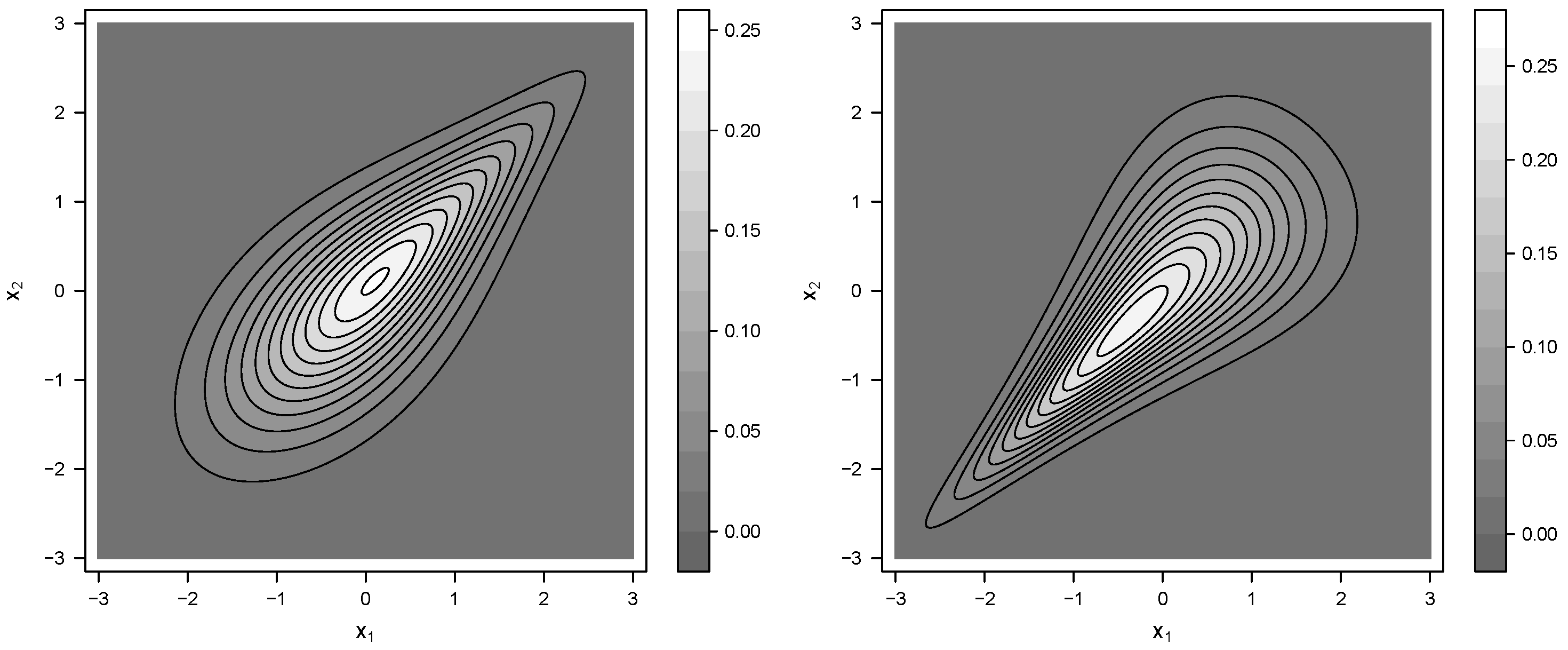
We consider the problem of estimating the mixture parameter $\theta \in [0,1]$ of the mixture distribution

$$P\left(x\right|\theta )=\theta f(x)+(1-\theta \left)g\right(x),-\infty <x<\infty .$$

(9)

The distribution $f\left(x\right)$ refers to a bivariate distribution with standard normal marginal distributions and dependency given by the Gumbel copula with $\gamma =2$. The distribution $g\left(x\right)$ is equal to $f\left(x\right)$ except that the dependency is by the Clayton copula with $\gamma =2.13$. A short introduction to copulas and details on the Gumbel and Clayton copulas are given in Appendix A. Figure 4 shows contour plots of the distributions $f\left(x\right)$ and $g\left(x\right)$.

Even though the two distributions look quite different, they have the same marginal expectations, variances and correlations.

In order to estimate the mixture parameter $\theta$ using ABC, it is essential that we can generate samples from the mixture distribution $P\left(x\right|\theta )$, as given in Equation (9). The mixture parameter $\theta$ controls the portion of samples that should be generated from $f\left(x\right)$ and $g\left(x\right)$. Therefore, to generate a sample, first, a random number $\eta$ is drawn from the uniform distribution on [0, 1]. If $\eta <\theta$, the sample is drawn from $f\left(x\right)$ else, the sample is drawn from $g\left(x\right)$.

Since the mean, variance, and correlation are identical for $f\left(x\right)$ and $g\left(x\right)$, it is naturally impossible to estimate the portions of the samples that were drawn from each of the two distributions using these statistics in likelihood-free estimation. In terms of these statistics, the distributions $f\left(x\right)$ and $g\left(x\right)$ are identical. However, we will demonstrate that, rather than using TDCs as statistics, the mixture parameter can be estimated.

We used the uniform distribution on $[0,1]$ as a prior distribution for $\theta$. Given the observation $\mathbf{x}=(x_1,\dots ,x_n)$, the resulting posterior distribution becomes as given by Equation (1).

Let $\widehat{\theta }={\widehat{\theta }}_1,\dots ,{\widehat{\theta }}_m$ represent samples from an approximation to the posterior distribution using ABC. To evaluate the quality of the approximation, we suggest comparing true posterior probabilities

$$P_J=P(\theta \in J)={\int }_{J}P\left(\theta \right|\mathbf{x})\mathrm{d}x$$

(10)

with approximations based on the samples

$${\widehat{P}}_J=\widehat{P}(\theta \in J)=\frac{1}{m}\sum _{i=1}^{m}I\left({\widehat{\theta }}_i\in J\right),$$

(11)

where J refers to some sub-interval of $[0,1]$ and $I(·)$ the indicator function. In the experiments, we used ten different intervals J.

5.1. Experiment

We started by generating 30 synthetic datasets of size $n=100$ and size $n=250$ from $P\left(x\right|\theta )$ with $\theta =0.3$. The left panel of Figure 1 and Figure 2 shows an example of such a dataset for $n=100$ and $n=250$, respectively. The middle and right panels show the halfspaces and resulting TDC as the inner border of all the halfspaces for $\alpha =0.05$ and $0.1$, respectively. Since $\theta =0.3$, on average 30% and 70% of the samples were generated from $f\left(x\right)$ and $g\left(x\right)$, respectively. Since most of the samples are generated from $g\left(x\right)$, the data are slightly spread in the upper right part according to the property of $g\left(x\right)$, as shown in Figure 4.

For each of the synthetic datasets, we used the ABC rejection algorithm to estimate the posterior probabilities in Equation (10). As discussed above, the quality of the approximation to the true posterior distribution depends on the statistics used in the ABC algorithm. Therefore, we compared the following four sets of statistics.

• TDC with $\alpha =0.05$
• TDC with $\alpha =0.4$
• Multiple TDCs for $\alpha =0.05,0.1,0.2$ and $0.4$
• Common statistics (mean and covariance matrix)

For each simulation of the ABC rejection algorithm (Algorithms 1 and 2), a total of $N={10}^5$ iterations were run, and the 1% of the $\tilde{\theta }$ samples with the smallest distance, $\rho$, were accepted and added to $\widehat{\theta }$ (code line 5 in Algorithm 1 and code line 6 in Algorithm 2). All experiments, including the generation of the synthetic datasets, were repeated five times to remove any noticeable Monte Carlo error in the results. In all experiments, $n_u=10$ directional vectors were used, but new vectors were generated for each independent run to ensure that the results did not depend on any specific choices of directional vectors.

The performance for a set of summary statistics in the ABC algorithm to approximate the true posterior probabilities was measured by the average mean absolute errors (AMAEs)

$$\mathrm{AMAE}=\frac{1}{30·5}\sum _{i=1}^{30}\sum _{k=1}^5|{\widehat{P}}_{J,i,k}-P_{J,i}|,$$

(12)

where the sums go over the 30 datasets and five Monte Carlo repetitions. $P_{J,i}$ and ${\widehat{P}}_{J,i,k}$ refer to the true posterior probability and its k-th Monte Carlo estimate, respectively.

The computations were run using the EasyABC package in R [43]. More specifically we used EasyABC to run the rejection algorithm.

5.2. Results

Table 1. Performance of four summary statistics choices via AMAE when $n=100$.

Interval	TDC $(\mathit{\alpha }=0.05)$	TDC $(\mathit{\alpha }=0.4)$	Multiple TDCs	Common Stats
$(0.2,0.8)$	0.185	0.192	0.188	0.225
$(0.3,0.7)$	0.208	0.205	0.211	0.237
$(0.4,0.6)$	0.140	0.132	0.133	0.140
$(0.1,0.3)$	0.155	0.132	0.143	0.206
$(0.3,0.5)$	0.159	0.153	0.160	0.185
$(0.5,0.7)$	0.102	0.098	0.106	0.117
$(0.7,0.9)$	0.100	0.096	0.107	0.181
$(0.1,0.4)$	0.183	0.181	0.185	0.282
$(0.6,0.9)$	0.146	0.149	0.147	0.237
$(0.4,0.5)$	0.082	0.080	0.081	0.091
Average	0.146	0.142	0.146	0.190

and

Table 2. Performance of four summary statistics choices via AMAE when $n=250$.

Interval	TDC $(\mathit{\alpha }=0.05)$	TDC $(\mathit{\alpha }=0.4)$	Multiple TDCs	Common Stats
$(0.2,0.8)$	0.241	0.203	0.201	0.270
$(0.3,0.7)$	0.225	0.212	0.219	0.266
$(0.4,0.6)$	0.152	0.157	0.166	0.181
$(0.1,0.3)$	0.211	0.218	0.207	0.264
$(0.3,0.5)$	0.226	0.218	0.215	0.280
$(0.5,0.7)$	0.109	0.113	0.134	0.162
$(0.7,0.9)$	0.054	0.048	0.063	0.177
$(0.1,0.4)$	0.265	0.270	0.286	0.422
$(0.6,0.9)$	0.106	0.101	0.128	0.262
$(0.4,0.5)$	0.108	0.104	0.108	0.120
Average	0.170	0.164	0.173	0.240

show AMAE for each of the ten intervals and, on average, for the four different sets of statistics for datasets of sizes $n=100$ and $n=250$, respectively, rounded to three decimal places. We see for both cases that using TDC statistics clearly performs better than using the common statistics in estimating the true posterior probabilities of the mixture parameter. This was also confirmed by statistical tests. We further see that the three sets of statistics based on TDC perform about equally well, and statistical tests did not reveal any difference in performance between them. We see that AMAE is higher for some intervals for $n=250$ compared $n=100$, and it might be surprising that the AMAE increases with dataset size. The explanation is that with increasing dataset size, the posterior distribution will be sharper around the true parameter values, and therefore, the probability for some of the intervals (or part of them) becomes very small, making the estimation of the true posterior probabilities more challenging.

6. Real-Life Experiments

The CPU (or GPU) processor of a computer system will over time typically receive tasks of varying sizes, and the rate of received tasks typically vary with time. For example, that more tasks will be received during office hours compared to other times of the day.

In this section, we consider the problem of estimating the statistical properties of these request patterns to the CPU processor using the computer system’s historical CPU usage. The statistical distributions characterising the request patterns are formulated below. It is usually only possible to observe the average CPU usage in disjoint time intervals of the day (e.g., ten-minute intervals), and it turns out that it is impossible to evaluate the likelihood function for the underlying request patterns [44]. Likelihood-free estimation is, therefore, the best option to estimate the underlying request patterns.

We will demonstrate how ABC with TDC statistics can be used to estimate unknown request patterns.

6.1. Data Generating Model

6.1.1. Notation

Assume that our CPU consumption data are collected on D working days. Since the data are only observed discretely over each day, we first let the time be measured in days and divide each day into T disjoint sub-intervals ${\delta }_1,\dots ,{\delta }_T$ which are of the same length and separated by $(T+1)$ time points

$$0={\tau }_0<{\tau }_1<\cdots <{\tau }_T=1.$$

Let ${\overline{y}}_{dt}$ denote the average CPU consumption in time interval ${\delta }_t$ on day d and let $y_d\left(\tau \right)$ denote the exact CPU consumption at some time $\tau \in [0,1]$ on day d. Recall from the discussions above that $y_d\left(\tau \right)$ is unobservable.

Furthermore, assuming that there are $N_d$ requests to the CPU processor on the day d, we denote the arrival times for each of these requests as $a_{d1},\dots ,a_{d{N}_d}$, and denote the size (CPU processing time) of these requests as $s_{d1},\dots ,s_{d{N}_d}$, respectively. We assume that an infinite number of CPU cores are available (thus no queueing of tasks), and therefore the departure times for the requests are $h_{dn}=a_{dn}+s_{dn},n\in 1,\dots ,N_d$.

6.1.2. Statistical Queuing Model

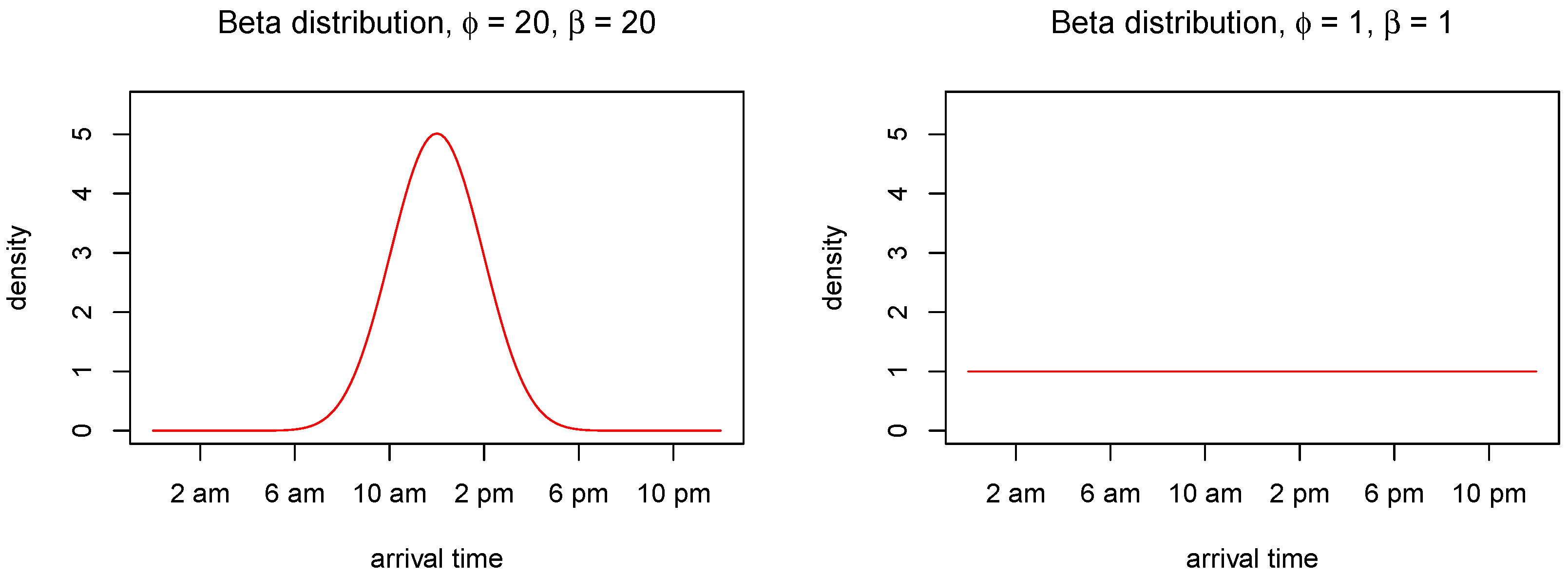
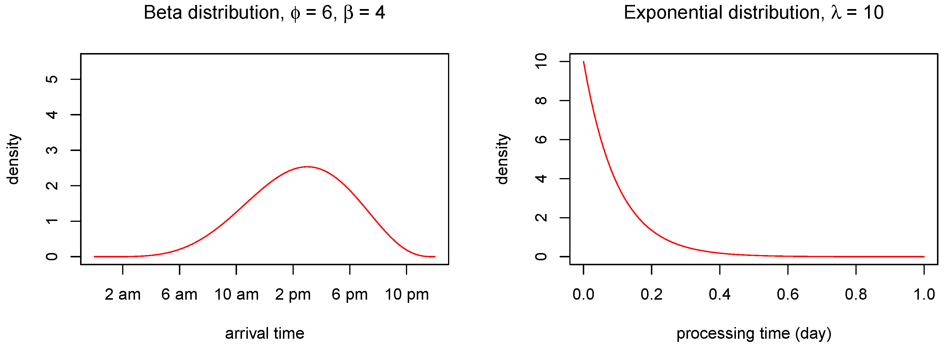
We assume that the arrival times are independent outcomes from a Beta distribution

$$a_{d1},\dots ,a_{d{N}_d}\stackrel{\mathrm{i}.\mathrm{i}.\mathrm{d}.}{˜}\mathrm{Beta}(\varphi ,\beta ),d=1,\dots ,D.$$

(13)

Different choices of the shape parameters $\alpha$ and $\beta$ yield different circumstances. For instance, if both of the shape parameters are high, e.g., $\varphi =\beta =20$, almost all arrivals (CPU requests) will take place within a short time period in the middle of the day (e.g., office hours). On the other hand, if $\varphi =\beta =1$, the arrivals will be uniformly distributed throughout the day. Figure 5 shows the beta distribution under these two parametric choices. For more details about the Beta distribution, see e.g., [14].

Further, we assume that the sizes (CPU processing time) for each request are independent outcomes from an exponential distribution with rate $\lambda$

$$s_{d1},\dots ,s_{d{N}_d}\stackrel{\mathrm{i}.\mathrm{i}.\mathrm{d}.}{˜}\mathrm{Exp}\left(\lambda \right),d=1,\dots ,D.$$

(14)

The expected CPU processing time is therefore $1/\lambda$.

Consequently, the current CPU consumption at some time $\tau \in [0,1]$ on day d is given by the requested tasks that are not yet finished.

$$y_d\left(\tau \right)=\sum _{n=1}^{N_d}I(a_{dn}<\tau <h_{dn}).$$

(15)

It follows that the average CPU consumption for a given time interval is

$${\overline{y}}_{dt}=\frac{1}{{\tau }_t-{\tau }_{t-1}}{\int }_{{\tau }_{t-1}}^{{\tau }_t}{y}_d\left(\tau \right)d\tau .$$

(16)

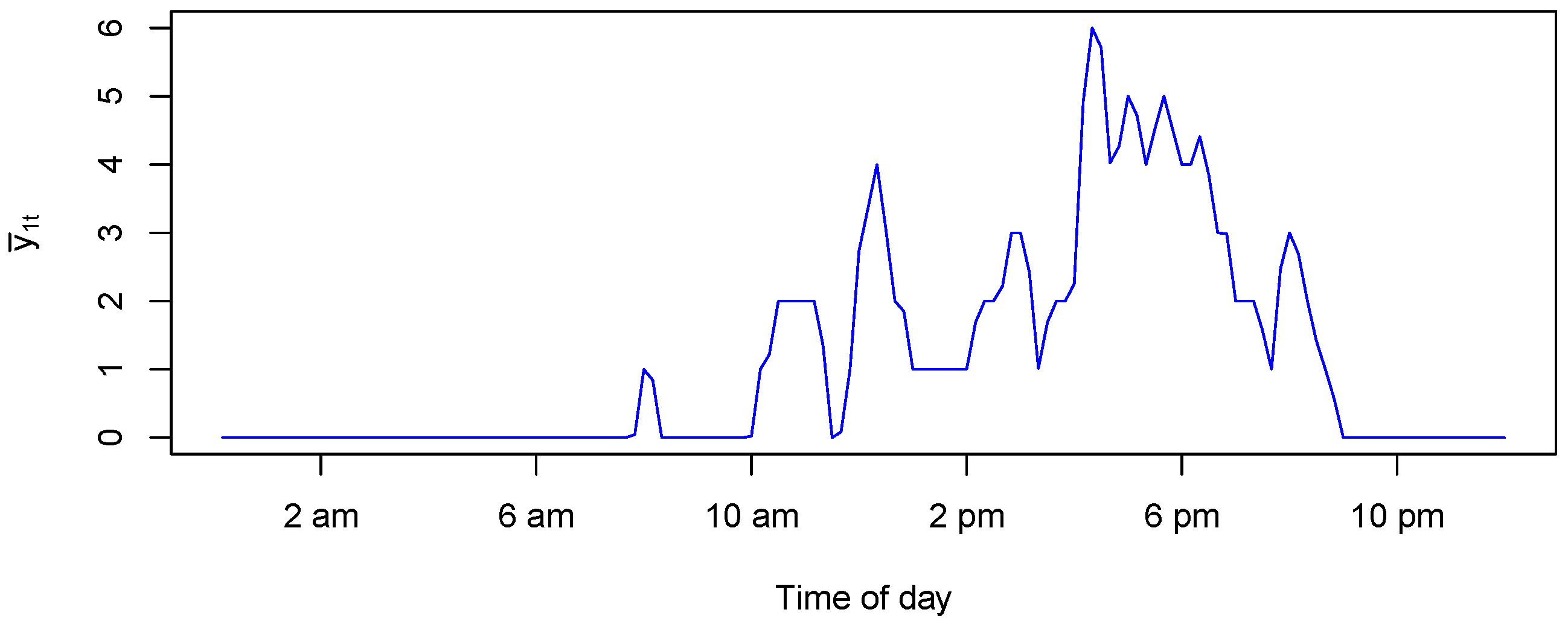
Figure 6 shows an example of a generated ${\overline{y}}_{dt}$ for one day using $\varphi =6$, $\beta =4$, $\lambda =10$, $T=144$ and $N_d=20$.

The resulting distributions for arrival and processing times are shown in Figure 7. We observe that the CPU usage is zero during the first part of the day since the probability of receiving requests is very small, as shown in the left panel of Figure 7. As soon as the requests are received, the CPU load increases. When the rate of request decreases, the CPU usage also gradually decreases.

6.2. Experiments and Results

Given observations ${\overline{y}}_{dt},d=1,\dots ,D,t=1,\dots ,T$, we consider the problem of estimating the parameters $\varphi$, $\beta$ and $\lambda$ of the beta and exponential distributions formulated above. In [44], Hammer et al. presented the resulting likelihood functions and explained why it is not possible to compute them. We, therefore, resort to ABC to estimate the parameters, and below we explain the summary statistics used.

For each day d, we suggest the following three statistics

$$S_{1d}:=\frac{1}{T}\sum _{t=1}^T{\overline{y}}_{dt},$$

(17)

$$S_{2d}:=\sum _{t=1}^{T}t·\left(\frac{{\overline{y}}_{dt}}{{\sum }_{t=1}^T{\overline{y}}_{dt}}\right),$$

(18)

$$S_{3d}:=\sum _{t=1}^T{t}^2\left(\frac{{\overline{y}}_{dt}}{{\sum }_{t=1}^T{\overline{y}}_{dt}}\right)-{\left[\sum _{t=1}^{T}t·\left(\frac{{\overline{y}}_{dt}}{{\sum }_{t=1}^T{\overline{y}}_{dt}}\right)\right]}^2.$$

(19)

The reasons for these choices of statistics are as follows. $S_{1d}$ is the mean CPU consumption on day d, and is directly related to the expected sizes of the tasks, $\lambda$, since the number of tasks per day is assumed to be known. Next, $S_{2d}$ is the mean time of the day when tasks are received, that is, are the tasks mainly received early on the day or later in the day. This is directly related to the expectation of the Beta distribution in Equation (13). Finally, $S_{3d}$ is the variance in when the tasks are received, i.e., whether they are all received in a small time interval or more evenly spread throughout the day. This statistic is directly related to the variance of the Beta distribution. In summary, these three statistics should be able to capture the main properties of the data to efficiently estimate the three unknown parameters $\varphi$, $\beta$, and $\lambda$.

Computing the three statistics for D days results in a total of $3D$ statistics.

$${\mathbf{S}}_1:=(S_{11},\dots ,S_{1D}),{\mathbf{S}}_2:=(S_{21},\dots ,S_{2D}),{\mathbf{S}}_3:=(S_{31},\dots ,S_{3D}).$$

(20)

Recall from the last passage of Section 4 that the Tukey depth contours are especially useful to reduce the high dimensionality of the set of summary statistics. Therefore, to sufficiently extract the main properties of the $3D$-dimensional distribution of $({\mathbf{S}}_1,{\mathbf{S}}_2,{\mathbf{S}}_3)$, we estimate the Tukey depth contours of the distribution of the statistics over the D days. In other words, we use $({\mathbf{S}}_1,{\mathbf{S}}_2,{\mathbf{S}}_3)$ as $\mathbf{X}$ in the method in Section 4. As an alternative, we could simply compute the average of the statistics over all the $D=40$ each day, but given that the statistics are not sufficient [4] for the unknown parameters, computing the Tukey depth contours will be able to provide us with more information, which again will improve the estimation of the unknown parameters.

We assumed that the CPU usage times were observed for $D=40$ days and that the observations were the average CPU usage in $T=144$ disjoint time intervals per day, i.e., 10 min intervals. Finally, we assumed that the number of tasks per day was $N_d=20$ for $d=1,\dots ,40$.

In addition, we assumed that the true values of the unknown parameters were $\varphi =6$ and $\beta =4$ so that almost all arrivals (CPU requests) will take place from 5 a.m. to 10 p.m., as shown in the left panel of Figure 7. The processing time for each request was assumed to follow the exponential distribution with rate $\lambda =10$, as shown in the right panel of Figure 7. These parameter values were used to generate a synthetic dataset, and the aim was to use the ABC rejection algorithm with TDC statistics, as described above, to estimate the parameter values used to generate the synthetic dataset.

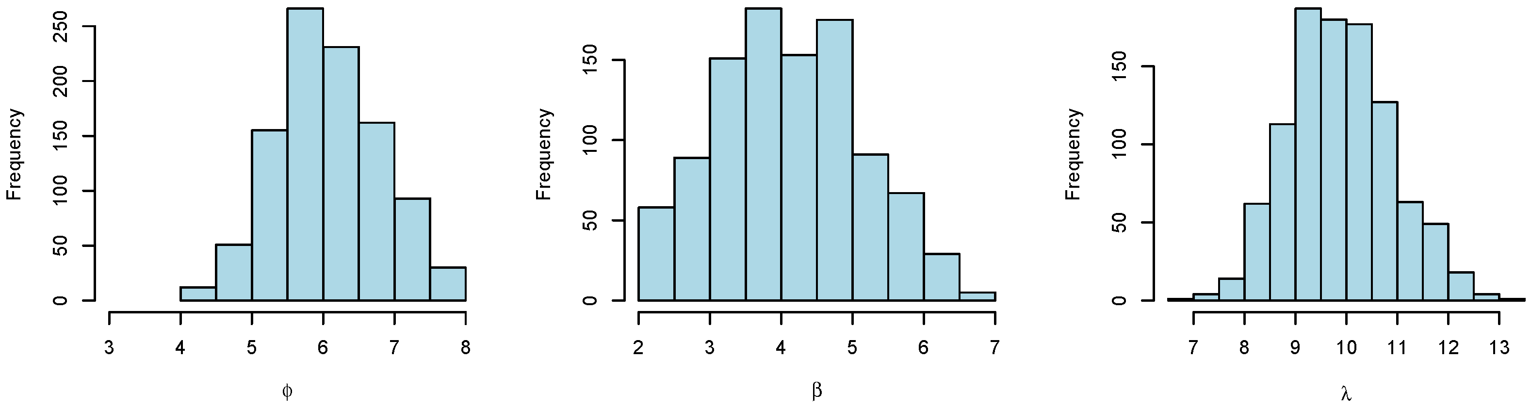
We used uniform prior distributions for the three parameters $\varphi$, $\beta$ and $\lambda$ on the supports $(3,8)$, $(2,7)$, and $(3,40)$, respectively. We used $n_u=10$ directional vectors to compute the TDCs. We used TDC statistics for $\alpha =0.05$. In the ABC rejection algorithm, we generated ${10}^5$ samples and kept the 1% of samples with the smallest distance $\rho$ in Algorithm 2.

Figure 8 shows histograms of the resulting posterior samples of $\varphi$, $\beta$, and $\lambda$.

We see that we are able to estimate the unknown parameters and that the true values of the parameters (which were used to generate the synthetic data) are centrally positioned in each histogram. We further see that the histograms are quite wide, demonstrating that the problem of estimating the underlying request patterns from observed CPU usage is a challenging task.

7. Closing Remarks

A fundamental challenge in likelihood free estimation is how to select statistics that are able to capture the properties of the data that are important for efficient estimation of the unknown model parameter values. The optimal choice is to choose the sufficient statistics for the unknown parameters, but they are rarely known for generative models.

In this paper, we have developed a framework for efficiently using TDC statistics in likelihood-free estimation. To the best of our knowledge, TDCs have not been used for likelihood-free estimation before. TDCs are highly flexible and able to capture almost any properties of the data. The experiments show that the TDC statistics are more efficient than the more commonly used statistics mean vector, variances and correlations in estimating the mixture parameter of a mixture distribution. TDCs are further used to estimate request patterns to a computer system.

A potential improvement of the suggested method is to use a better metric for comparing the TDCs for the dataset and generated sample, for example, using IoU as suggested in Section 4. Another interesting direction for future work is to use TDCs in combination with other likelihood-free estimation techniques such as ABC MCMC, ABC Sequential Monte Carlo or auxiliary model techniques [7].

References

- Achiam, J.; Adler, S.; Agarwal, S.; Ahmad, L.; Akkaya, I.; Aleman, F.L.; Almeida, D.; Altenschmidt, J.; Altman, S.; Anadkat, S.; et al. GPT-4 Technical Report. arXiv 2023, arXiv:cs.CL/2303.08774. [Google Scholar]
- Ho, J.; Jain, A.; Abbeel, P. Denoising diffusion probabilistic models. Adv. Neural Inf. Process. Syst. 2020, 33, 6840–6851. [Google Scholar]
- Aggarwal, A.; Mittal, M.; Battineni, G. Generative adversarial network: An overview of theory and applications. Int. J. Inf. Manag. Data Insights 2021, 1, 100004. [Google Scholar] [CrossRef]
- Casella, G.; Berger, R.L. Statistical Inference; Cengage Learning: Boston, MA, USA, 2021. [Google Scholar]
- Lintusaari, J.; Vuollekoski, H.; Kangasraasio, A.; Skytén, K.; Jarvenpaa, M.; Marttinen, P.; Gutmann, M.U.; Vehtari, A.; Corander, J.; Kaski, S. Elfi: Engine for likelihood-free inference. J. Mach. Learn. Res. 2018, 19, 1–7. [Google Scholar]
- Goodfellow, I.; Pouget-Abadie, J.; Mirza, M.; Xu, B.; Warde-Farley, D.; Ozair, S.; Courville, A.; Bengio, Y. Generative adversarial networks. Commun. ACM 2020, 63, 139–144. [Google Scholar] [CrossRef]
- Beaumont, M.A. Approximate bayesian computation. Annu. Rev. Stat. Its Appl. 2019, 6, 379–403. [Google Scholar] [CrossRef]
- Kong, L.; Mizera, I. Quantile tomography: Using quantiles with multivariate data. Stat. Sin. 2012, 22, 1589–1610. [Google Scholar] [CrossRef]
- Hammer, H.L.; Yazidi, A.; Rue, H. Estimating Tukey depth using incremental quantile estimators. Pattern Recognit. 2022, 122, 108339. [Google Scholar] [CrossRef]
- Tukey, J.W. Mathematics and the Picturing of Data. In Proceedings of the International Congress of Mathematicians, Vancouver, BC, Canada, 21–29 August 1975. [Google Scholar]
- Mahalanobis, P.C. On the generalized distance in statistics. In Proceedings of the National Institute of Sciences of India; National Institute of Sciences of India: Prayagraj, India, 1936. [Google Scholar]
- Barnett, V. The ordering of multivariate data. J. R. Stat. Soc. Ser. A 1976, 139, 318. [Google Scholar] [CrossRef]
- Oja, H. Descriptive statistics for multivariate distributions. Stat. Probab. Lett. 1983, 1, 327–332. [Google Scholar] [CrossRef]
- Liu, R.Y. On a Notion of Data Depth Based on Random Simplices. Ann. Stat. 1990, 18, 405–414. [Google Scholar] [CrossRef]
- Koshevoy, G.; Mosler, K. Zonoid trimming for multivariate distributions. Ann. Stat. 1997, 25, 1998–2017. [Google Scholar] [CrossRef]
- Vardi, Y.; Zhang, C.H. The multivariate L1-median and associated data depth. Proc. Natl. Acad. Sci. USA 2000, 97, 1423–1426. [Google Scholar] [CrossRef] [PubMed]
- Rousseeuw, P.J.; Ruts, I. Algorithm AS 307: Bivariate Location Depth. J. R. Stat. Soc. Ser. C 1996, 45, 516. [Google Scholar] [CrossRef]
- Peter, J.; Rousseeuw, I.R.; Tukey, J.W. The Bagplot: A Bivariate Boxplot. Am. Stat. 1999, 53, 382–387. [Google Scholar]
- Liu, R.Y.; Parelius, J.M.; Singh, K. Multivariate analysis by data depth: Descriptive statistics, graphics and inference, (with discussion and a rejoinder by Liu and Singh). Ann. Stat. 1999, 27, 783–858. [Google Scholar] [CrossRef]
- Buttarazzi, D.; Pandolfo, G.; Porzio, G.C. A boxplot for circular data. Biometrics 2018, 74, 1492–1501. [Google Scholar] [CrossRef]
- Liu, R.Y.; Singh, K. A quality index based on data depth and multivariate rank tests. J. Am. Stat. Assoc. 1993, 88, 252. [Google Scholar]
- Becker, C.; Gather, U. The masking breakdown point of multivariate outlier identification rules. J. Am. Stat. Assoc. 1999, 94, 947. [Google Scholar] [CrossRef]
- Serfling, R. Depth functions in nonparametric multivariate inference. In DIMACS Series in Discrete Mathematics and Theoretical Computer Science; American Mathematical Society: Providence, RI, USA, 2006; pp. 1–16. [Google Scholar]
- Zhang, J. Some extensions of tukey’s depth function. J. Multivar. Anal. 2002, 82, 134–165. [Google Scholar] [CrossRef]
- Yeh, A.B.; Singh, K. Balanced confidence regions based on Tukey’s depth and the bootstrap. J. R. Stat. Soc. Ser. B (Methodol.) 1997, 59, 639–652. [Google Scholar] [CrossRef]
- Fraiman, R.; Liu, R.Y.; Meloche, J. Multivariate density estimation by probing depth. In Institute of Mathematical Statistics Lecture Notes—Monograph Series; Lecture Notes-Monograph Series; Institute of Mathematical Statistics: Hayward, CA, USA, 1997; pp. 415–430. [Google Scholar]
- Brown, B.M.; Hettmansperger, T.P. An affine invariant bivariate version of the sign test. J. R. Stat. Soc. 1989, 51, 117–125. [Google Scholar] [CrossRef]
- Hettmansperger, T.P.; Oja, H. Affine invariant multivariate multisample sign tests. J. R. Stat. Soc. Ser. B (Methodol.) 1994, 56, 235–249. [Google Scholar] [CrossRef]
- Li, J.; Liu, R.Y. New Nonparametric Tests of Multivariate Locations and Scales Using Data Depth. Stat. Sci. 2004, 19, 686–696. [Google Scholar] [CrossRef]
- Li, J.; Cuesta-Albertos, J.A.; Liu, R.Y. DD-classifier: Nonparametric classification procedure based on DD-plot. J. Am. Stat. Assoc. 2012, 107, 737–753. [Google Scholar] [CrossRef]
- Kim, S.; Mun, B.M.; Bae, S.J. Data depth based support vector machines for predicting corporate bankruptcy. Appl. Intell. 2018, 48, 791–804. [Google Scholar] [CrossRef]
- Hubert, M.; Rousseeuw, P.; Segaert, P. Multivariate and functional classification using depth and distance. Adv. Data Anal. Classif. 2017, 11, 445–466. [Google Scholar] [CrossRef]
- Jörnsten, R. Clustering and classification based on the L1 data depth. J. Multivar. Anal. 2004, 90, 67–89. [Google Scholar] [CrossRef]
- Kosiorowski, D.; Zawadzki, Z. DepthProc an R package for robust exploration of multidimensional economic phenomena. arXiv 2014, arXiv:1408.4542. [Google Scholar]
- Williams, B.; Toussaint, M.; Storkey, A.J. Modelling motion primitives and their timing in biologically executed movements. In Proceedings of the Advances in Neural Information Processing Systems, Vancouver, BC, Canada, 8–10 December 2008; pp. 1609–1616. [Google Scholar]
- Hubert, M.; Rousseeuw, P.J.; Segaert, P. Multivariate functional outlier detection. Stat. Methods Appl. 2015, 24, 177–202. [Google Scholar] [CrossRef]
- Cerdeira, J.O.; Monteiro-Henriques, T.; Martins, M.J.; Silva, P.C.; Alagador, D.; Franco, A.M.; Campagnolo, M.L.; Arsénio, P.; Aguiar, F.C.; Cabeza, M. Revisiting niche fundamentals with Tukey depth. Methods Ecol. Evol. 2018, 9, 2349–2361. [Google Scholar] [CrossRef]
- Chebana, F.; Ouarda, T.B. Depth-based multivariate descriptive statistics with hydrological applications. J. Geophys. Res. Atmos. 2011, 116, D10. [Google Scholar] [CrossRef]
- Marjoram, P.; Molitor, J.; Plagnol, V.; Tavaré, S. Markov chain Monte Carlo without likelihoods. Proc. Natl. Acad. Sci. USA 2003, 100, 15324–15328. [Google Scholar] [CrossRef] [PubMed]
- Beaumont, M.A.; Cornuet, J.M.; Marin, J.M.; Robert, C.P. Adaptive approximate Bayesian computation. Biometrika 2009, 96, 983–990. [Google Scholar] [CrossRef]
- Mosler, K. Depth statistics. In Robustness and Complex Data Structures; Springer: Berlin/Heidelberg, Germany, 2013; pp. 17–34. [Google Scholar]
- Minaee, S.; Boykov, Y.; Porikli, F.; Plaza, A.; Kehtarnavaz, N.; Terzopoulos, D. Image segmentation using deep learning: A survey. IEEE Trans. Pattern Anal. Mach. Intell. 2021, 44, 3523–3542. [Google Scholar] [CrossRef]
- Jabot, F.; Faure, T.; Dumoulin, N. EasyABC: Performing efficient approximate Bayesian computation sampling schemes using R. Methods Ecol. Evol. 2013, 4, 684–687. [Google Scholar] [CrossRef]
- Hammer, H.L.; Yazidi, A.; Bratterud, A.; Haugerud, H.; Feng, B. A Queue Model for Reliable Forecasting of Future CPU Consumption. Mob. Netw. Appl. 2017, 23, 840–853. [Google Scholar] [CrossRef]
- Hofert, M.; Kojadinovic, I.; Mächler, M.; Yan, J. Elements of Copula Modeling with R; Springer International Publishing: Berlin/Heidelberg, Germany, 2018. [Google Scholar]
- Joe, H. Dependence Modeling with Copulas; Chapman and Hall/CRC: Boca Raton, FL, USA, 2014. [Google Scholar]