1. Introduction
When we look at the world around us, we are implicitly engaging in a form of active data sampling (also known as active sensing or active inference [
1,
2,
3,
4,
5]). Despite the abundance of visual data available to us at any one moment, our visual systems are adapted to select (or foveate) only a small portion of these data. The advantage of this is that our brains can scale the processes that underwrite perceptual inference to large sensory datasets. All that is needed is an efficient means of sequentially selecting those data to best optimise our inferences about their causes [
6,
7].
This paper suggests that the same process of active sampling can be (and often is) used in situations in which there is a cost associated with collecting new data or analysing a very large dataset.
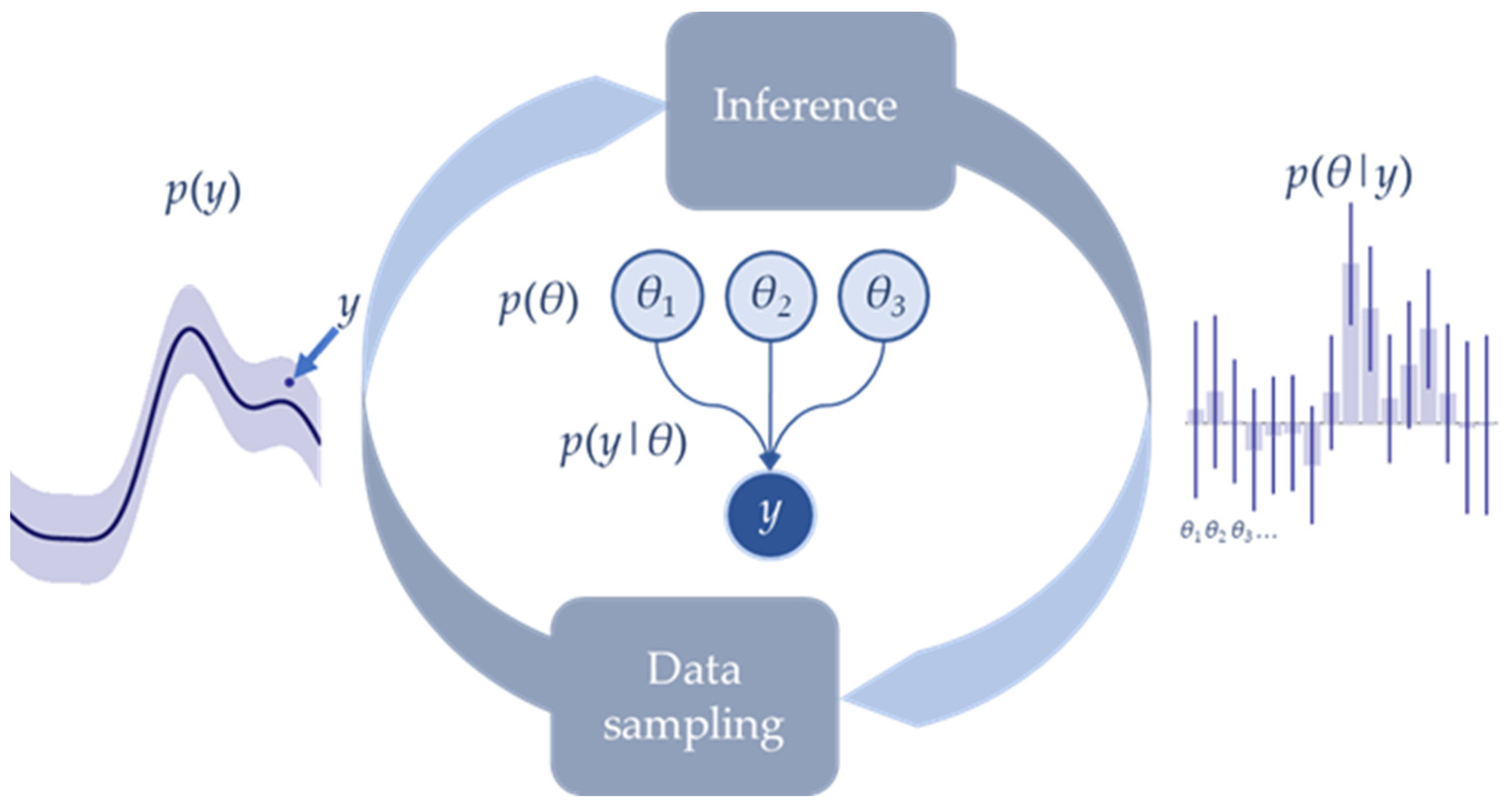
Figure 1 illustrates the basic idea, akin to perception–action cycles in biology [
8], of alternating between drawing inferences from the data we have available and selecting new data based on these inferences. This cycle is implicitly part of the scientific process, in which our pre-existing understanding is used to motivate experiments whose results update our understanding to motivate future experiments, and so on.
Within the schematic shown in
Figure 1, we highlight the key quantities in this cyclical process. They include the causes of data (which may include model parameters or hidden states) (
θ) and the data (
y). Bayesian inference involves taking our prior beliefs about causes
p(
θ), combining these with the likelihood (
p(
y|
θ)) of observed data, and arriving at a posterior belief (
p(
θ|
y)) as to the causes given the data. The priors and likelihoods together comprise what is known as a generative model, which can be represented in a number of ways, including as the Bayesian network shown in the centre of the graphic. Here, an arrow from one variable to another indicates a conditional probability distribution of the latter given the former.
Careful data selection is especially important when we consider the problems associated with very large datasets of the sort that are now ubiquitous in machine learning and artificial intelligence settings. Computations with such datasets can be costly in terms of the hardware and computing power required, and their energy consumption raises important sustainability questions [
9,
10,
11,
12]. Taking inspiration from the approach evinced by natural selection—that of sequentially selecting small amounts of sensory data—may help to alleviate the costs associated with big-data analysis.
To optimise data selection, we first need to identify an appropriate optimality criterion. In what follows, we base this upon the idea of expected information gain—a measure used in optimisation of experimental design [
13,
14], feature selection [
15], and accounts of biological information-seeking and curiosity-driven behaviour [
16,
17]. The idea behind this measure is that we form beliefs about hidden states or parameters in our model of how data are generated. Expected information gain is the degree to which we anticipate changing our beliefs under a given experimental design or data-sampling strategy. The implication is that optimisation of beliefs—and of data selection—work in tandem, as in
Figure 1, and that both depend upon our model of how data are generated.
In what follows, we consider the form this model, and therefore data-selection, might take in different settings, starting with abstract function-approximation and progressing to a more realistic example based upon the idea of an adaptive clinical trial. Before we move to these examples, we unpack the basic theory behind active data selection. We outline the basic principles behind Bayesian inference, the role of generative models, and the formulation of expected information gain. Our overall aim is to provide an intuitive overview of the principles that underwrite active data selection, and to illustrate this with some simple examples.
2. Bayesian Inference, Generative Models, and Expected Information Gain
Bayesian inference is the process of inverting a model of how data (
y) are generated to obtain two things [
18]. The first is the probability of observed data under our model—sometimes referred to as marginal likelihood. This is a ubiquitous measure of the evidence our data affords the hypothesis expressed in our model. Second is the probability of the random variables (
θ) in the model given our data—known as a posterior probability. These two things can be obtained by specifying the a priori plausible distributions of model variables and the likelihood of generating patterns of data given the values those variables might take. These prior and likelihood beliefs form our generative model. The relationship between the generative model and the associated marginal likelihood and posterior probability is given by Bayes’ theorem, which can be expressed as:
Equation (1) shows the generative model, its inversion, and the relationship between a model and its marginal likelihood. The second line shows that the marginal likelihood is obtained directly from the prior and likelihood beliefs simply by taking the expectation (or average) of the latter, assuming our
θ variables are distributed according to the prior (also known as marginalisation). This leaves only one unknown in the first line—the posterior—which can then be obtained from rearrangement of the other three terms. In practice,
θ may include many different parameters or hidden states, making exact computation impractical [
19]. While we will touch upon the topic of approximate inference briefly in one of the examples, this is of limited importance for the primary message of this paper. However, the question of how we deal with complex models with multiple parameters is important to address.
Bayesian networks, and related graphical notations, offer a visualisation of a generative model. They tell us which variables depend upon which other variables. This is useful in that it suggests efficient message passing schemes that may be used to perform an inference (see [
20,
21] for overviews). Such representations have broad applicability, ranging from clinical reasoning [
22] to environmental conservation [
23]. For our purposes, message passing in graphical models is useful in that it helps us to find the quantities required for computing expected information gain.
The information we gain on making an observation can be formalised as the change in our beliefs as a consequence of that observation. A change in probabilities of this sort is quantified using a KL-Divergence (also known as relative entropy)—the average difference between the log probabilities before and after that observation (i.e., between the prior and posterior of Equation (1)). The value this KL-Divergence takes, averaged over the data we would predict using our marginal likelihood, is our expected information gain [
14]:
In Equation (2), we have conditioned our model upon the variable π, which represents a choice we can make in selecting our data. The first line specifies expected information gain directly as the expectation of an information gain. The second line expresses information gain in terms of mutual information that quantifies the degree of conditional dependence between parameters and data. If the parameters were independent of data, the joint distribution would be equal to the product of their marginals, rendering the divergence zero. The third line provides a further interpretation in terms of the difference between two entropies. Essentially, the greater the predictive uncertainty the greater the potential information we can gain, but only if the conditional entropy is sufficiently small that there is a precise mapping from parameters to the data they cause.
The final line of Equation (2) re-expresses the penultimate line by explicitly separating the joint distributions into their constituent singleton (i.e., marginal) and conditional distributions. This gives a sense of a recursive structure, in which the key constituents of information gain are themselves built up of expectations of expectations (of expectations as the model becomes more complex). This provides us with a method for quantifying the information gain about parameters in graphical models. Such models are typically expressed using a series of nodes (or edges, in factor graphs) representing variables linked together by the factors of their associated probability distributions. Typically, causative variables are placed towards the top of the graph and measurable data at the bottom. Pairs of nodes are linked if there is a conditional dependence between them. In other words, two nodes are depicted as linked if there is a (conditional probability) factor of the model in which the variable represented by one of the two nodes is in the conditioning set (the ‘parent’) and the variable represented by the other node is the support (the ‘child’) of that factor.
Using the notation
pa( ) to represent parents of (i.e., the things something depends upon), and
ch( ) to represent children of (i.e., the things that depend upon it), we can express the expected information gain in Equation (2)—about a parameter
θi—in terms of messages (
μ) that are passed along the edges of the factor graph:
The Λ operator here is introduced to indicate either summation or integration—depending upon whether we are dealing with continuous or discrete variables—with respect to the variables indicated by the subscript. The recursive definitions of the messages (
μ) in Equation (3) are exactly the definitions that underwrite belief-propagation inference schemes, including the sum-product algorithm [
24]. Superscripts and subscripts on the messages indicate the node or variable from which the message comes, and to which it is sent, respectively. In what follows, we consider the nature of the requisite messages.
3. A Worked Example
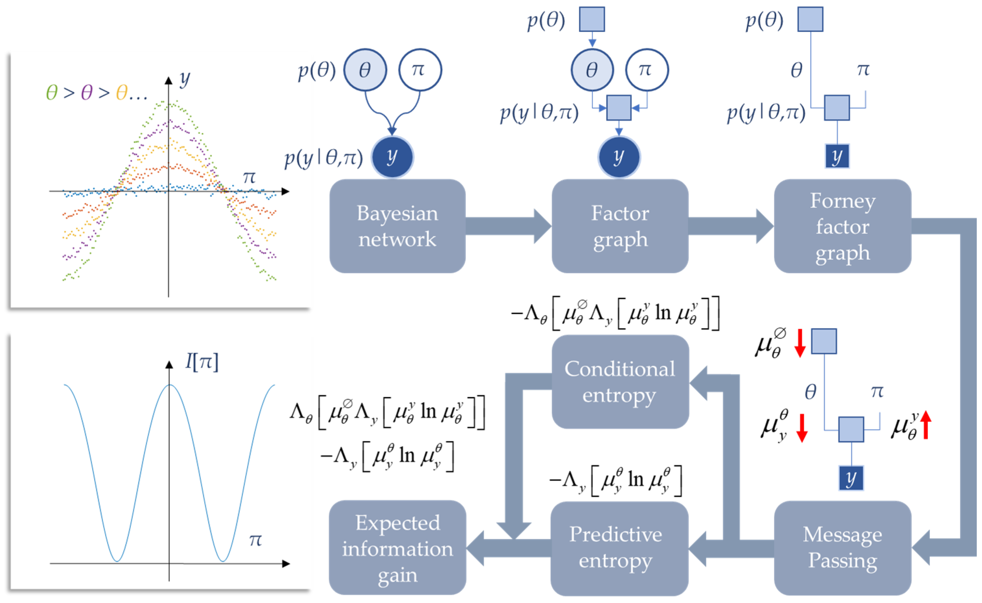
In
Figure 2, we illustrate a simple worked example based on Equation (3) using a Bayesian network of normally distributed variables. The network includes three nodes. These are: the choice (
π) we make about how to sample our data, the parameter (
θ) we seek information about, and our data (
y). The Bayesian network is first transformed into a factor graph—with explicit representation of factors of the joint probability distribution as boxes—and then to a (normal) Forney factor graph [
25] that omits the variable nodes (circles). The Forney factor graph formulation is perhaps the easiest to use when visualising the passing of messages along the edges of the graph. The messages can then be used to construct the two entropies we need to compute expected information gain.
The model in this toy example has the following factors:
In effect, this model amplifies or attenuates the amplitude of the predicted data depending upon a periodic function of our data-sampling policy,
π. The upper-left panel of
Figure 2 depicts the data sampled from this model for several possible values of
θ. Computing the relevant messages for the information gain, we have (omitting normalising constants for simplicity and using
to denote the empty set)
The directions of these messages are illustrated in the bottom-right panel of
Figure 2. We next substitute these into the first line of Equation (3) to find an expression for the information gain about the parameter
θ. Once all terms that are constant with respect to
π are eliminated, we are left with:
Equation (6) is a special case of the third row of
Table 1, which highlights analytical expressions for expected information gain for a few common model structures. This function is plotted in the lower-left panel of
Figure 2. As we might intuit, the most informative places to sample data align with those in which differences in
θ lead to large differences in the predicted data—i.e., in which our choice of π maximises the sensitivity with which
y depends upon
θ. Given that a periodic (cosine) function is used for the effect of how we chose to sample (π) the data (
y), there are multiple peaks which coincide with the peaks and troughs of the periodic function.
4. Function Approximation
We next turn to a generic supervised learning problem—that of trying to approximate some function based upon known inputs and the observable outcomes they (stochastically) cause. Our generative model for this is straightforward:
The matrix (Φ) comprises a set of concatenated row vectors (
ϕi). The columns of Φ are elements of some basis set. For the simulations that follow, these are Gaussian radial basis functions. In the MATLAB demo routines that accompany this paper, alternative basis sets (including cosine and polynomial) can be chosen. We can see this model as an approximation of an unknown function whose (discretised) input is the row index of Φ and whose output is the expected value of
y corresponding to that row:
Our choice of π is used to test alternative values of the input (
x) to see the output (
y) that the unknown function (
f) generates. Here, π indexes the discrete intervals of
x implicit in the columns of Φ.
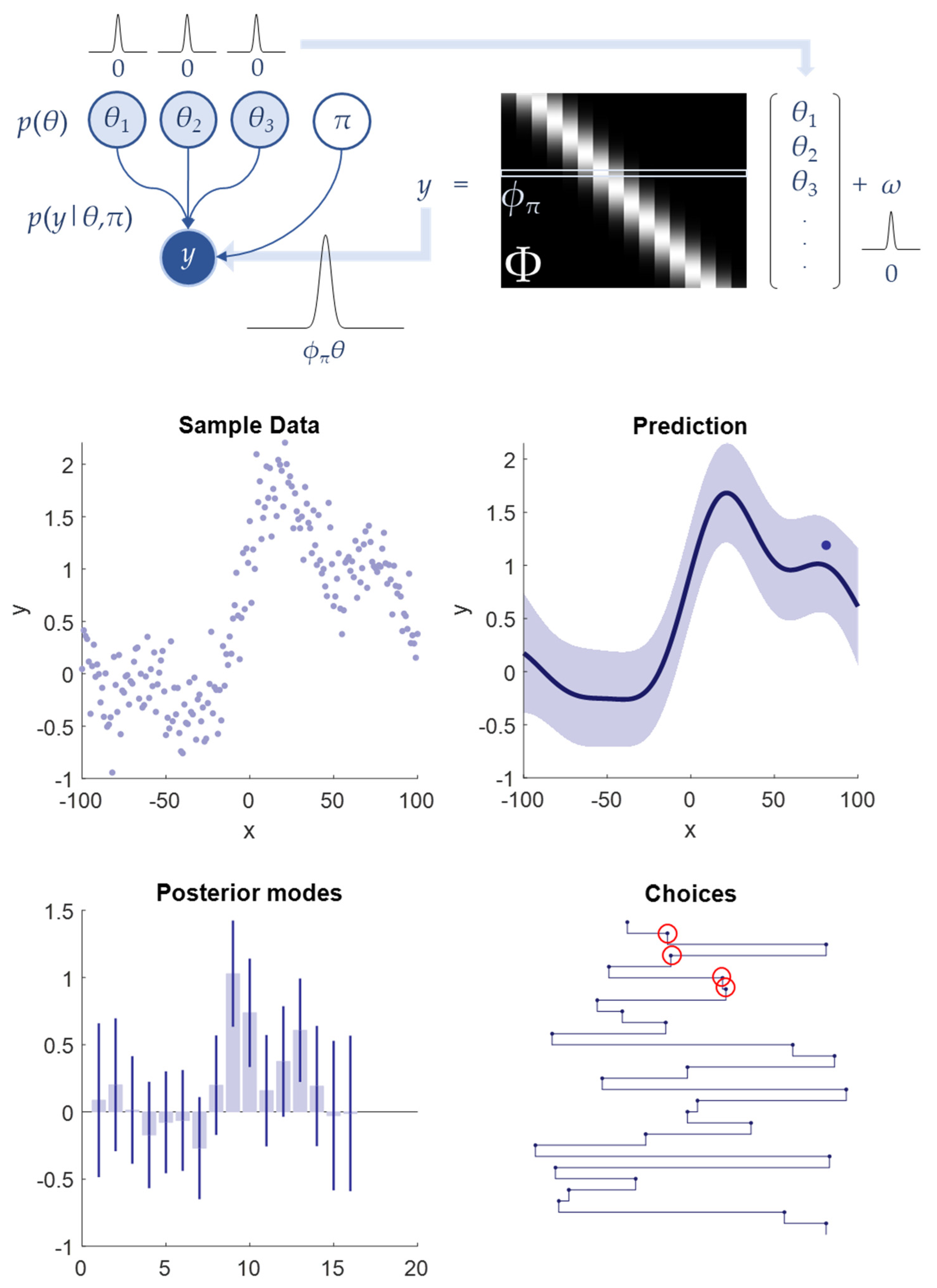
Figure 3 illustrates a depiction of this model as a Bayesian network and a visual representation of the data-generating process. In this simulation, we move beyond our worked example in
Figure 2 and consider multiple samples. In this setting, we replace our prior beliefs after each observation with our posterior beliefs, allowing a gradual refinement of our approximated function and the future choices on which this depends.
The posterior probability of the parameters following an input and the marginal probability of the data are:
The middle-right panel of
Figure 3 shows the predictive (marginal) probability distribution after 28 random choices for
π. The lower-left panel shows the posterior probabilities of the parameters. The specific choices are shown in the lower-right panel. Even with these random choices, the 28 samples provide a reasonably good approximation to the shape of the function, as can be seen comparing the middle-left (large number of samples drawn from the function) and right panels. However, a closer look at the choices made reveals some clear inefficiencies. For instance, choices 2 and 4 and choices 6 and 7 are very close to one another (circled in red). Intuitively, we would expect that for any (smooth) function, it will almost always be preferable to sample locations far away from one another, as some uncertainty will have been resolved by samples nearby.
This is where the information gain becomes relevant. Substituting Equation (7) into Equation (3), we have
Figure 4 shows the same set-up as in
Figure 3, but now samples are drawn from a distribution whose log is proportional to the information gain in Equation (10). During each iteration, a sample location is chosen from this distribution (a large proportionality constant makes this almost deterministic; i.e., the location with the highest information gain is almost always chosen). A datapoint is then sampled from the generative model under this choice. This is then used to update priors to posteriors using Equation (9). The process is then repeated up to 28 iterations.
Unlike the random sampling, it is not until late in the simulation that we revisit a previously sampled location. The implication is that we can achieve better inferences with the same, or perhaps even a smaller, number of samples when we select these samples in a smart way. This raises the question as to how many samples we should collect.
An answer to this question can be drawn from behavioural neuroscience and the so-called exploitation–exploration dilemma [
27,
28]. This deals with the situation in which certain parts of our environment may be particularly aversive or attractive—perhaps due to the presence of food or predators—but we do not know where these locations are to begin with. Initially, we must explore, seeking information about our environment, and then at some stage switch to exploiting the knowledge acquired, to ensure we occupy preferred locations. If all locations were equally preferrable, we could continue exploring forever, developing ever more precise beliefs about our world. The same is true when sampling data or performing experiments if there is no cost to performing this sampling. However, once we acknowledge the computational and resource costs to sampling, we conclude that if it were not for the potential information gain, it would be preferable to stop acquiring new data.
To accommodate this cost of sampling, we can simply augment the expected information gain with a prior belief about our propensity to stop sampling:
Equation (11) treats the information gain as a vector of all the possible sampling locations and concatenates this with a zero element, which reflects the information gained if we were to stop sampling. The relative preference for sampling or not is then expressed in the
C vector, which assigns a prior (in the form of a log probability) to each choice of sampling location. In neurobiology, this expression is sometimes referred to as an expected free energy—reflecting its analogous form (KL-Divergence and log marginal) to the variational free energy functionals used in approximate inferences [
29,
30,
31]. It allows us to combine information-seeking and cost-aversive imperatives into the same objective function.
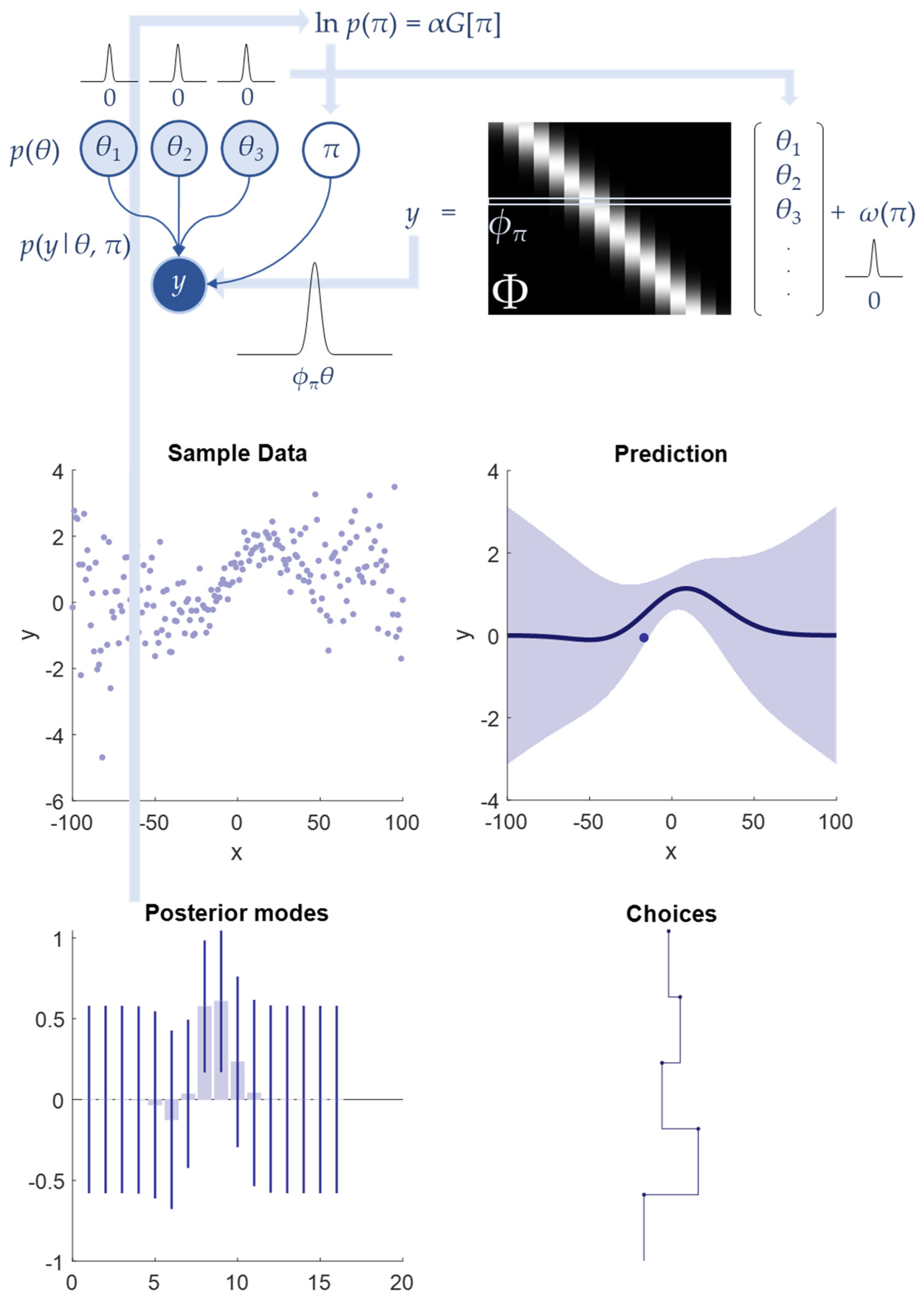
Figure 5 shows what happens when we select our data according to
G[π], where the preference for stopping sampling takes the value 1/4 (i.e.,
C = [0,…,0,1/4] includes zeros for all but the ‘stop sampling’ option, which is assigned a value of 1/4). This means that when the expected information gain is sufficiently low the chance of deciding to stop sampling increases.
In
Figure 5, we see that the same first 15 choices are made as in
Figure 4. However, at this point, a decision is made to stop sampling. This is because sufficient uncertainty has been resolved that the cost of sampling is greater than the potential information gain by sampling further. Depending upon how costly the sampling is assumed to be, this decision to stop will move earlier or later, and the quality of the function approximation will vary.
A reasonable question to ask at this stage is why bother with the full information-seeking objective? It is clear from
Figure 4 and
Figure 5 that all we need to do is choose to sample from the regions with greatest predicted variance, sequentially reducing that variance until it is minimal throughout the domain of the function being approximated [
32]. This suggests that the predictive entropy from Equation (2) is sufficient on its own (c.f., maximum entropy sampling [
33]). However,
Figure 6 offers a rebuttal to this with a process whose measurement noise increases in variance from the centre of the function domain. This means the amount of unresolvable uncertainty is heterogeneous throughout the domain of potential sampling. Were we to ignore this, the uncertainty left to resolve will always be greater than the cost of sampling. Using the full expected information gain tells us that, although there is uncertainty left, there is no information to gain, and allows for earlier termination of our sampling procedure. Furthermore, it leads to a methodical sampling strategy: sampling starts from the minimally ambiguous central location and fans out as local uncertainty is reduced until the capacity to resolve further uncertainty drops below the cost of acquiring further samples. This avoidance of sampling in ambiguous locations is sometimes referred to as a ‘streetlight effect’ [
34] (see [
35] for further discussion with models comprising categorical distributions), which occurs only in the presence of a full expected information gain objective. The streetlight effect is the tendency to search where data are generated in a minimally ambiguous way—i.e., under a streetlamp compared to searching elsewhere on a darkened street.
5. Dynamic Processes
In this section, we consider processes that evolve in time. For example, while the approach in
Section 3 might be appropriate for mapping out the heights of a mountain range, it would not be suitable for measuring (for example) weather conditions or tectonic activity in different locations across that terrain, as these will change with time (although see [
36,
37] for closely related approaches to placing static sensors for environmental monitoring). To move beyond a temporal snapshot, we must extend our models to include dynamics. There are many ways to do this. One could set up a hidden Markov model, whose states probabilistically evolve according to discrete transition probabilities [
38]. An alternative would be to formulate a model in terms of a differential equation that determines the time evolution of hidden states generating data [
39]. A final option is to extend the model we used in
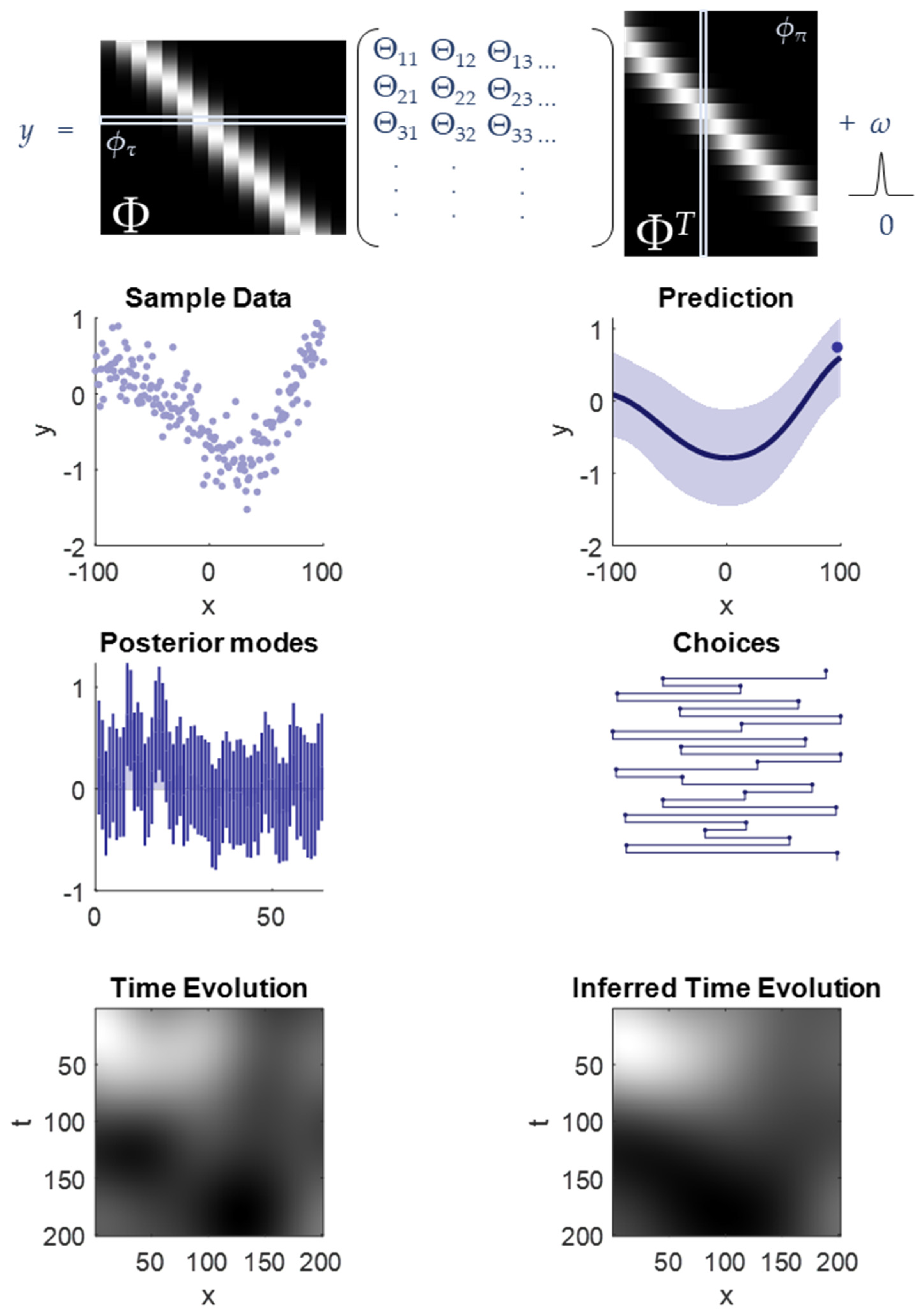
Section 4 to include a temporal dimension. Specifically, in place of our one-dimensional set of basis functions, we now use two-dimensional basis functions with both temporal and spatial components. While we employ the third of these methods in this paper, each of these three approaches is perfectly valid.
Equation (12) can be interpreted similarly to Equation (8), in which the expectation of the data is treated as a function approximation, which now includes a time argument.
However, the form of Equation (12) means we can use the same inferential machinery, and the same information gain calculations, as we did for the static inference examples.
Figure 7 shows a graphical representation of the matrices involved in generating our data and the inferences obtained after sampling. Every eight time steps, a sample is chosen to maximise the expected information gain, and this is used to update posterior beliefs exactly as previously. As can be seen from the lower-right panel in
Figure 7, an accurate inference has been obtained of the evolution of our function over time. The choices made when sampling provide a relatively even coverage of the spatial dimension. Note the implicit inhibition of return, which prevents resampling near recently sampled locations. However, once sufficient time has elapsed, it is worth returning to previously sampled locations as they may have changed since previously being sampled.
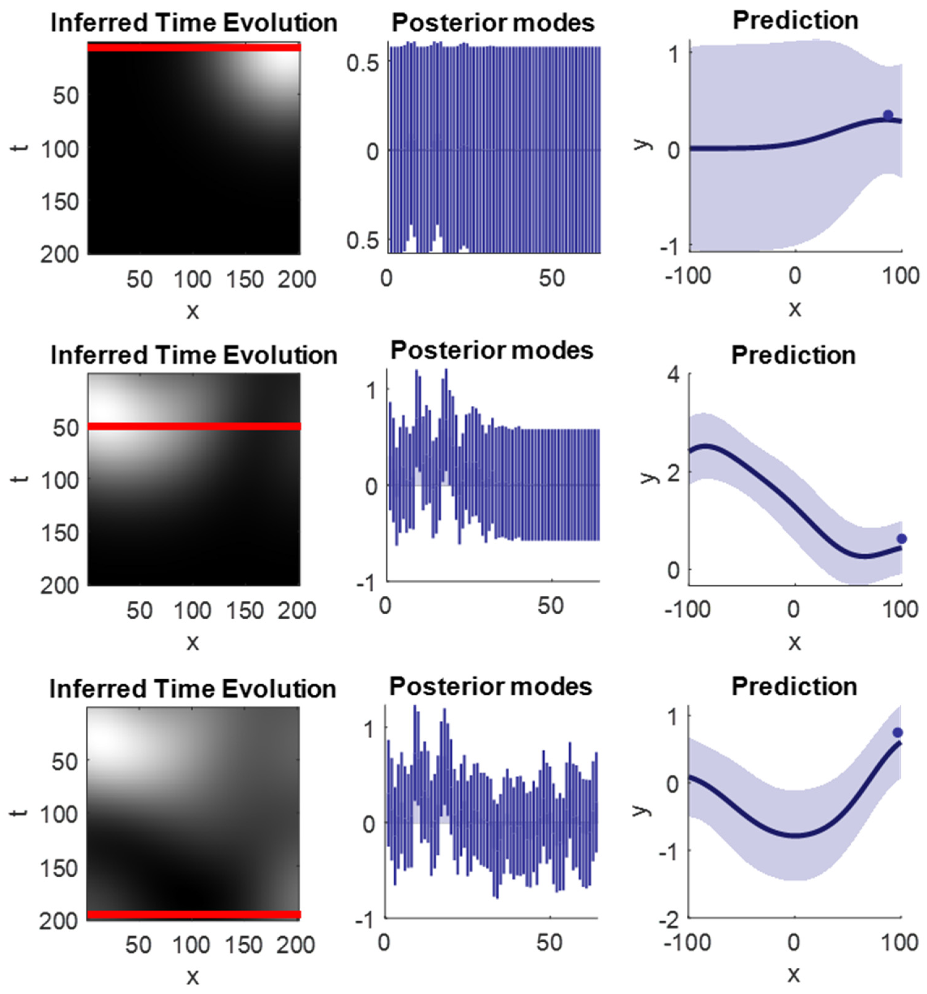
Figure 8 shows several snapshots of the inferences drawn at different time points during the simulation reported in
Figure 7. This is designed to provide some intuition as to the filling in of predictions as more observations are made. Note that because this is a dynamic process—with a degree of smoothness both in space and time—predictions based upon the current data can be used to inform predictions about nearby spatial locations and to both predict and postdict the values of the function at different points in time.
In this and the previous section, we have demonstrated the way in which smart or optimal sampling may be used to select data in a manner that balances the cost of sampling or of performing further experiments against the information gained from those samples or experiments. Each of these examples has relied upon relatively simple, and analytically comfortable, linear Gaussian systems. Next, we address active sampling in a situation where analytical solutions are no longer possible.
6. Clinical Trials
In our final example, we demonstrate the potential utility of the ideas outlined above in the context of a more concrete example. Adaptive Bayesian clinical trials [
40] have been increasingly popular in efficiently answering questions about medical interventions in rapidly evolving healthcare situations. A prominent example of this was the use of an adaptive Bayesian methodology to assess interventions during the 2014 West African Ebola outbreak [
41]. A key argument made in favour of this design was that in a rapidly developing epidemic it is necessary to be able to efficiently compare several possible treatments and to be able to adapt as new information emerges [
42]. For instance, we may wish to stop one treatment arm, or perhaps reallocate participants to another treatment arm, if there is early evidence of the inferiority or superiority of this treatment, respectively. These benefits are not restricted to the management of epidemics but may apply more broadly. See, for example [
43,
44,
45,
46,
47,
48,
49].
We have two reasons for choosing a clinical trial design as our final example. The first is that they are common hypothesis-driven experimental designs with resource limitations. The second is that they offer us an opportunity to go beyond the illustrative linear models used above and force us to deal with more expressive model structures that require pragmatic approximations to be able to apply the methods outlined above efficiently. Our hope is to demonstrate that use of expected information gain does not restrict us only to the simplest model classes but has broad applicability in real-world problems.
The active sampling approach advocated in this paper offers two main opportunities to augment adaptive trial designs. First, it allows us to adapt the design (e.g., inclusion criteria and assignment to a treatment arm) to maximise the information we obtain about treatment efficacy. Second, it allows us to balance this information gain against various costs, namely, stopping the trial when the potential information gain no longer exceeds the cost of acquiring further data. Alternatively, it might include a preference for good clinical outcomes and aversion for bad outcomes—prompting adjustments of the allocations between treatment arms to maximise benefit as we infer more about the effect of the intervention. This blurs the line between clinical trial and public health intervention and can be seen as analogous to animal behaviour that is never fully exploitative or explorative but is a balance between the two.
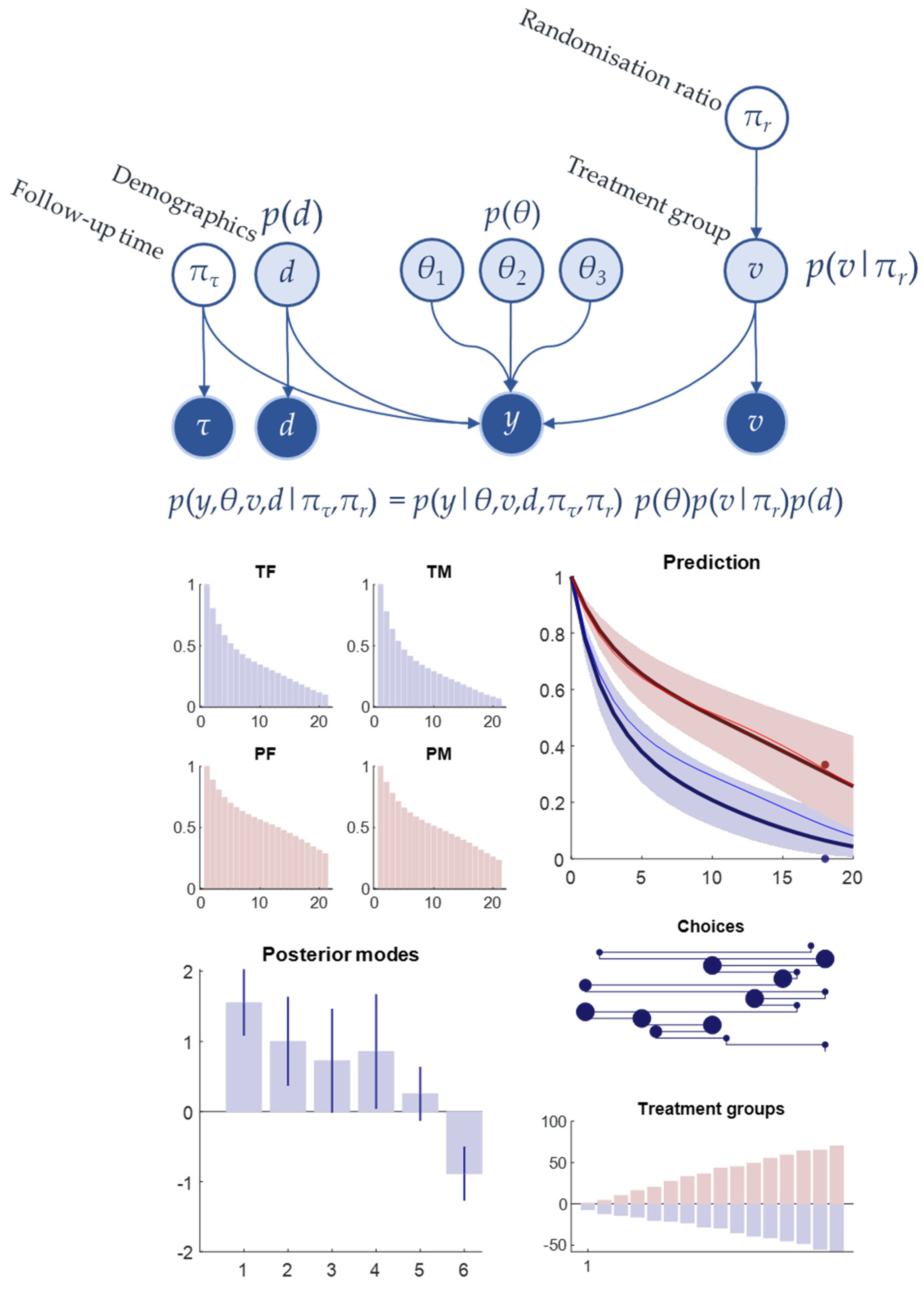
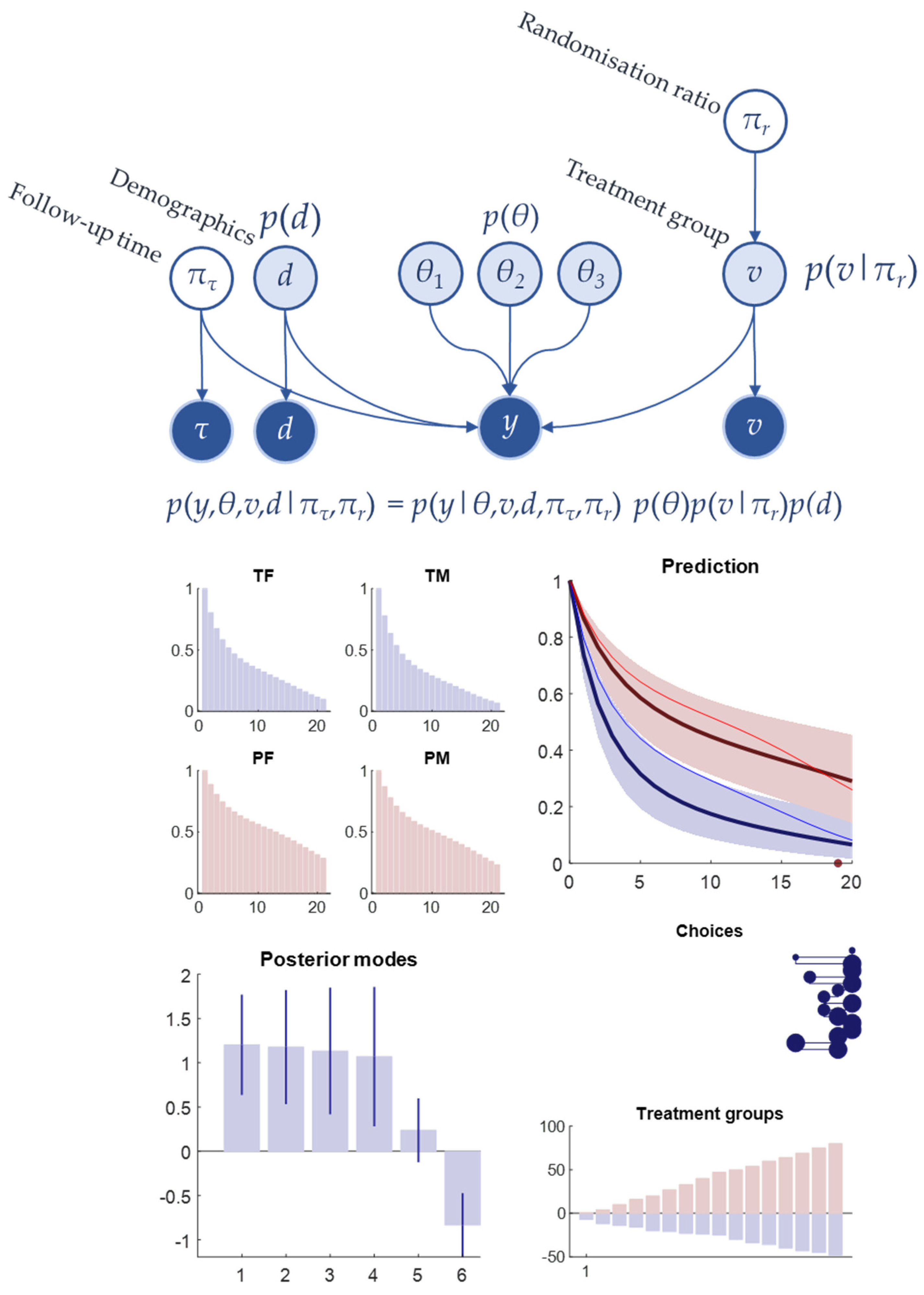
Our setup is as follows: for each new cohort of participants, we decide upon the randomisation ratio to adopt and the time(s) at which we follow them up. To simplify for illustration purposes, we assume each cohort is followed up only once, noting that the same principles can be applied to multiple follow-up points. Our generative model can be expressed as follows:
In this model, the data (
y) are binary values reflecting survival up to the measurement time or death before this point. The probability of survival to a given time is the product of the survival probabilities for all previous time steps. Our probability for survival for a given time step is a logistic function that determines the effect of time since enrolment in the trial, the effect of demographic (here, sex), and the treatment effect. As in our previous examples, the time evolution is modelled using a Gaussian basis set. Patient demographics (
d) are sampled from a categorical distribution. There are two choices that can be made. The first is the time at which follow up is performed (subscript
τ). The second is the randomization ratio (subscript
r). There are assumed to be three options for this ratio. These are 1/3, 1/2, or 2/3 allocated to the treatment group. The allocation is represented by the symbol
v. We assume these decisions are taken before each cohort, where each cohort consists of eight participants. The parameterisation of the treatment effect (i.e., the final element of
ϴ) can be interpreted as a hazard ratio, as might be estimated in a Kaplan–Meier [
50] analysis, and is consistent with Cox proportional hazards assumptions [
51].
This model differs from those in previous sections in that it includes highly nonlinear functions and is not based upon conjugate priors. This makes analytical solutions to the inference problem intractable. In place of this, we employ a variational approximation to arrive at posterior estimates. This involves a Newton optimization scheme (also known as Variational Laplace) applied to maximise a lower bound on the log marginal likelihood. The relevant gradient expression for this scheme is as follows:
The Hessian is as follows:
The variational optimization scheme then takes the form (where superscripts indicate iteration number)
Figure 9 shows a simulation of this design with random sampling of both follow-up time and randomization ratio. The variational inference scheme here terminates following 16 iterations. The upper part of the figure shows the form of the generative model as a Bayesian network. The process used to simulate data is summarised in the plots of survival against time for each of the combinations of treatment versus placebo and male versus female. In this example, the treatment is harmful, leading to a lower survival in the treatment compared to the placebo group. This pattern is captured by the inference scheme following 16 cohorts and a relatively even sampling throughout time and randomization patterns.
Next, we wish to employ the information gain prior, to deliberately choose follow-up times and randomization ratios to maximise our information about the trajectories of each patient group. As above, the first step in doing so is to identify the form of the messages required for Equation (3).
We can simplify the estimation of these messages using a local quadratic approximation for the continuous parameters. This technique is sometimes referred to as Variational Laplace and is implicit in Equation (17) [
52,
53].
For the messages in the first term of Equation (18), we employ a quadratic expansion of the entropy around the posterior mode of the parameters:
The second term of Equation (18) has the following form when the
ρ function has been expanded to the second order:
Please see Equations (15) and (16) for the forms of the relevant gradients and Hessians.
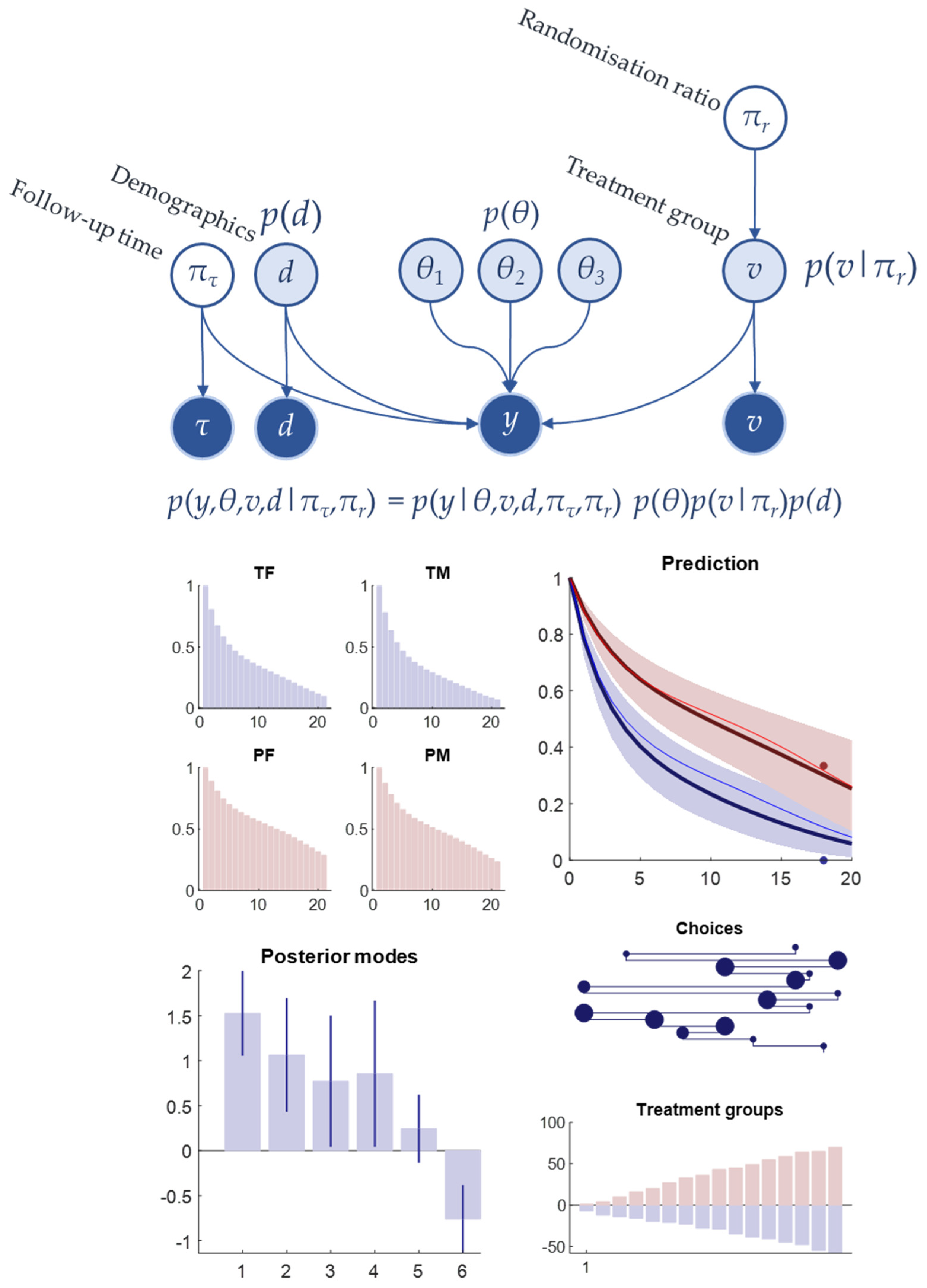
Figure 10 illustrates the same setup as in
Figure 9 but now using the expected information gain from Equation (18) to guide sampling of data. Due to the approximations made to ensure tractability, we reduce the temperature (i.e.,
α from
Figure 4) to four to acknowledge that there is some uncertainty as to whether the best choices are those consistent with the maximal value of Equation (18). There are some notable differences between the choices made in
Figure 10 compared to
Figure 9. The most obvious of these is that the follow-up times selected have been moved later once optimal sampling is employed. This makes intuitive sense as a later follow-up time is informative about the survival probabilities at all prior times, whereas an earlier follow-up time is not informative about survival probabilities at later times. This has led to a marginal improvement in estimation of the hazard functions. In both cases, the number of people assigned to each treatment group appears approximately equivalent, as would be expected under random sampling, with an expectation of 50% assignment to each group overall.
Our final simulation now incorporates the preferences discussed in previous sections. Here the preferences are expressed in terms of a prior probability that survival is more likely than death. This must be nuanced as a preference for observing survival alone would favour observations at the point of enrolment where the probability of survival is 100%. To finesse this problem, we specify a preference for survival that increases exponentially in time. In other words, it is preferable to observe somebody having survived until the end of the potential follow-up period compared to having observed their survival shortly after enrolment. As shown in
Figure 11, this preference for long-term survival results in longer follow-up times and, interestingly, once an inference that the treatment is potentially harmful has been made, there is a gradual shift towards randomising more people towards the placebo group. This implies a similar reasoning to when clinical trials are terminated early when a clear benefit of membership of one of the two treatment arms has been identified.
7. Discussion
This paper’s focus has been on illustrating how we might make use of information-seeking objectives—augmented with costs or preferences—to choose the best data to optimise our inferences. While we have highlighted specific examples of active sampling or optimal Bayesian design, we have not provided a systematic analysis of the benefits of this approach here—instead favouring demonstrations of application to different sorts of models and problems. We have considered the problem of function approximation when there is a cost to data acquisition, or to the computational demands when sampling data from large datasets. We extended this to consider dynamic inference when the data obtained from the same experiment, address, or abstract location may change as a function of the time at which they are acquired. Finally, we illustrated the use of these methods even when the problem is not reducible to a general linear model.
It is worth noting that several of our examples would yield identical results had we adopted a data-sampling approach based upon maximum entropy sampling [
54,
55]. However, the key differences emerge when the variance around predicted outcomes is inhomogeneous. We illustrated this both in the static inference example in
Figure 6 and also in our clinical trial example. Note that the covariance associated with the likelihood distribution is a function of the Hessian of the log likelihood. Equation (15) shows that this is not constant in the nonlinear setting considered in our final example.
There are several technical points worth considering for how we might advance the concepts reviewed in this paper. These are broadly: (1) refinement of the active selection process, (2) empirical evaluation of active versus alternative sampling methods, and (3) identifying the appropriate cost functions. Sophisticated inference is a method that might address the first of these [
56]. This deals with the situation in which there is a dependence between the information gained from one choice and the potential information that can be gained following future decisions. In addition to this, it can help prioritise those sources of information that minimise cost in the future. Essentially this involves solving a recursive planning problem, like the approach used to solve Bellman optimality problems. The utility of sophisticated recursions is obvious when we consider how we would approach a clinical trial with multiple follow-up points, as the timing of the second follow-up will depend upon the information gain we anticipate from the first.
The issue of empirical validation is one that can be addressed through two routes. The first is in selecting a limited number of samples from a large dataset through either an active sampling approach or through some alternative data selection strategy. By using the posterior probability distributions under each sampling strategy as priors and comparing the marginal likelihood for the two sets of priors—assessed against the remainder of the dataset—we could evaluate the sampling strategy that leads to the best model. The second route to assessing the utility of active sampling is through comparing the energy costs and computing time required to achieve a reasonable approximation of a function using a limited dataset compared to that required to take account of a larger and more comprehensive dataset.
The identification of appropriate cost functions may be a trickier problem as these will vary from application to application and with the resources available. This has particular significance for clinical trial design, where the relative preference for different outcomes clearly has important ethical connotations. One approach would be to reverse-engineer the implicit cost functions employed in previous experimental designs (for example, the cost functions that would lead to a given early stopping criteria). An alternative is to find a way to synthesise and formalise views from the relevant stakeholders. For an interesting example of this in the context of determining outcomes for cystic fibrosis trials, see [
57,
58].


