Field Programmable Gate Array-Based Acceleration Algorithm Design for Dynamic Star Map Parallel Computing

Abstract

The dynamic star simulator is a commonly used ground-test calibration device for star sensors. For the problems of slow calculation speed, low integration, and high power consumption in the traditional star chart simulation method, this paper designs a FPGA-based star chart display algorithm for a dynamic star simulator. The design adopts the USB 2.0 protocol to obtain the attitude data, uses the SDRAM to cache the attitude data and video stream, extracts the effective navigation star points by searching the starry sky equidistant right ascension and declination partitions, and realizes the pipelined displaying of the star map by using the parallel computing capability of the FPGA. Test results show that under the conditions of chart field of view of $\mathrm{\Phi }20°$ and simulated magnitude of $2.0\sim 6.0 \mathrm{Mv}$, the longest time for calculating a chart is 72 μs under the clock of 148.5 MHz, which effectively improves the chart display speed of the dynamic star simulator. The FPGA-based star map display algorithm gets rid of the dependence of the existing algorithm on the computer, reduces the volume and power consumption of the dynamic star simulator, and realizes the miniaturization and portable demand of the dynamic star simulator.

1. Introduction

A star sensor is an instrument that determines the attitude of a vehicle in real time by means of an optical system, star point extraction, and star map recognition. It is one of the attitude sensors with the highest measurement accuracy [1]. Compared with solar and earth sensors, star sensors have a wider range of applications in the fields of navigation, aerospace, and aviation [2]. Therefore, star sensor technology has been at the forefront of international attention [3].

With the development of the aerospace industry, the demand for high-precision and real-time star sensors is increasing day by day [4]. As the dynamic star simulator is the ground-test calibration equipment for star-sensitive instruments, the improvement of its star map display speed can improve the efficiency of star map identification by star sensors. In 2013, Wu, X.M. et al. [5] designed an electronic star simulator based on DSP (Digital Signal Processing) and FPGA (Field Programmable Gate Array) by utilizing a two-stage chain-list indexing approach to search for 9006 stars in the range of 0 Mv~6.5 Mv, and the average speed of a star map display was about 56 ms. In 2022, Hao, G.N. et al. [6] searched for 15,914 stars from −2.0 Mv to 7.0 Mv in a star map field of view of $20°\times 20°$ using an externally tangent circular partition search algorithm, and a single star map showed an average velocity of about 9.43 ms. In 2021, Li, G.X. et al. [7] used the navigational star leveling method to search for 5103 stars from 2.0 Mv to 6.0 Mv under a star chart field of view of $10°\times 10°$. A star chart showed an average velocity of about 7.98 ms.

Based on the current development of dynamic star simulators, it can be concluded that most of the dynamic star simulators are computers that transmit data directly to the star chart display module after performing three parts, namely, solving attitude data, searching for navigational stars, and coordinate transformation. On the one hand, the computer is large in size and high in power consumption, which is not convenient to test the star sensor at any time; on the other hand, if the computer adopts serial computing, then the instructions of the processor can only be executed sequentially, and only one instruction can be executed at most at a single moment. The DSP has the ability to perform high-speed computing [8], but it is not suitable for complex logic operations [9], and the code is cumbersome. The FPGA can be customized to meet the user’s needs with the required modules [10] to reduce the cost and development difficulties [11].

In recent years, in the context of the continuous development of dynamic star simulation technology, the refresh rate of the star chart has been a key indicator of the dynamic characteristics of dynamic star simulators. The higher the refresh rate of a star map, the less time it takes for the required star map to be calculated. As the ground calibration equipment of the star sensitizer, in the practical application of the star simulator, some experiments will need to be simulated outdoors. In outdoor environments, portability, miniaturization, and low-power systems are also among the current research trends. Aiming at the above problems of low real-time and slow calculation speed based on the serial structure of the dynamic star simulator chart display algorithm, this paper designs a dynamic star simulator star map display algorithm based on FPGA, which determines the position of the optical axis in the whole sky area by calculation on the FPGA platform and then displays the navigational stars within the field of view through coordinate transformation. The design of this paper improves the speed of the dynamic star chart display. It is significant for the development of miniaturization and the high real-time performance of dynamic star simulators.

2. System Components

The overall block diagram of the FPGA-based dynamic star simulator star map display algorithm is shown in Figure 1. It is mainly composed of the following four parts: optical axis calculation, navigation star search, coordinate transformation, and star map display. LCOS (Liquid Crystal on Silicon) in Figure 1 is a commonly used display device for dynamic star simulators.

3. Digital Star Chart Generation

3.1. Starlist Pre-Processing

The star catalogues are the catalogues that record the parameters of celestial bodies and contain the most basic data for generating star charts, including information about the celestial bodies in the celestial coordinate system such as right ascension, declination, and star. In order to reduce the number of subsequent calculations, the star catalogs are preprocessed into two parts: grayscale transformation and star partitioning.

3.1.1. Grayscale Transformation

In this paper, the information about right ascension, declination, and magnitude are adopted to draw the star map, and the simulated magnitude range is from 2.0 Mv to 6.0 Mv, so the other information in the catalog and the star points outside the simulated magnitude range are excluded. The British astronomer Pogson stipulated that the difference between the magnitudes of neighboring stars is 2.512 times [12], assuming that there are two stars with magnitudes $m_0$ and $m_i$ and brightnesses $E_0$ and $E_i$, and their correlation is as follows:

$$\frac{E_{\mathrm{i}}}{E_0}={2.512}^{m_0-m_i}$$

(1)

The relative relationship between the brightness of the two stars is shown in Equation (1), and the brightness of the star points is displayed by controlling the gray value of the pixels of the LCOS [13]. The computer grayscale is represented by 8-bit data, with each pixel point gray value being in the range of 0~255. It is specified that the 2 Mv star point grayscale is 255, and the relationship between the grayscale $g_i$ of the rest of the stars and other $m_i$ is shown in Equation (2) as follows:

$$g_i=\frac{255}{{2.512}^{m_i-2}}$$

(2)

3.1.2. Star Partitioning

Star partitioning is a method of further subdividing all the stars in the SAO (Smithsonian Astrophysical Observatory) catalogues into a smaller range of sky zones according to the right ascension and declination, which reduces the search range of the star chart and avoids searching for all the star point information in the chart in order to subsequently speed up the search for navigational stars. In this paper, the dynamic star simulator star map display algorithm is designed with a field of view angle of $\mathrm{\Phi }20°$, which is divided according to the partition interval B = 12°, taking into account the effect of attitude offset and the factor of reducing the number of target star subzones [14]. The right ascension varies from 0° to 360° and is divided into 30 zones; the declination varies from −90° to 90° and is divided into 15 zones, totaling 450 target subzones. The 450 target subzones are numbered according to the order of high to low declination and small to large declination, and the star zoning map is shown in Figure 2.

3.2. GNSS Search and Coordinate Transformation

The attitude of the vehicle can be represented by quaternions [15] and Euler angles. Due to the high complexity of the FPGA’s computing trigonometric functions, this paper uses quaternions to represent the attitude of the vehicle. The algebraic form of quaternion $q$ is shown in Equation (3) as follows:

$$q_0=q_1\overrightarrow{i}+q_2\overrightarrow{j}+q_3\overrightarrow{k}+q_4$$

(3)

where $q_1$, $q_2$, and $q_3$ are vector values of $q$, and $q_4$ is a scalar value of $q$.

The canonical quaternion has a constraint relationship, as shown in the following Equation (4):

$${q_1}^2+{q_2}^2+{q_3}^2+{q_4}^2=1$$

(4)

The attitude transformation matrix $C$ expressed in quaternions is shown in Equation (5) as follows:

$$C=\left[\begin{array}{ccc}1-2{q_2}^2-2{q_3}^2& 2\left(q_1{q}_2+q_3{q}_4\right)& 2\left(q_1{q}_3-q_2{q}_4\right)\\ 2\left(q_1{q}_2-q_3{q}_4\right)& 1-2{q_1}^2-2{q_3}^2& 2\left(q_2{q}_3+q_1{q}_4\right)\\ 2\left(q_1{q}_3+q_2{q}_4\right)& 2\left(q_2{q}_3-q_1{q}_4\right)& 1-2{q_1}^2-2{q_2}^2\end{array}\right]$$

(5)

The z-axis pointing of the attitude transformation matrix is the direction of the optical axis of the star sensor, so the direction vector of the optical axis pointing is obtained in the matrix ${\left[\begin{array}{ccc}{x}_0& y_0& z_0\end{array}\right]}^T$ as shown in the following Equation (6):

$${\left[\begin{array}{ccc}{x}_0& y_0& z_0\end{array}\right]}^T={\left[\begin{array}{ccc}2\left(q_1{q}_3+q_2{q}_4\right)& 2\left(q_2{q}_3-q_1{q}_4\right)& -{q_1}^2-{q_2}^2+{q_3}^2+{q_4}^2\end{array}\right]}^T$$

(6)

The expression of the right ascension and declination vector in spatial Cartesian coordinates in the celestial coordinate system is shown in the form of Equation (7) as follows:

$${\left[\begin{array}{ccc}X& Y& Z\end{array}\right]}^T={\left[\begin{array}{ccc}\cos \delta \cos \alpha & \cos \delta \sin \alpha & \sin \delta \end{array}\right]}^T$$

(7)

where $\alpha$ and $\delta$ are the values of the right ascension and declination of the star point.

Let ${\left[\begin{array}{ccc}{X}_s& Y_s& Z_s\end{array}\right]}^T$ be the spatial Cartesian coordinate direction vector of the star sensor, and the conversion relationship with the direction vector of the star point in the celestial sphere coordinate system is shown in Equation (8) as follows:

$$\left[\begin{array}{ccc}{X}_s& Y_s& Z_s\end{array}\right]=C{\left[\begin{array}{ccc}X& Y& Z\end{array}\right]}^T$$

(8)

Let the star sensor optical axis pointing be the right ascension and declination $\left({\alpha }_0,{\delta }_0\right)$, and the expression can be obtained from Equation (9) as follows:

$$\left\{\begin{array}{l}{\alpha }_0=\left\{\begin{array}{l}\arctan \frac{y_0}{x_0}+2\pi ,\left(x_0>0,y_0<0\right)\hfill \\ \arctan \frac{y_0}{x_0},\left(x_0>0,y_0\ge 0\right)\hfill \\ \frac{\pi }{2},\left(x_0=0,y_0>0\right)\hfill \\ \frac{3\pi }{2},\left(x_0=0,y_0<0\right)\hfill \\ \arctan \frac{y_0}{x_0}+\pi ,\left(x_0<0\right)\hfill \end{array}\right.\hfill \\ {\delta }_0=\arcsin z_0\hfill \end{array}\right.$$

(9)

The star area zone filtering can improve the speed of the navigation star search according to the optical axis of the star sensor to point to the target subzone range within the search range, which is sufficient.

The left ($J_l$) and right ($J_r$) boundaries of the star area subarea numbers are calculated as shown in the following Equation (10):

$$\left\{\begin{array}{c}{J}_l=\mathrm{int}\left(\frac{\alpha -\left(\frac{R}{2}\right)/cos\delta -180°}{B}+\frac{M}{2}\right)\\ J_r=\mathrm{int}\left(\frac{\alpha +\left(\frac{R}{2}\right)/cos\delta -180°}{B}+\frac{M}{2}\right)\end{array}\right.$$

(10)

If $J$ is not in the interval 0 to 29, it is added or subtracted by continuously adding or subtracting 30 until $J$ falls within the interval 0 to 29. The upper ($D_u$) and lower ($D_d$) bounds of the star area sub-area numbering are calculated [16] as shown in the following Equation (11):

$$\left\{\begin{array}{c}{D}_u=\mathrm{int}\left(\frac{\delta +\frac{R}{2}}{B}+\frac{N}{2}\right)\\ D_d=\mathrm{int}\left(\frac{\delta -\frac{R}{2}}{B}+\frac{N}{2}\right)\end{array}\right.$$

(11)

If $D$ < 0, then $D$ is taken as 0; if $D$ > 14, then $D$ is taken as 14. $M$ and $N$ are the maximum values of the numbering of the star zones according to the right ascension and declination, respectively, and $B$ is the interval of the star zones.

Let $\theta$ be the angle between the direction of the star point and the direction of the optical axis, and FOV be the field-of-view angle of the star sensor, and the formula for its angle is shown in the following Equation (12):

$$\arccos \theta =\frac{x_1{x}_2+y_1{y}_2+z_1{z}_2}{\sqrt{{x_1}^2+{y_1}^2+{z_1}^2}\cdot \sqrt{{x_2}^2+{y_2}^2+{z_2}^2}}$$

(12)

If $\theta \le FOV/2$, the point is within the star sensor’s field of view and is a valid point. If $\theta >FOV/2$, the point is invalid. After screening the valid star points, the coordinates in the celestial coordinate system need to be converted to the coordinates of the pixel points on the LCOS plane, which can be obtained according to the resolution of the LCOS and the field of view of the star sensor as follows:

$$\left\{\begin{array}{l}x=f\cdot \frac{X_1}{Y_1}\hfill \\ y=f\cdot \frac{Z_1}{Y_1}\hfill \end{array}\right.$$

(13)

$$f=\frac{n}{2}\cdot \frac{1}{\tan \left(\frac{R}{2}\right)}$$

(14)

In Equations (13) and (14), $X_1$, $Y_1$, and $Z_1$ are the coordinates of the star point in the star sensor coordinate system; f is the focal length; R is the field of view angle; and n is the number of pixel points in the row or column of the LCOS.

3.3. Star-Point Diffuse Spot Generation

The star point in a star chart is not a uniformly distributed bright spot; it is a bright spot that approximates a diffuse spot. The energy of the bright spot becomes a two-dimensional Gaussian distribution, which is expressed as follows in Equation (15).

$$g\left(x,y\right)=\frac{A}{2\pi {\sigma }^2}\exp \left(-\frac{{\left(x-X\right)}^2+{\left(y-Y\right)}^2}{2{\sigma }^2}\right)$$

(15)

where $g\left(x,y\right)$ is the gray value of the pixel point at pixel coordinates $\left(x,y\right)$;$\left(X,Y\right)$ is the coordinates of the center position of the star point; A is the total gray value of the star point; and $\sigma$ is the size of the diffuse spot radius of the image point, usually $\sigma$ taken as 0.45 [5], in which case about 90% of the energy can be distributed in the $3\times 3$ pixel matrix.

4. FPGA-Based Hardware and Software Architecture Design

This paper is based on the Vivado 2018.3 development environment on the ACX720 development board using Xilinx’s XC7a35tfgg484-2 as the FPGA master chip. The quaternion attitude data are outputs from the star sensor, which is simulated to produce a dynamic star map in the field of view of the star sensor after the attitude data are solved by the dynamic star simulator.

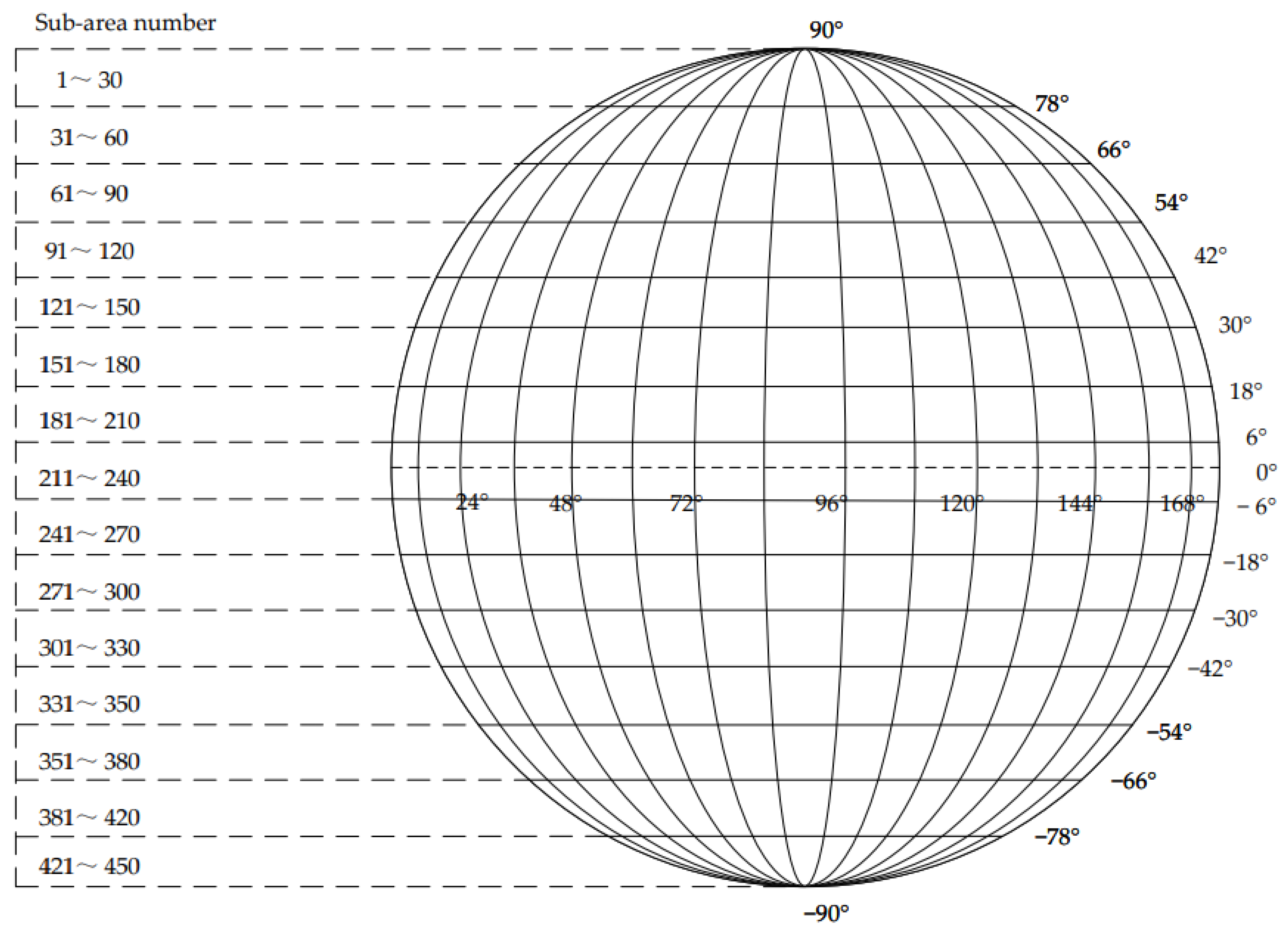
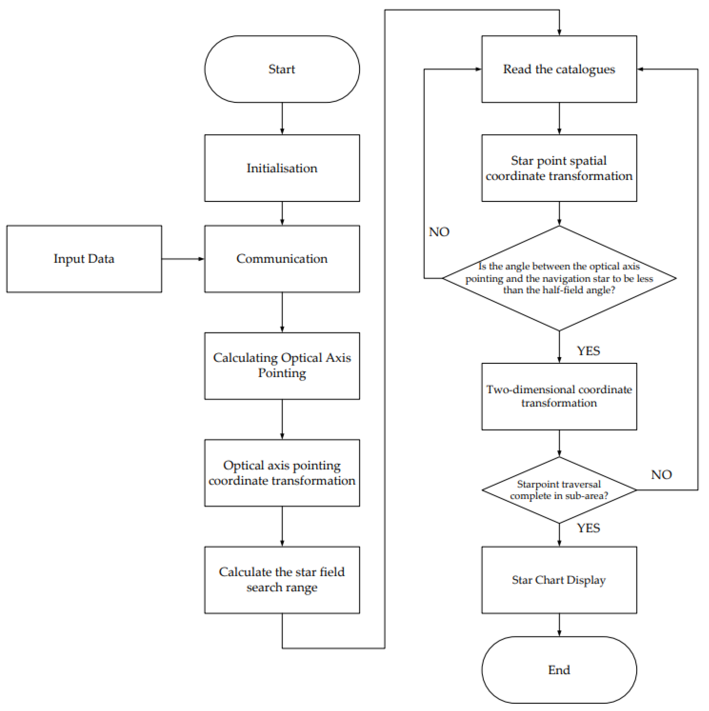
The Dynamic Star Simulator chart display algorithm initializes each module, waits for the attitude quaternion data to be sent by the star sensor, and calculates the spatial right-angled coordinate direction vector of the optical axis pointing expressed as a quaternion through the attitude transformation. The optical axis pointing is converted from a spatial right-angle coordinate direction vector to a celestial sphere coordinate direction vector to confirm the target subarea within the field of view.

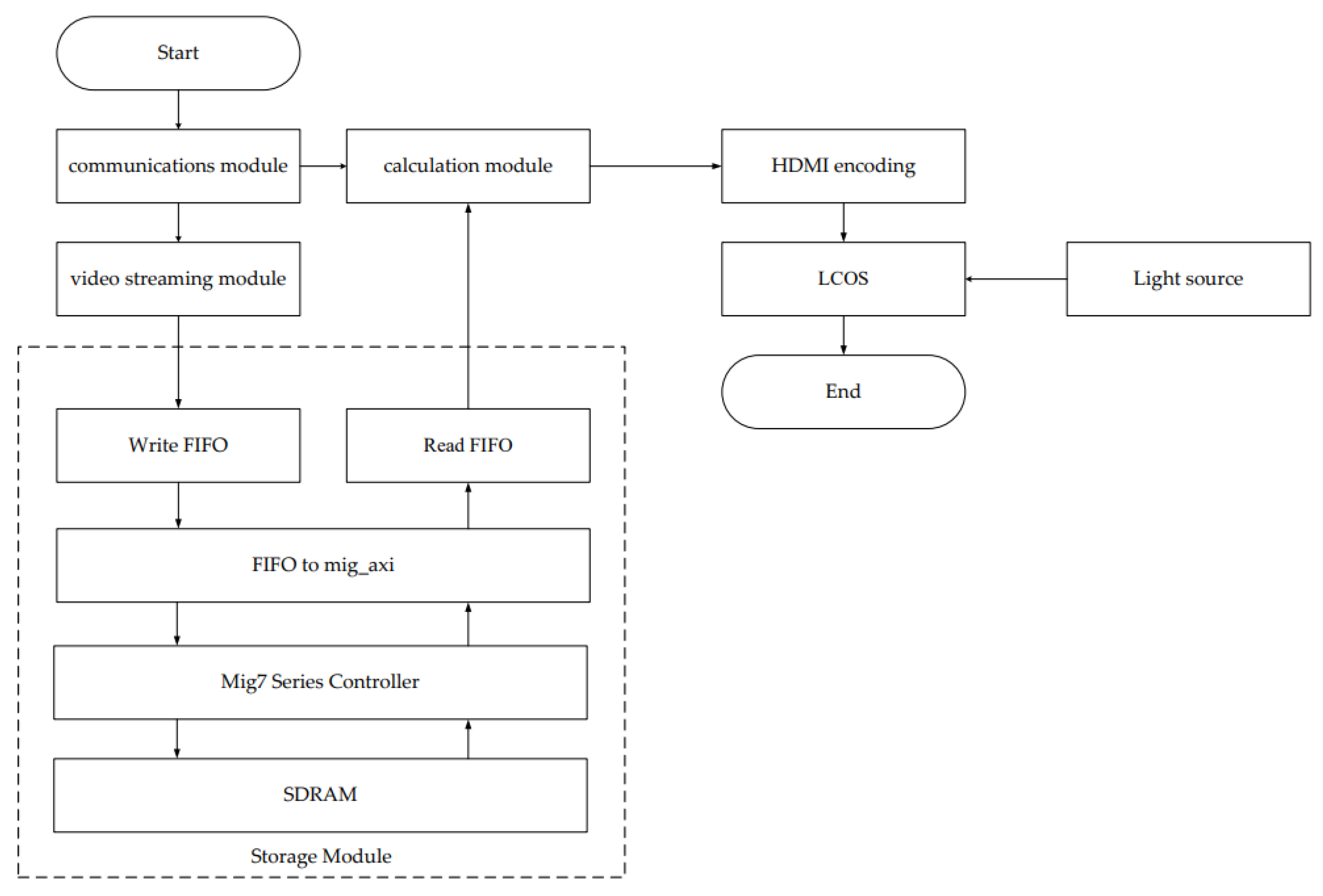
After that, the FPGA reads the preprocessed star catalog data, converts the celestial coordinates of the star point into spatial Cartesian coordinates, and calculates the coordinate angle between the vector direction of the optical axis and the vector direction of the star point. If this star point is judged to be a valid star point, then the star point’s star sensor coordinates to the two-dimensional plane rectangular coordinates of the transformation; otherwise, it is judged to be an invalid star point; continue to read the next star point; and finally, all the valid star points together to form a star map. The flow chart of the dynamic star chart display algorithm is shown in Figure 3.

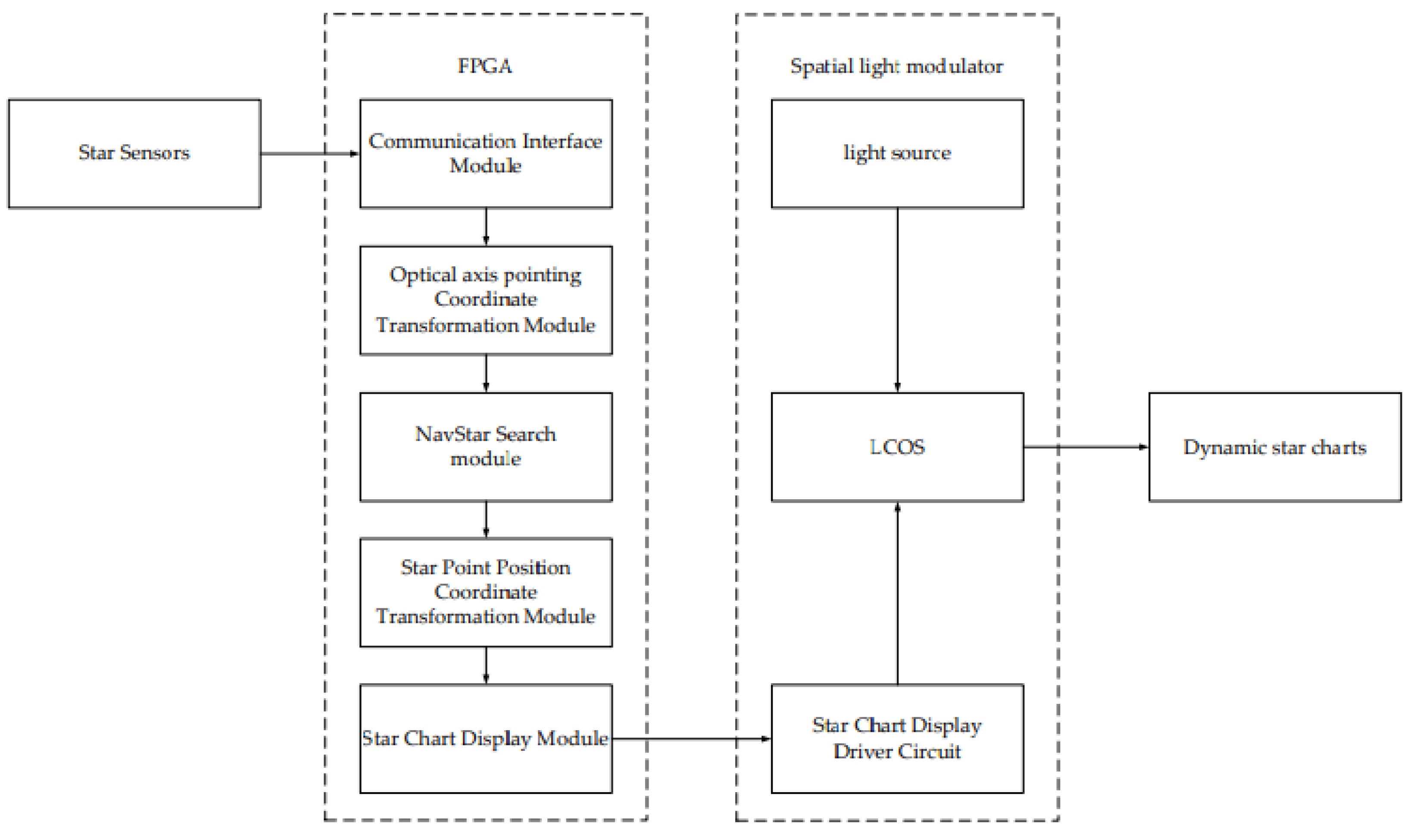
The hardware architecture of the dynamic star simulator is mainly composed of a communication module, a computation module, and a storage module [17]. The modular design can process the computed star map in a flow, as shown in Figure 4, which shows the FPGA data flow structure.

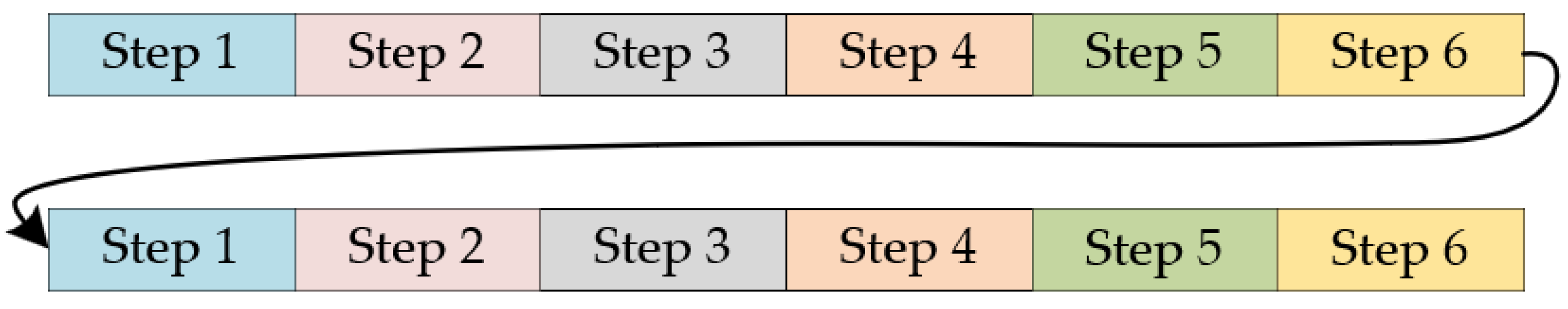
The schematic diagram of using the serial computation method on a conventional computer platform is shown in Figure 5. It is necessary to carry out all the steps in the calculation to complete it, and then rerun the next calculation. The advantage of the serial calculation method is that the structure is relatively simple compared to the parallel calculation method, and it is the main calculation method used in the current star chart display method.

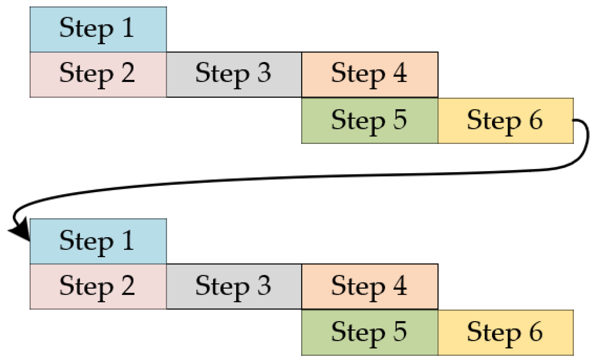
Figure 6 is a schematic diagram of FPGA parallel computation [18], where the steps can be adder, subtractor, multiplier, and other steps. In the calculation process, as in the relationship between step 4 and step 5 in Figure 5, if step 5 does not need the calculation result of step 4, then steps 4 and 5 can be calculated in parallel.

In executing the computational star map algorithm, four computational modules are available in parallel on the FPGA platform. The optimized results obtained are shown in

Table 1. Parallel analysis of computational modules.

Computational Module	Parallel Part	Time Saved in Parallel Part
5.1	Adder/Subtractor and Multiplier	290 ns
5.3	Adder/Subtractor	60 ns
5.5	Adder/Subtractor and Square Calculator	60 ns
5.6	Adder/Subtractor, Multiplier, and Square Calculator	40 ns

. No. 5.1 is a simulation of waveforms for optical axis pointing calculations. No. 5.3 is a simulation of waveforms for star field search range calculation. No. 5.5 is a simulation of waveforms for star point coordinate transformation calculation. No. 5.6 simulation waveform of star point coordinate transformation.

4.1. Calculation Module

The input and output signals of the calculation module include the enable signal of the video stream, the line synchronization signal, the field synchronization signal, and the grayscale signal. The function of this module is to use the quaternion signal inputted from the serial port to calculate and obtain the star catalog data within the target sub-area; calculate the right ascension, declination, and star magnitude in the star catalog data to obtain the x-direction coordinate, y-direction coordinate, and the grayscale value of the pixel point; and finally, replace the pixel by pixel one by one according to the coordinates [19].

The main clock of the FPGA chip is 50 MHz, and the 148.5 MHz pixel clock is used in the calculation module [20]. There is a process of transmitting data across the clock domain in the communication, and it is necessary to add two levels of triggers to synchronize the signals for transmitting the data to prevent the phenomenon of race and hazard from occurring.

The attitude data is calculated to determine the target subarea boundaries and the attitude transformation matrix, with the target subarea numbering increased from $30D_i+J_l$ to $30D_i+J_r$ where $D_i$ is increased from $D_u-1$ to $D_d-1$. If the optical axis is pointing at an angle of $\theta \le FOV/2$ to the star point, the star point active enable signal oi_en is raised, and the coordinates of the star point are read when the target subarea where the star point data is located is within the boundary and the star point active enable signal is high and reads the star point coordinates pix_x and pix_y.

In the effective star point judgment, the judgment condition is replaced by the equivalent of the formula, which is more suitable for FPGA processing. From Equation (12), the valid star point judgment condition can be obtained as follows from Equation (16):

$$\arccos \theta =\frac{x_0{x}_1+y_0{y}_1+z_0{z}_1}{\sqrt{{x_0}^2+{y_0}^2+{z_0}^2}\cdot \sqrt{{x_1}^2+{y_1}^2+{z_1}^2}}\le \frac{FOV}{2}$$

(16)

Since the approximate orientation of the star point has been determined in the previous steps by means of star partitioning, $\arccos \theta$ should lie within $0°\sim 90°$, which falls within the monotonically decreasing interval of the cos function, so it can be obtained by Equation (17) as follows:

$${\left[\cos \left(\frac{FOV}{2}\right)\right]}^2\cdot \left({x_0}^2+{y_0}^2+{z_0}^2\right)\cdot \left({x_1}^2+{y_1}^2+{z_1}^2\right)\le {\left(x_0{x}_1+y_0{y}_1+z_0{z}_1\right)}^2$$

(17)

Calculations are performed using fixed-point decimal calculations, which saves the use of IP cores and reduces computation time compared to floating-point decimal operations. In conventional gesture data calculations, quaternion data in decimal generally retains four significant digits, i.e., thirteen significant digits in binary. Quaternion data values, right ascension and declination values, and trigonometric functions are calculated with values less than 10, and fixed-point arithmetic with 1 integer and 13 decimal places is used in the data calculation, where the bit width of the resultant data from the quadratic operation needs to be twice the width of the previous base data. Thus, a 26-bit reg variable is required in the quadratic operation. The divisor is implemented using IP cores, and the bit-widths of the divisor and divisor need to be greater than or equal to the bit-width of the result of the quadratic operation. The divisor is therefore implemented using IP cores, with both the divisor and dividend set to 32 bits wide and the quotient set to 64 bits wide. The trigonometric function calculation uses the LUT lookup table method to reduce the complexity of the algorithm, where angle-related data use 2 bits wide and 12 bits wide.

4.2. Storage Module

The memory module consists of three IP cores, wr_fifo, rd_fifo, and u_mig_7series_0, and the FIFO-to-mig_axi module. The FIFO is in between the computation module and the FIFO to mig_axi because the clock and transfer rate are different between the modules, so the data is cached in the FIFO, and the data is read and written in the DDR through the FIFO interface to the AXI interface. It can realize the function of reading and writing data in DDR through the FIFO interface to the AXI interface.

The wr_fifo and rd_fifo write and read data are input video streams. wr_fifo uses the development board operating clock of 50 MHz, with the write width set to 16 bits and the write depth set to 512 bits. rd_fifo uses the ui_clk clock of 200 MHz output from the MIG IP, with the read width set to 128 bits and the read depth set to 64 bits.

The memory controller is based on Xilinx’s MIG IP cores to meet the high-capacity, high-speed DDR3 SDRAM memory, where the AXI bus under the Xilinx platform is suitable for the development of various IP cores.

The AXI interface bus has a total of five channels, namely, read address channel (RD_ADDR), read data channel (RD_DATA), write address channel (WR_ADDR), write data channel (WR_DATA), and write response channel (WR_RESP), and each AXI transmission channel is a unidirectional channel.

AXI lite is more suitable for communication between the FPGA main chip and peripherals than AXI full. In this paper, the arbitration module of the FIFO interface to the AXI interface is designed based on mig’s AXI interface. The initial state after power-on is IDLE, and after waiting for init_calib_complete to go high after DDR initialization is completed, it enters the read/write arbitration state ARB, after which the conversion between the FIFO interface and the AXI interface is carried out in accordance with the operating state transition diagram of the read/write transaction, as seen in Figure 7. The state transfer conditions are shown in

Table 2. State transfer condition table.

State Transfer Number	State Transition Condition
1	init_calib_complete = 1
2	rd_ddr3_req == 1’b1
3	m_axi_arready && m_axi_arvalid = 1
4	m_axi_rready && m_axi_rvalid && m_axi_rlast && (m_axi_rresp == 2′b00) && (m_axi_rid == AXI_ID)
5	wr_ddr3_req == 1’b1
6	m_axi_awready && m_axi_awvalid = 1
7	m_axi_wready && m_axi_wvalid && m_axi_wlast = 1
8	m_axi_rready && m_axi_rvalid && (m_axi_bresp == 2′b00) && (m_axi_bid == AXI_ID)

.

4.3. Pixel Point Display Module

The calculated star point coordinates pix_x, pix_y, and pix_gray are cached through registers to obtain mem_x, mem_y, and mem_gray. The number of registers can be configured according to the number of star points to be displayed in the predicted star map. Eighty registers are used for caching in this project. In the display module, the pixels are scanned one by one in a display plane with a resolution of $1920\times 1080$ by control of line synchronization signals and field synchronization signals. The disp_x and disp_y signals are compared with mem_x and mem_y, respectively, and an enable signal is output when the signal levels are the same. When the enable signal is valid, pre_red, pre_green, and pre_blue are replaced with mem_gray, which in turn completes the replacement of the gray value of the pixel point. A complete star map can be obtained through the above process. During the display of the dynamic star map, the line synchronization signal and field synchronization signal will continuously scan the pixel points one by one to achieve the effect of the dynamic star map.

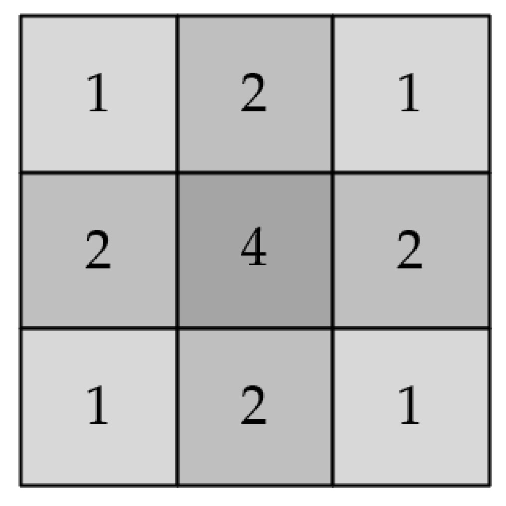
The grayscale distribution of the star-point diffuse spots conforms to a two-dimensional Gaussian distribution. In a Gaussian distribution, about 90% of the energy is distributed in the interval $\left(\mu -2\sigma ,\mu +2\sigma \right)$. At the same time, considering the way binary data is processed, a $3\times 3$ Gaussian filter template with weight assignment, as shown in Figure 8, is used in the project.

The module caches $3\times 3$ templates by calling two RAM-base Shift Registers to cache pixel rows in series. The cached data is calculated by the Gaussian filtering formula, as shown in Equation (18). The data flow diagram for Gaussian filtering is shown in Figure 9.

$$g\left(x_0,y_0\right)={\displaystyle \sum _{j=y_0-1}^{j=y_0+1}{\displaystyle \sum _{i=x_0-1}^{i=x_0+1}\frac{f\left(x_i,y_j\right)\cdot a_{ij}}{16}}}$$

(18)

where $g\left(x_0,y_0\right)$ is the gray value of the pixel point after filtering, and $a_{ij}$ is the weight assigned by the template.

5. Simulation Debugging

5.1. Algorithm Accuracy Analysis

In order to verify the effectiveness of the above algorithm, the algorithm is used to simulate the dynamic star map under the MATLAB R2022a software environment, and the simulation is carried out with resolutions of $q_1=0.109382,$ $q_2=0.234570,$ $q_3=0.875246,$ and $q_4=0.408218$. The coordinates and grayscale of the pixels of the star points in the star map are obtained. The star catalog global traversal algorithm and the algorithm in the literature [16] are simulated in MATLAB, and the results of the computation of the pixel coordinates are retained to four digits after the decimal point. The calculations show that all 45 star points are present, so there are no missing star points. Some of the star points are calculated as shown in

Table 3. Calculation of star points.

Star Point Number	Algorithms of the Article	Global Traversal Algorithm	Algorithms in Literature [16]
1	(1344, 52)	(1343.6290, 52.3454)	(1343.1869, 52.4629)
2	(1061, 140)	(1060.8745, 140.0319)	(1060.5171, 140.6719)
3	(916, 118)	(916.4424, 118.2077)	(916.2079, 118.7047)
4	(856, 59)	(856.3491, 58.9552)	(856.1927, 59.4249)
5	(1831, 458)	(1830.8544, 457.6822)	(1830.6509, 457.8170)
6	(1788, 571)	(1788.0021, 570.7881)	(1787.8998, 571.2094)
7	(1760, 525)	(1760.3848, 524.7738)	(1760.0700, 524.7066)
8	(1620, 470)	(1619.9463, 469.7154)	(1619.8961, 470.1568)
9	(1507, 301)	(1506.5255, 301.4758)	(1506.4625, 301.9288)
10	(1441, 319)	(1440.7954, 318.6252)	(1440.2570, 319.1484)
11	(1426, 428)	(1426.2083, 427.5948)	(1426.0594, 428.0663)
12	(1372, 273)	(1371.7320, 273.2372)	(1371.4097, 273.7248)
13	(1335, 261)	(1335.0012, 261.1535)	(1334.6780, 261.6318)
14	(1341, 289)	(1340.8006, 288.8830)	(1340.2432, 289.0485)
15	(1738, 597)	(1737.6861, 597.0918)	(1737.6717, 597.5124)
16	(1613, 768)	(1613.1615, 768.0119)	(1613.1064, 767.9271)

.

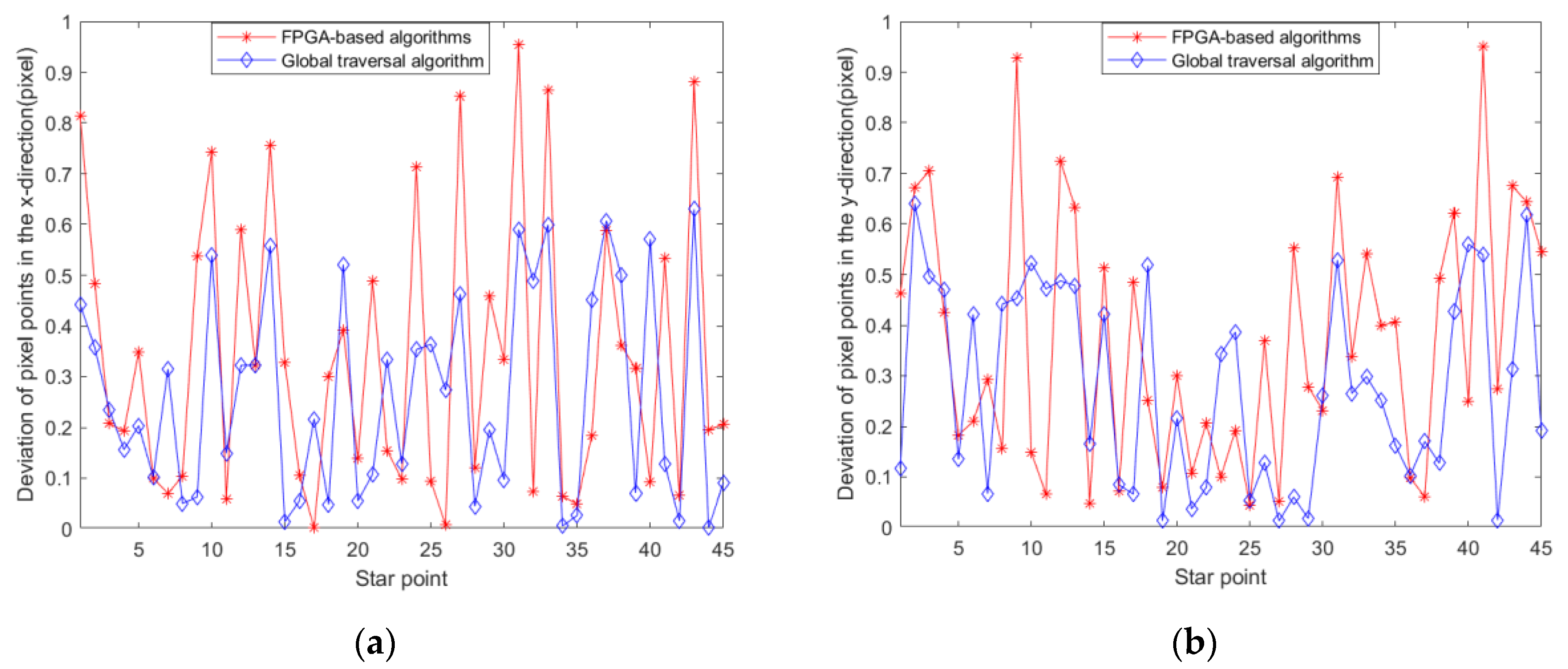
The computational results of the algorithms in the article and the global traversal algorithm are subtracted from the results of the algorithm in the literature [16] to obtain the deviation values, respectively. Figure 10a,b represent the deviation of the computational results of the algorithm in this article and the global traversal algorithm in the x-axis and y-axis directions, respectively.

By analyzing the digital star map generation method, the positional deviation of the star point pixels is generated by the following three main factors:

• Deviations arising from insufficient precision of the right ascension and declination.
• Deviations arising from insufficient precision of the quaternion.
• Deviations during lookup tables and divider computation on FPGA-based platforms.

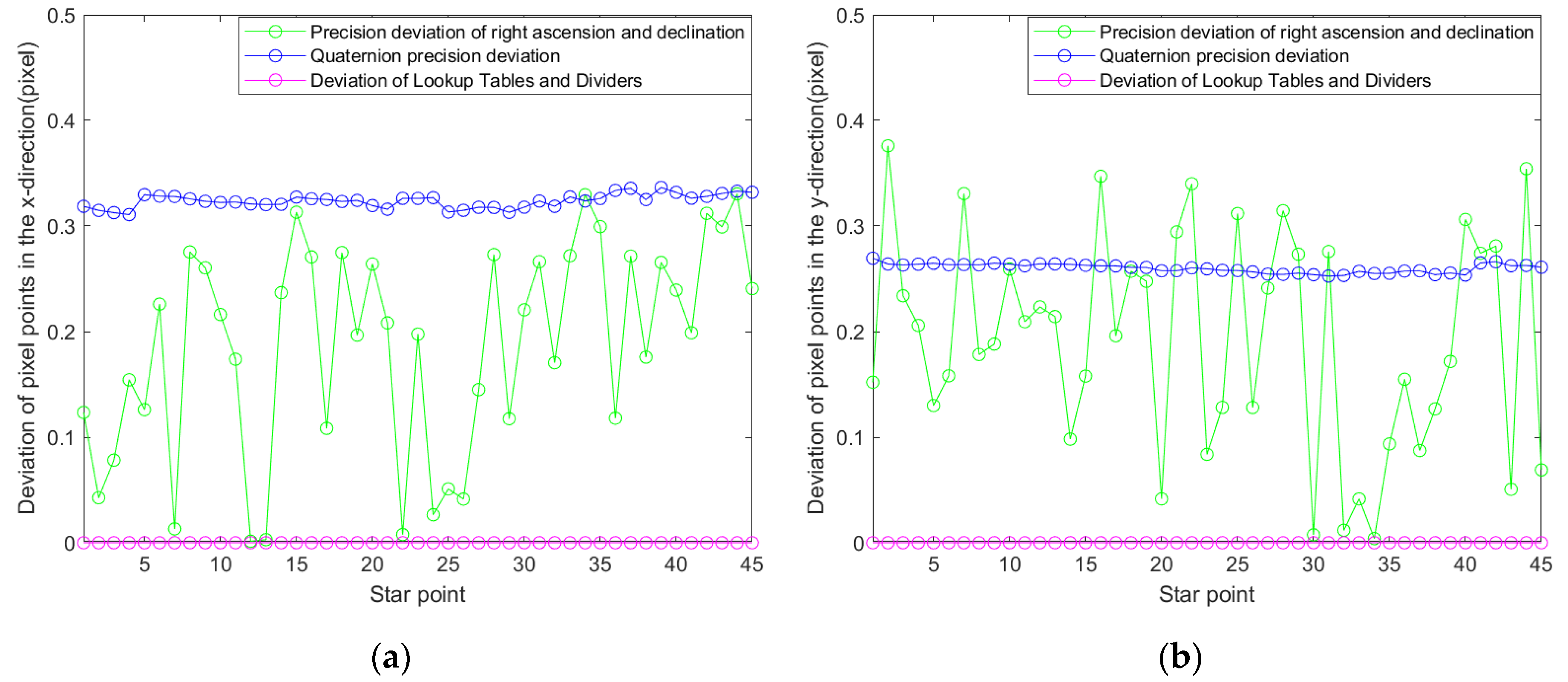
In MATLAB, Figure 11a,b are obtained by adding each of the three deviations separately to the algorithm of the literature [16]. The precision of the right ascension and declination produces a high deviation between the different star points. The mean values of deviation in the x-axis direction and the y-axis direction are 0.1874 and 0.1917, respectively. The deviation of the quaternion causes a deviation in the calculation of the optical axis pointing; therefore, its error produces a small overall shift in all the star points in the chart. The precision of quaternions produces a higher average deviation. The mean values of deviation in the x-axis direction and the y-axis direction are 0.3236 and 0.26, respectively. The lookup tables and the dividers have little effect on the final result during the calculation.

In summary, the algorithm in this paper deviates no more than one pixel point from the computed results of other algorithms. The deviation mainly comes from the error generated by the precision of right ascension and declination and the precision of quaternion. The deviation of the algorithm is less, which verifies the accuracy of the algorithm in this paper.

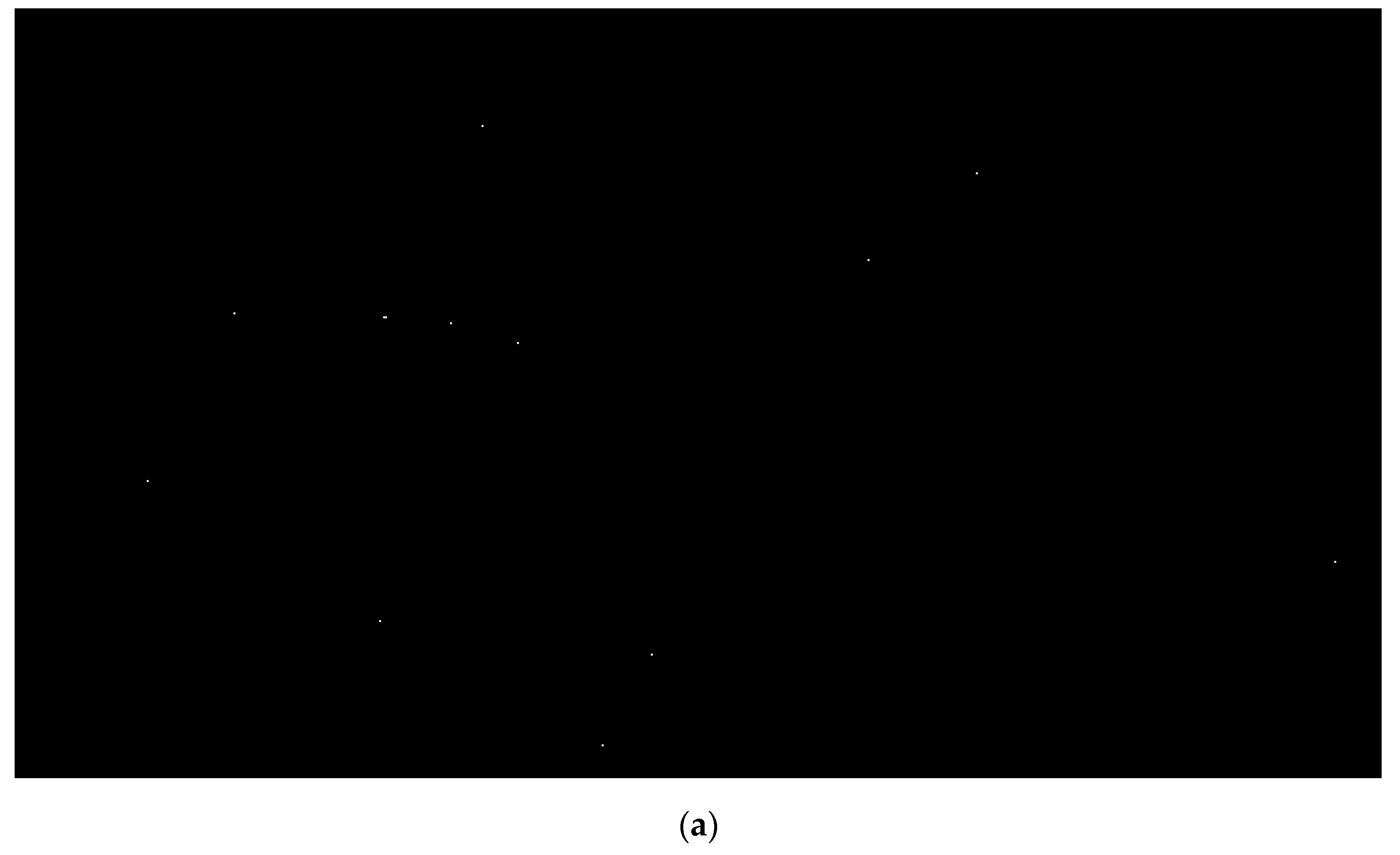
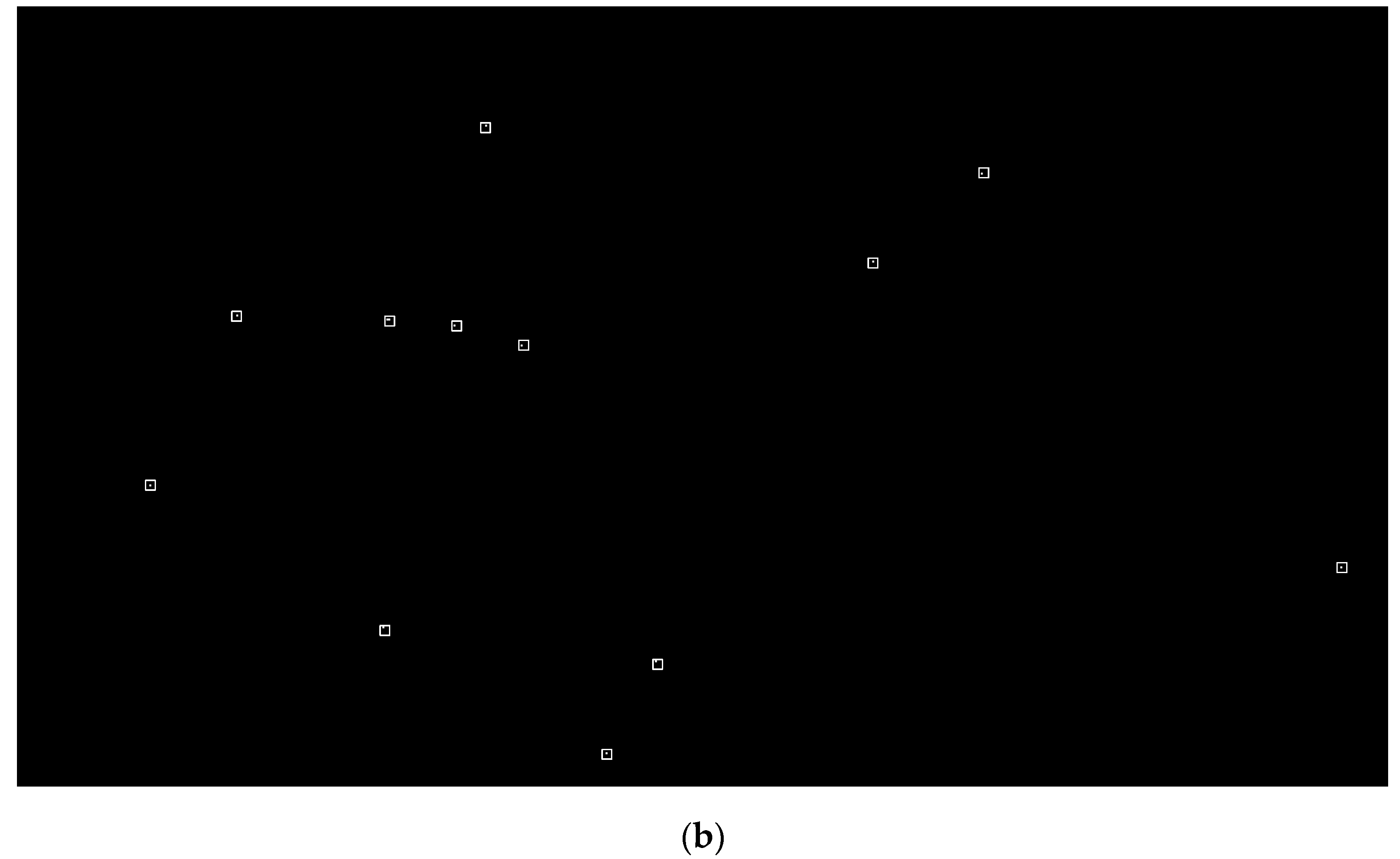
In MATLAB, the pixel matrix grayscale of the star map background is set to 0, and then by replacing the grayscale values of the pixels corresponding to the coordinates of the star points, a star map with a resolution of $1920\times 1080$ is generated. The simulation results are shown in Figure 12a,b, which highlights the star points in Figure 12a with boxes.

5.2. Simulated Waveforms for Optical Axis Pointing Calculation

The algorithm is used for waveform simulation on the FPGA platform. According to the VESA standard, the pixel clock of $1920\times 1080@60Hz$ is 148.5 MHz. Testbench uses a 100 MHz simulation clock in the waveform simulation in order to facilitate the simulation calculations.

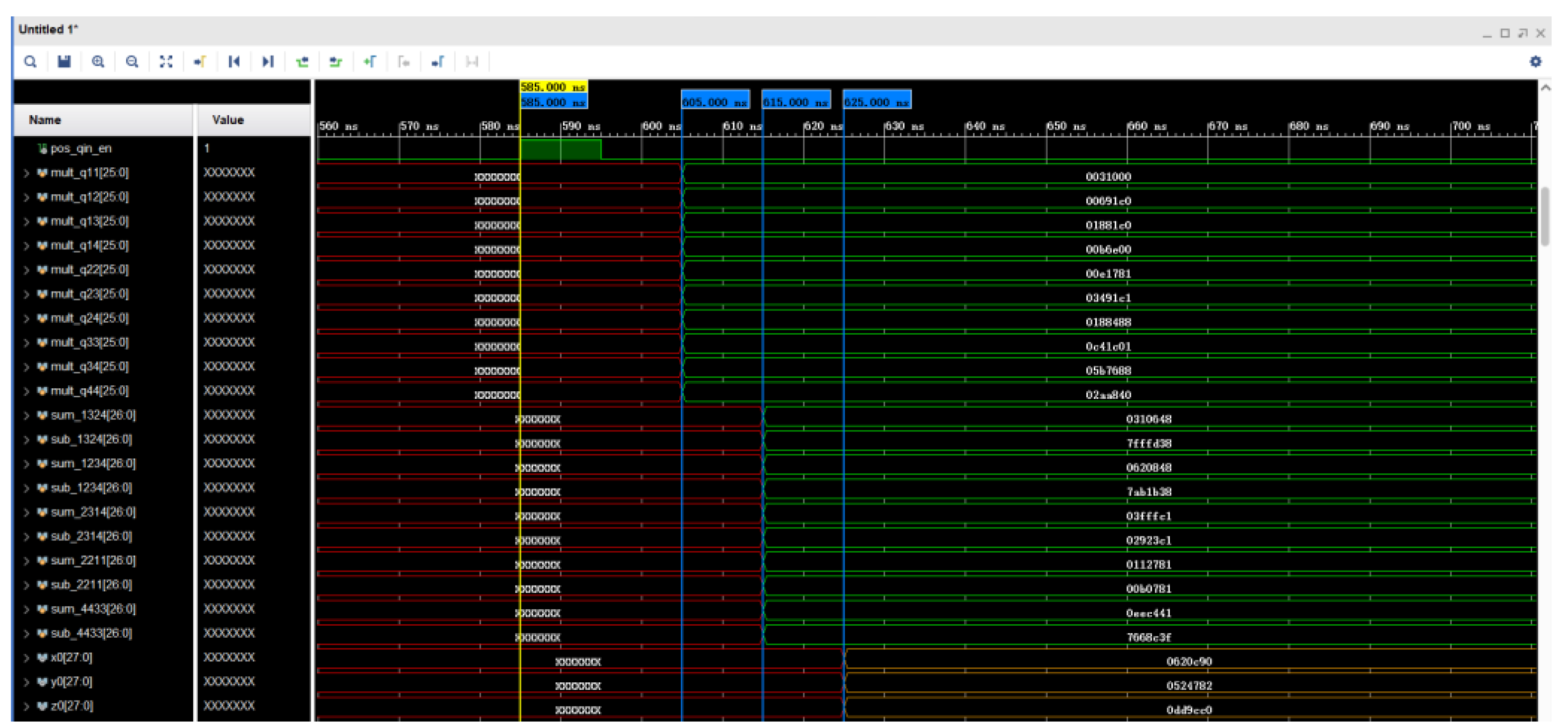
The simulation of the optical axis pointing calculation waveform is shown in Figure 13. Pos_qin_en is the enable signal for the input quaternions $q_1$, $q_2$, $q_3$, and $q_4$ from the upper computer. The signals named in the figure beginning with mult are multiplication operations of quaternions; the signals named beginning with sub and sum are addition and subtraction operations; and register x₀, register y₀, and register z₀ are the three elements of the optical axis pointing to the space vector. Waveform simulation results show that 10 multipliers complete the computation at 605 ns, 10 adders or subtractors complete the operation at 615 ns, and three elements of the optical axis pointing to the space vector are obtained at 625 ns, which is in accordance with the computation of Equation (6). The parallel computation of the FPGA here consumes 40 ns, which would consume 330 ns if a fully serial computation method were used.

5.3. Simulated Waveforms for Optical Axis Pointing Coordinate Transformation Calculation

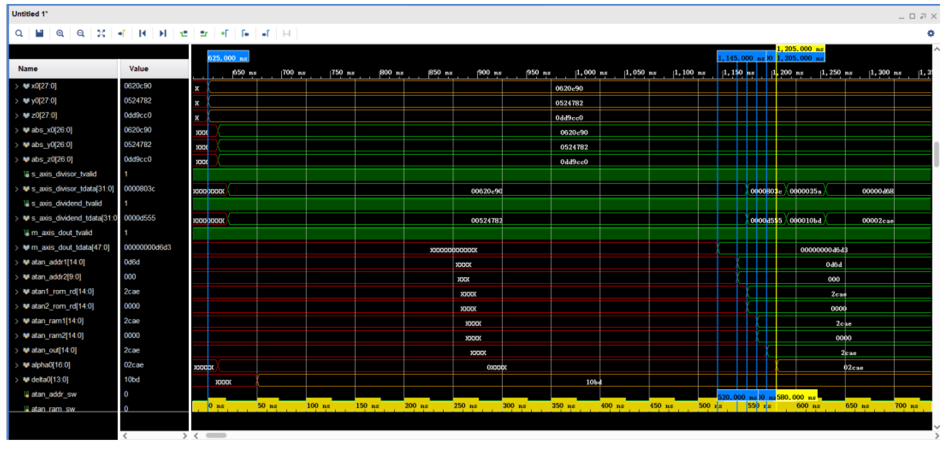
The simulation of the optical axis pointing coordinate transformation waveform is shown in Figure 14. The optical axis pointing ${\left[\begin{array}{ccc}{x}_0& y_0& z_0\end{array}\right]}^T$ completes the calculation process at 625 ns. The divider IP core uses about 500 ns, and then the table lookup method is used to calculate the value of atan to obtain the values of ${\alpha }_0$ and ${\delta }_0$ at 1205 ns in accordance with the calculation of Equation (9). The FPGA consumes 580 ns for the calculation here.

5.4. Simulated Waveforms for Star Field Search Range Calculation

The simulation of the star-area search range calculation waveform is shown in Figure 15. The ${\alpha }_0$ and ${\delta }_0$ trigonometric values are obtained by the look-up table method. At 1785 ns and 1795 ns, four adders or subtracters complete the calculation, which is in accordance with the calculation of Equations (10) and (11). In the simulation waveforms, the values of the four registers Jl, Jr, Du, and Dd are shown in decimals for ease of understanding. The parallel computation by the FPGA here consumes 590 ns, compared to 650 ns if the full serial computation method is used.

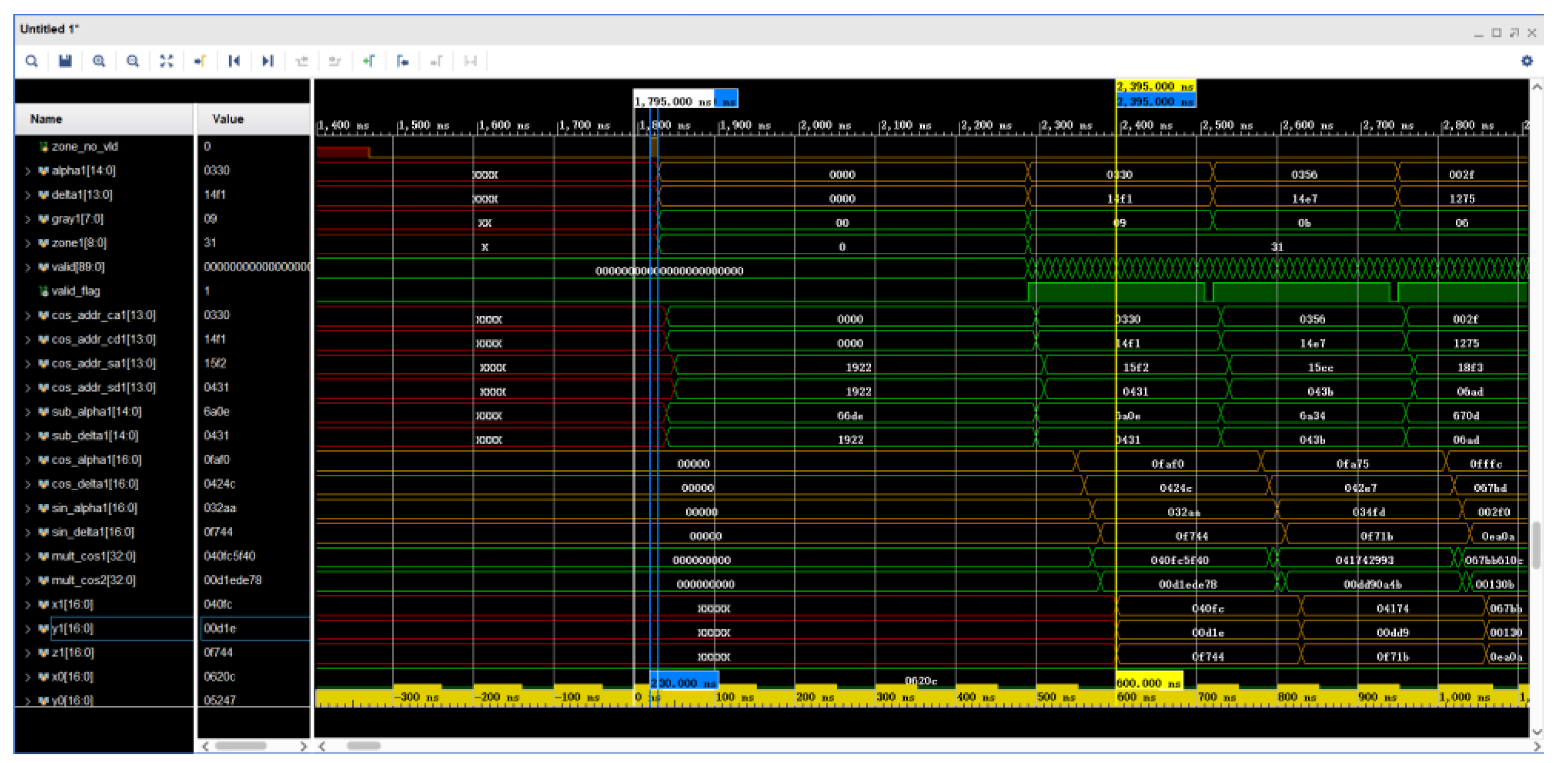
5.5. Simulated Waveforms for Star Point Coordinate Transformation Calculation

The simulation of the star point coordinate transformation calculation waveform is shown in Figure 16. The calculation is completed at 2395 ns by converting the star point coordinates represented by ${\alpha }_1$ and ${\delta }_1$ in the sub-area range to ${\left[\begin{array}{ccc}{x}_1& y_1& z_1\end{array}\right]}^T$ by means of a look-up table, indicating that the calculation conforms to Equation (7). Moreover, 600 ns are consumed by the FPGA for the calculation.

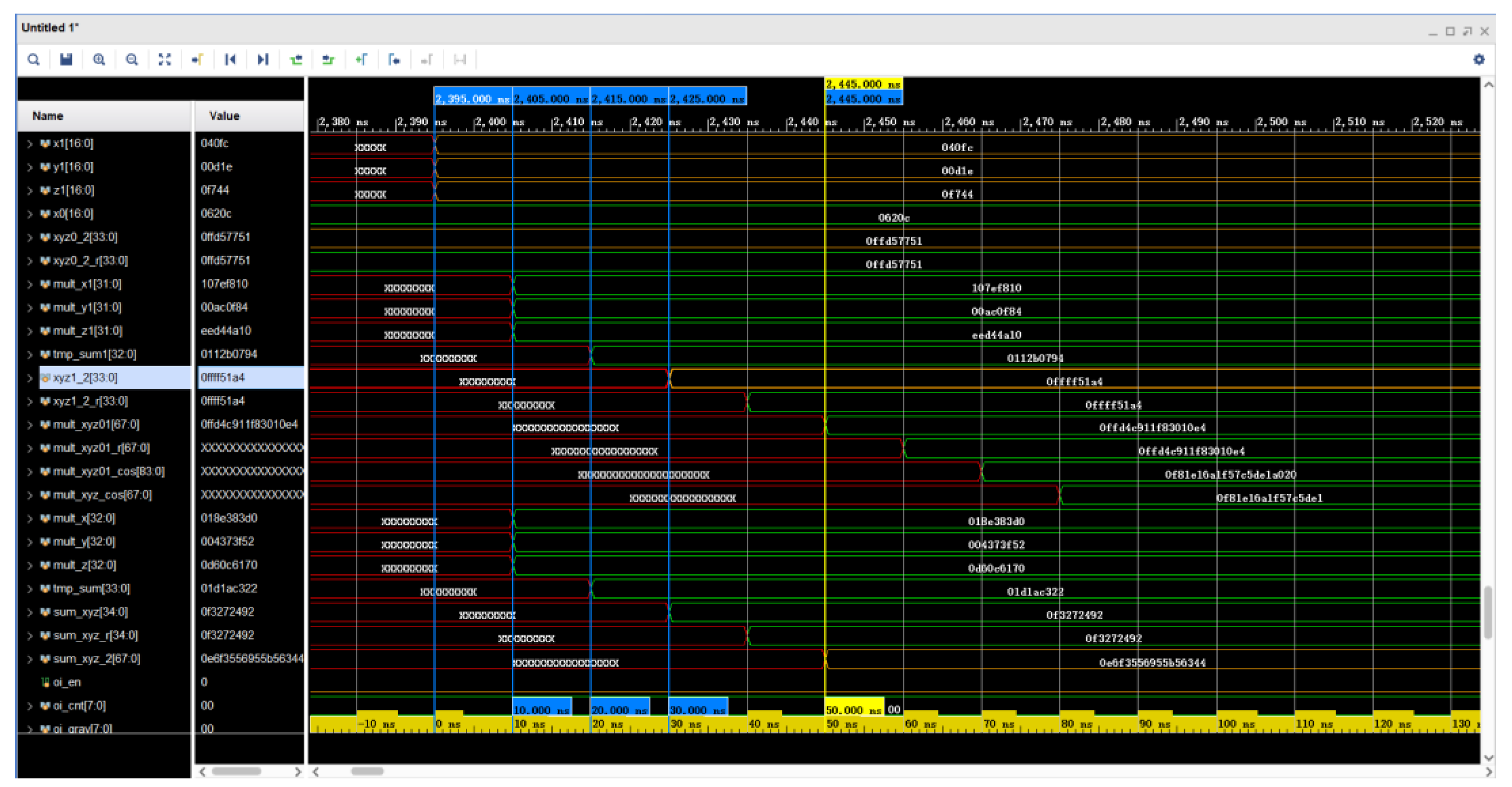
5.6. Simulated Waveforms for Star Point Coordinate Transformation Calculation

The simulation diagram of the effective judgment waveform of the star point is shown in Figure 17. On the basis of Equation (16), Equation (17) can be introduced. The values of register xyz0_2 and register xyz1_2 in the figure are the results of the calculation of ${x_0}^2+{y_0}^2+{z_0}^2$ and ${x_1}^2+{y_1}^2+{z_1}^2$, respectively. The value of register sum_xyz_2 is the result of the calculation of $x_1{x}_2+y_1{y}_2+z_1{z}_2$. At 2405 ns, six multipliers complete the operation. At 2415 ns, two adders completed their operations. At 2425 ns, two adders have completed their operations in parallel. All the calculations required for the star point judgment were completed at 2445 ns. The FPGA consumed 50 ns for the parallel calculations here, as opposed to 110 ns if a fully serial calculation method was used.

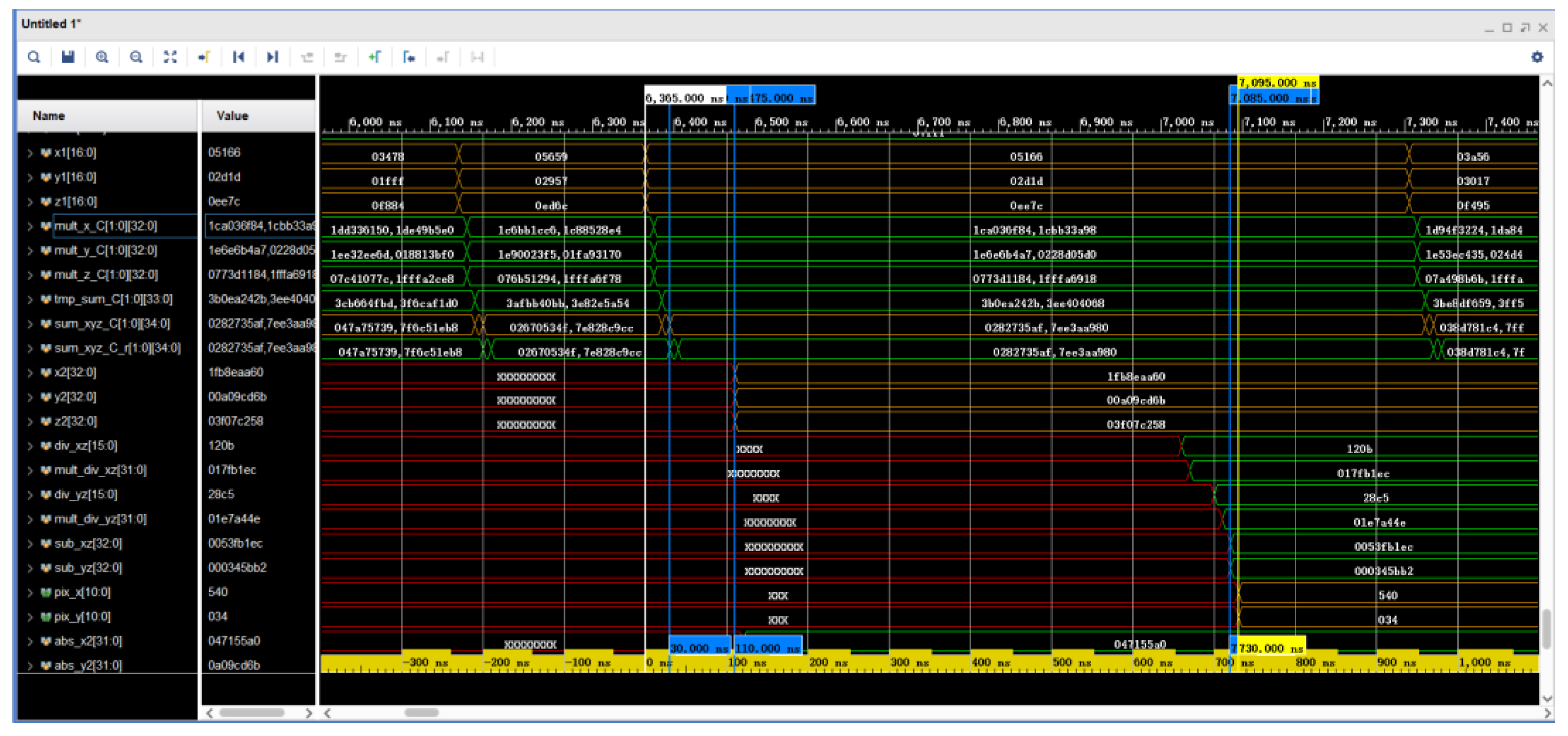
5.7. Simulation Waveform of Star Point Coordinate Transformation

The simulation of the star point space coordinate transformation waveform is shown in Figure 18. The star point space coordinate transformation consists of two parts. The first part is the transformation of the star point coordinates from the celestial coordinate system to the star sensor coordinate system, and the second part is the transformation of the star points in the star sensor coordinate system to the 2D planar coordinate system. ${\left[\begin{array}{ccc}{x}_1& y_1& z_1\end{array}\right]}^T$ are the star point coordinates in the celestial coordinate system, ${\left[\begin{array}{ccc}{x}_2& y_2& z_2\end{array}\right]}^T$ are the star point coordinates in the star sensor coordinates, and pix_x and pix_y are the star point coordinates in the 2D planar coordinate system. Sum_xyz_C are two 32-bit-wide registers that store the star point coordinates and attitude transformation matrix C in the celestial coordinate system. Registers that host the computed results of the star point coordinates and attitude transformation matrix C in the celestial sphere coordinate system. At 6395 ns, the two registers complete the computation simultaneously. At 7085 ns, two adders completed the calculation. The computation process in the figure conforms to the representation of Equations (8), (13) and (14). The FPGA consumes 730 ns for parallel computation here and 770 ns if a fully serial computation method is used.

5.8. Simulation Waveforms of Star Chart Generation

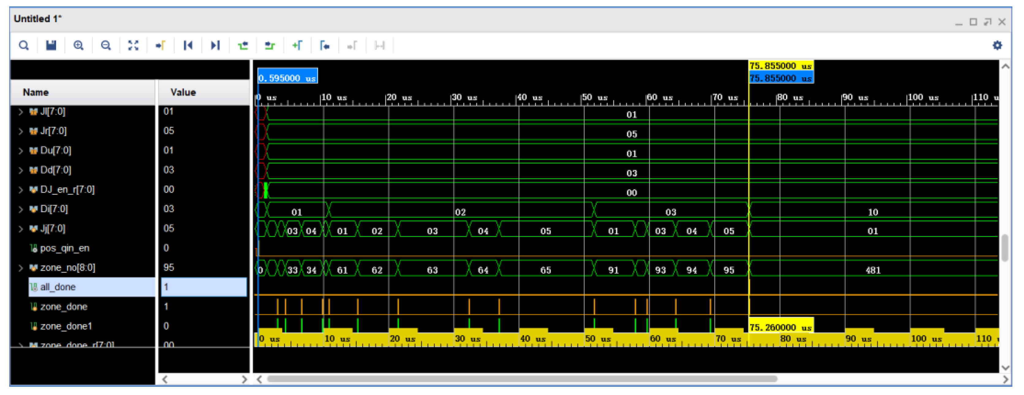
The simulation waveform of target subzone search is shown in Figure 19. In the figure, pos_qin_en is the data input enable signal, zone_no is the current target subzone number, zone_done is the current target subzone search completion signal, and all_done is the whole target subzone search completion signal. It can be observed in the figure that the time from the rising edge of pos_qin_en to the rising edge of all_done is 75.26 μs, which is all the time consumed by the generation of a star map.

In the three parts of optical axis pointing calculation, optical axis pointing coordinate transformation calculation, and star zone search range calculation, a set of attitude quaternions only needs to be calculated once, which takes up a relatively small amount of calculation time. In the three parts of star point coordinate transformation calculation, star point effective judgment, and star point coordinate transformation, every star point data in the subarea range needs to be calculated, and the calculation time takes up a larger proportion. The greater the parallelism of the star point data calculation, the less time consumed by the calculation and the less time consumed by the final star map generation.

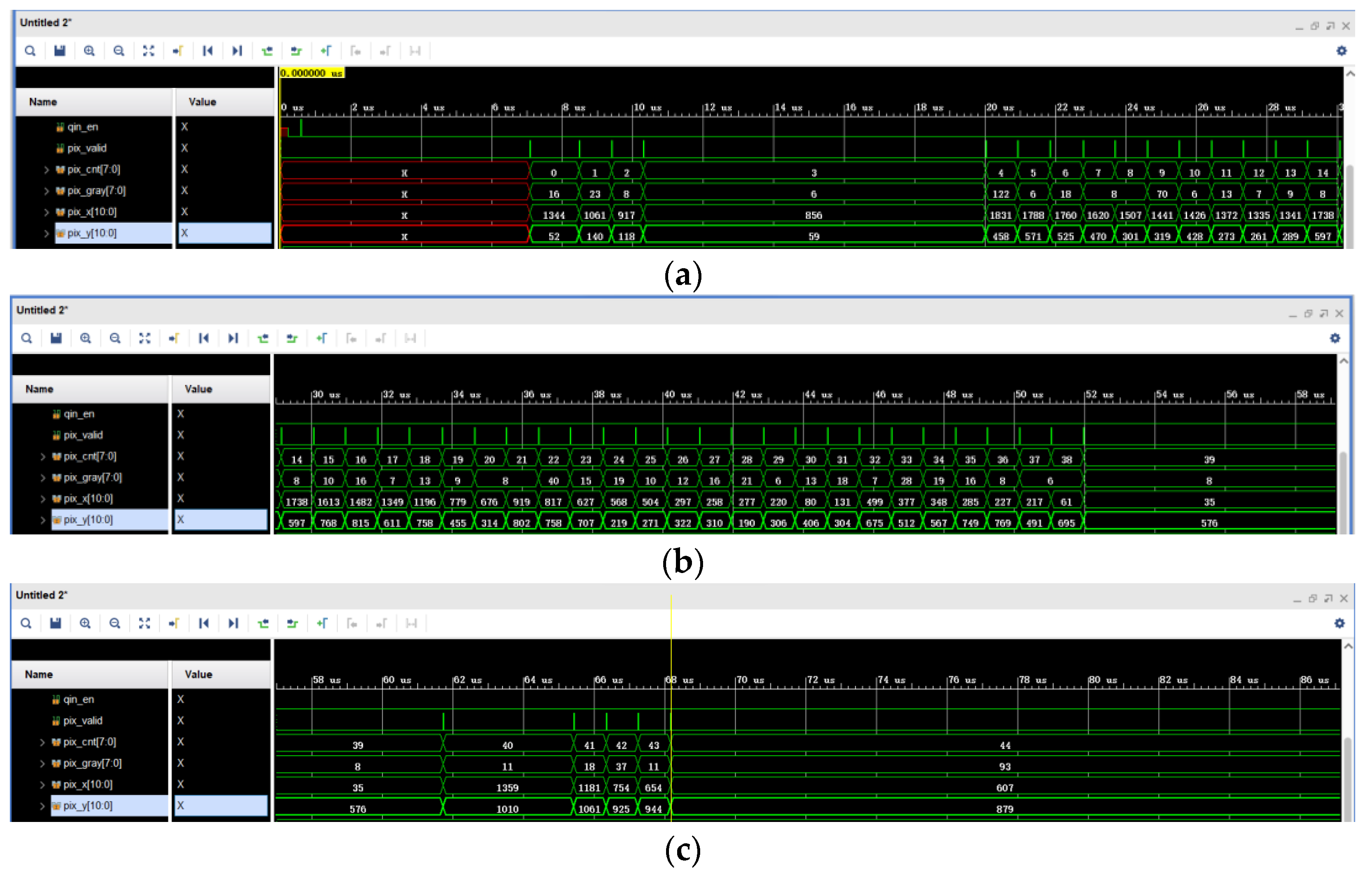
Figure 20 shows the search results of the pixel coordinates and grayscale of the 0th to 44th star points. Moreover, pix_cnt is the effective star points pixel counter, pix_x and pix_y are the horizontal and vertical coordinates of the effective star points pixels, and pix_gray is the grayscale of the effective star points pixels. Based on the results in Figure 20, it can be seen that the computation of the star point pixel coordinates and grayscale values is consistent with the MATLAB calculations in Figure 8 above. Because the number of star points within the search area varies, the star map calculation time varies. The higher the number of star points in the target sub-area, the longer the calculation takes.

5.9. Simulation and Analysis of Dynamic Star Chart Systems

In the three parts of optical axis pointing calculation, optical axis pointing coordinate transformation calculation, and star zone search range calculation, a set of attitude quaternions only needs to be calculated once, consuming a smaller proportion of the total calculation time. In the three parts of star point coordinate transformation calculation, star point effective judgment, and star point coordinate transformation, every star point data in the subarea range needs to be calculated, consuming a larger proportion of the total calculation time. The stronger the parallelism of the star point data calculation, the less time is consumed for calculation, and the less time is consumed for the final star map generation.

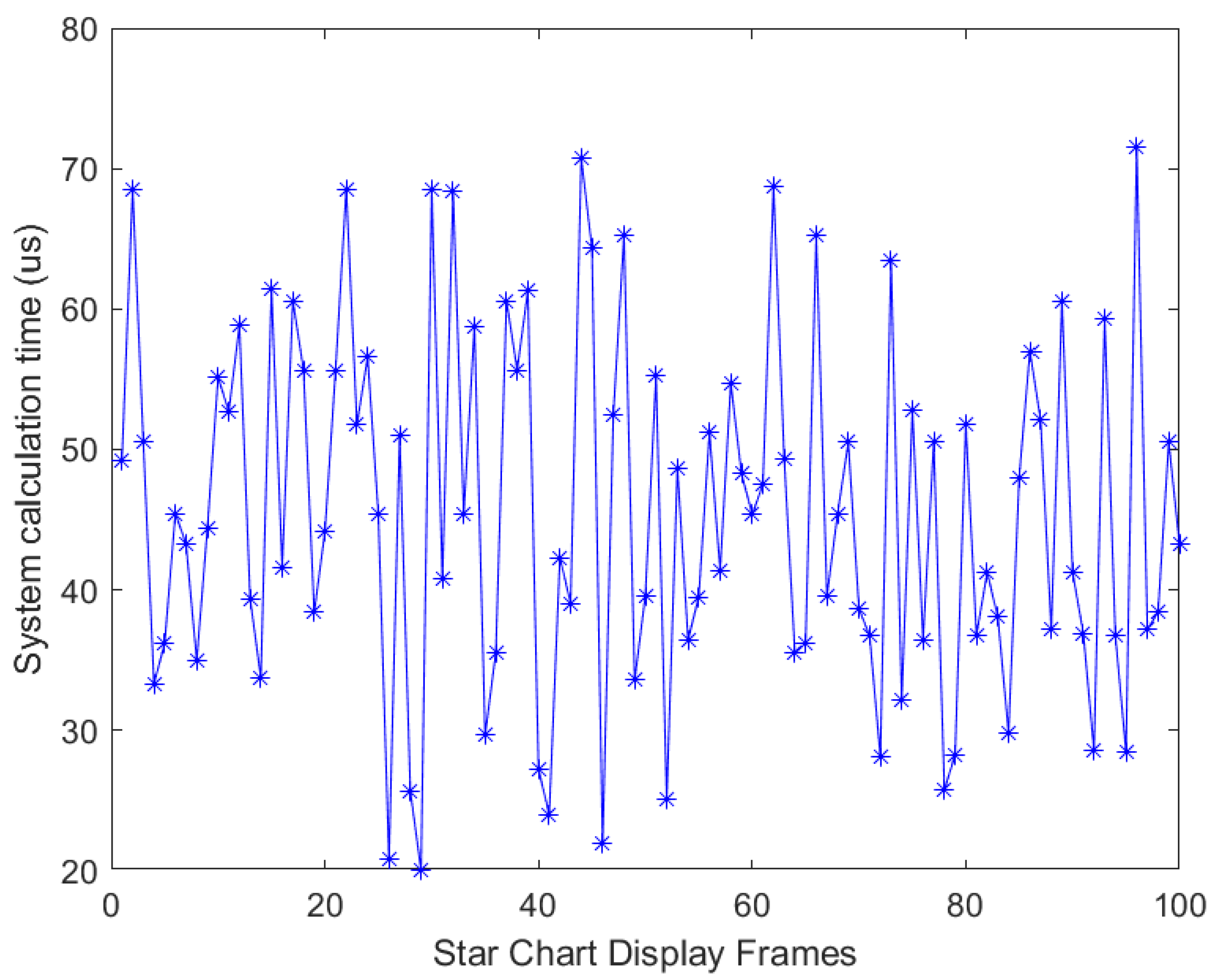
Under the Vivado 2018.3 development environment, 100 sets of attitude quaternions are input randomly in this design to simulate the star chart display algorithm to calculate 100 star charts. As shown in Figure 21, the horizontal coordinate indicates the number of frames of the star charts, and the vertical coordinate represents the time taken by the star chart display algorithm system to compute a star chart. By doing Post-Synthesis Functional Simulation on the project, the experimental schematic of 100 sets of random quaternions at a simulated pixel clock of 148.5 MHz shows that the longest time for the completion of all the sub-area searches is about 72 μs. Compared with the computation time of the current star chart display algorithm of the Dynamic Star Simulator, the computation time of the star chart display algorithm of the present design is about $1/80$ of the former [21].

The number of hardware resources for the FPGA-based dynamic star map algorithm designed in this paper is shown in

Table 4. FPGA hardware resource usage.

Name	Slice LUTs (20,800)	Slice Registers (41,600)	Block RAM Tile (50)	DSPs (90)
project	52.20%	33.14%	8.00%	48.89%
U_sao_top	20.80%	19.26%	0.00%	48.89%
U_sao_zone	6.36%	2.73%	0.00%	32.22%
U_sao_disp	5.37%	4.05%	0.00%	0.00%
U1_div	8.05%	11.52%	0.00%	0.00%
Uart_to_img	0.40%	0.55%	0.00%	0.00%
PLL	0.00%	0.00%	0.00%	0.00%
Dvi_pll	0.00%	0.00%	0.00%	0.00%
Dvi_encoder1	0.89%	0.38%	0.00%	0.00%
Disp_driver	0.25%	0.11%	0.00%	0.00%
DDR3_ctrl_2port	30.16%	12.85%	8.00%	0.00%

. It can be seen that, due to the large number of LUTs used for storing the data streams and the star catalog data, the sub-modules under the computational part of u_sao_top are U_get_zone, U_sao_disp, and U1_div, which use a larger number of DSPs. But there is still a certain amount of margin in the resource usage to complete the subsequent modifications.

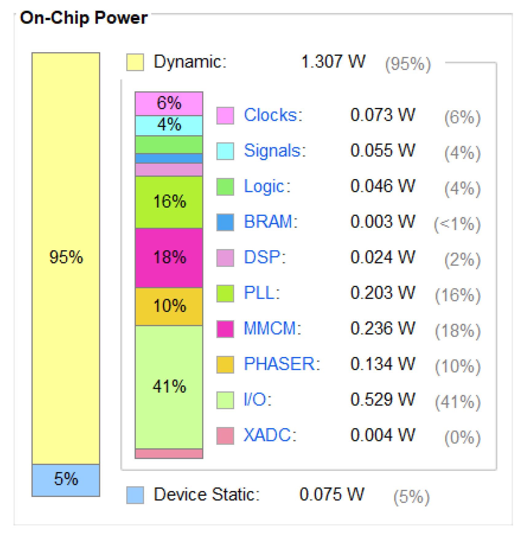
According to the power consumption analysis of Vivado 2018.3, as shown in Figure 22, it can be seen that the dynamic power of this design is 1.307 W, which is significantly lower than the power consumption of using a computer.

Table 5. Comparison of the performance of different methods.

References	Calculation Method	Number of Stars	Computation Time
[5]	serial	9006	56 ms
[6]	serial	15,914	9.43 ms
[7]	serial	5103	7.98 ms
article	parallel	5067	72 μs

shows the comparison of the performance of different methods for star chart computation.

6. Conclusions

In this paper, an FPGA-based algorithm for displaying star charts of a dynamic star simulator is designed that can output star charts under the condition that the star chart field of view is $\mathrm{\Phi }20°$ and the simulated magnitude is $2.0\sim 6.0 \mathrm{Mv}$.

(1) The article analyzes the calculation of the optical axis pointing calculation part, the optical axis pointing coordinate transformation calculation part, the star area search range calculation part, the star point coordinate transformation calculation part, the star point validity judgment part, and the calculation of the star point coordinate transformation part. The article uses the characteristics of FPGA parallel computing with pipelining to improve the calculation speed of data and accelerate the display speed of dynamic star charts.

(2) This design utilizes FPGA to reduce the size and power consumption of the dynamic star simulator, get rid of the dependence of the existing algorithm on the computer, and significantly reduce the star point display time.

Overall, the FPGA-based dynamic star chart algorithm design improves the display speed of star charts. However, there is still room for further optimization of hardware resources, especially the usage of LUTs. At the same time, there are more suitable algorithms for FPGA implementation, which is the direction of the future development of dynamic star map displays.