Abstract
The Delta robot is an over-actuated parallel robot with highly nonlinear kinematics and dynamics. Designing the control for a Delta robot to carry out various operations is a challenging task. Various advanced control algorithms, such as adaptive control, sliding mode control, and model predictive control, have been investigated for trajectory tracking of the Delta robot. However, these control algorithms require a reliable input–output model of the Delta robot. To address this issue, we have created a control-affine neural network model of the Delta robot with stepper motors. This is a completely data-driven model intended for control design consideration and is not derivable from Newton’s law or Lagrange’s equation. The neural networks are trained with randomly sampled data in a sufficiently large workspace. The sliding mode control for trajectory tracking is then designed with the help of the neural network model. Extensive numerical results are obtained to show that the neural network model together with the sliding mode control exhibits outstanding performance, achieving a trajectory tracking error below 5 cm on average for the Delta robot. Future work will include experimental validation of the proposed neural network input–output model for control design for the Delta robot. Furthermore, transfer learnings can be conducted to further refine the neural network input–output model and the sliding mode control when new experimental data become available.
1. Introduction
Delta robots are fast, accurate, and versatile, suitable for tasks like assembly, pick-and-place, sorting, and classification. The Delta robot is a parallel robot with three arms connected to an end effector mounted on its base, exhibiting an over-actuated configuration. Lagrangian dynamics, inverse kinematics, and screw theory are three common approaches to model the Delta robot [1,2,3]. Knowing the dynamic model is essential for motion planning and trajectory tracking. It allows the controller to calculate the required joint inputs to achieve a desired end effector position. The control design of a Delta robot is challenging due to its high level of non-linearity and complicated kinematic and dynamic model. Therefore, plenty of nonlinear and adaptive control algorithms have been implemented for trajectory tracking and disturbance rejection of the Delta robot. Sliding mode control is one of the most popular nonlinear control algorithms [4,5]. This algorithm has been extensively applied to the trajectory tracking of the Delta robot combined with the fuzzy neural network [6], nonlinear proportional-derivative (PD) control [7], and synergetic control [8]. Additionally, Radial Basis Function Neural Networks (RBFNNs) combined with sliding mode control were adopted in [8,9] to compensate for the unknown disturbances. The work reported in [10] proposed an online estimation approach to compensate for various uncertainties in the Delta robot and to improve the tracking performance. An adaptive active disturbance rejection control was adopted for the output-based robust trajectory tracking of the Delta robot in [11]. Iterative learning control has also been applied to the trajectory tracking of the Delta robot with a high performance. Boundjedir, C.E. and Bouri, M. [12] proposed a PD-type ILC combined with PD control to improve the iteration performance. Model-free iterative learning control was further implemented on the Delta robot with non-repetitive trajectories [13]. Moreover, a model reference adaptive control has also been adopted for control of the Delta robot. Combining an identified linear model with mode reference adaptive control has shown a significant performance improvement compared to the three commonly used methods: PID, adaptive control, and sliding mode control algorithms [14].
Besides traditional control algorithms, neural networks were also adopted to improve the trajectory-tracking performance of the Delta robot. An inverse kinematic controller using neural networks was presented in [15] for trajectory control of a Delta robot in real-time by making use of data collected from simulation. Ref. [16] proposed a data-driven optimal control algorithm by approximating the solution of the Hamilton–Jacobi–Bellman equation using neural networks. A neural network model was proposed in [17] to approximate the inverse kinematics of the Delta robot with randomly sampled experimental data and was implemented on the hardware in an open-loop control for trajectory tracking.
Most of the advanced control algorithms mentioned above are either data-driven or model-based. Model-based control algorithms are highly dependent on the accuracy of the model. Therefore, they have high requirements for control robustness in terms of model uncertainties and disturbances. On the other hand, data-driven algorithms operate independent of model accuracy requirements. Given the paramount importance to safety considerations during normal operations, ensuring robustness and maintaining optimal performance pose significant challenges in the control design of Delta robots employing data-driven algorithms. Moreover, another challenge in Delta robot control is the singularity [18,19], which occurs when the end effector is positioned at specific locations where the kinematic model degenerates and the joint angles become indeterminate, which can lead to erratic behavior and potential damage to the robot. Therefore, understanding the robot’s geometry and workspace is crucial to avoid singularities, which can cause significant problems during operation.
In this study, we consider a Delta robot equipped with stepper motors as inputs. Once the desired trajectory of the end effector is determined, inverse kinematics can be adopted to solve for the joint inputs analytically or numerically using optimization methods. Moreover, control algorithms can be implemented to further improve the reliability of the motion and the trajectory tracking accuracy of the Delta robot. The objective of this study is to develop a hybrid of data-driven and model-based sliding mode control algorithms instead of using the conventional optimal control to improve the trajectory tracking performance. The inverse kinematics of the Delta robot is analytically difficult to express in the control-affine form, which complicates the control design process. Therefore, to deal with this issue, we propose that neural networks are used to create a control-affine nonlinear input–output dynamic model of the Delta robot, considering the stepper motor angles and velocities as inputs. The neural network input–output model is trained with randomly sampled data in a sufficiently large workspace of the Delta robot. Furthermore, the model-based sliding mode control for trajectory tracking is designed based on the neural network model. The proposed neural networks make full use of the inverse kinematics while the sliding mode control delivers excellent performance in trajectory tracking for a Delta robot. We should point out that the proposed control-affine nonlinear dynamic model of the Delta robot is not derivable either from Lagrangian dynamics or inverse kinematics. It is completely data-driven and can be updated once new experimental data become available. This is also one of the contributions from our work.
Section 2 presents the architecture of the Delta robot and its inverse kinematics. Section 3 presents the control-affine nonlinear dynamic model in terms of the neural networks. Section 4 presents the sliding mode control with the neural network model and extensive numerical simulation results to validate the proposed model and control design. Section 5 concludes this paper.
2. Dynamic Model of Delta Robot
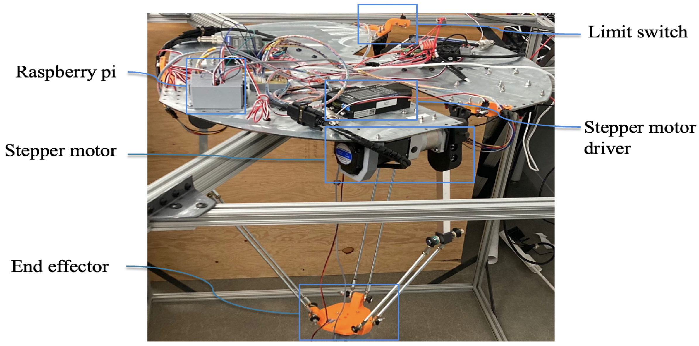
The mechanical structure of a three-DOF Delta robot is shown in Figure 1. Figure 2 shows the geometry and coordinates of the Delta robot in 2D and 3D views. A typical Delta robot is composed of a fixed platform, a moving platform, three active arms, and three passive arms connected to an end effector mounted on the base. The active arms of the robot are driven by the rotation actuators, which are stepper motors in this study. The parameters of the Delta robot are given in Table 1, and the specifications of components used for fabricating the Delta robot can be found in [17].
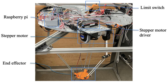
Figure 1.
Hardware setup of the Delta robot.
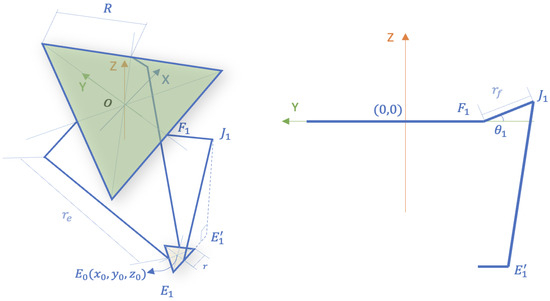
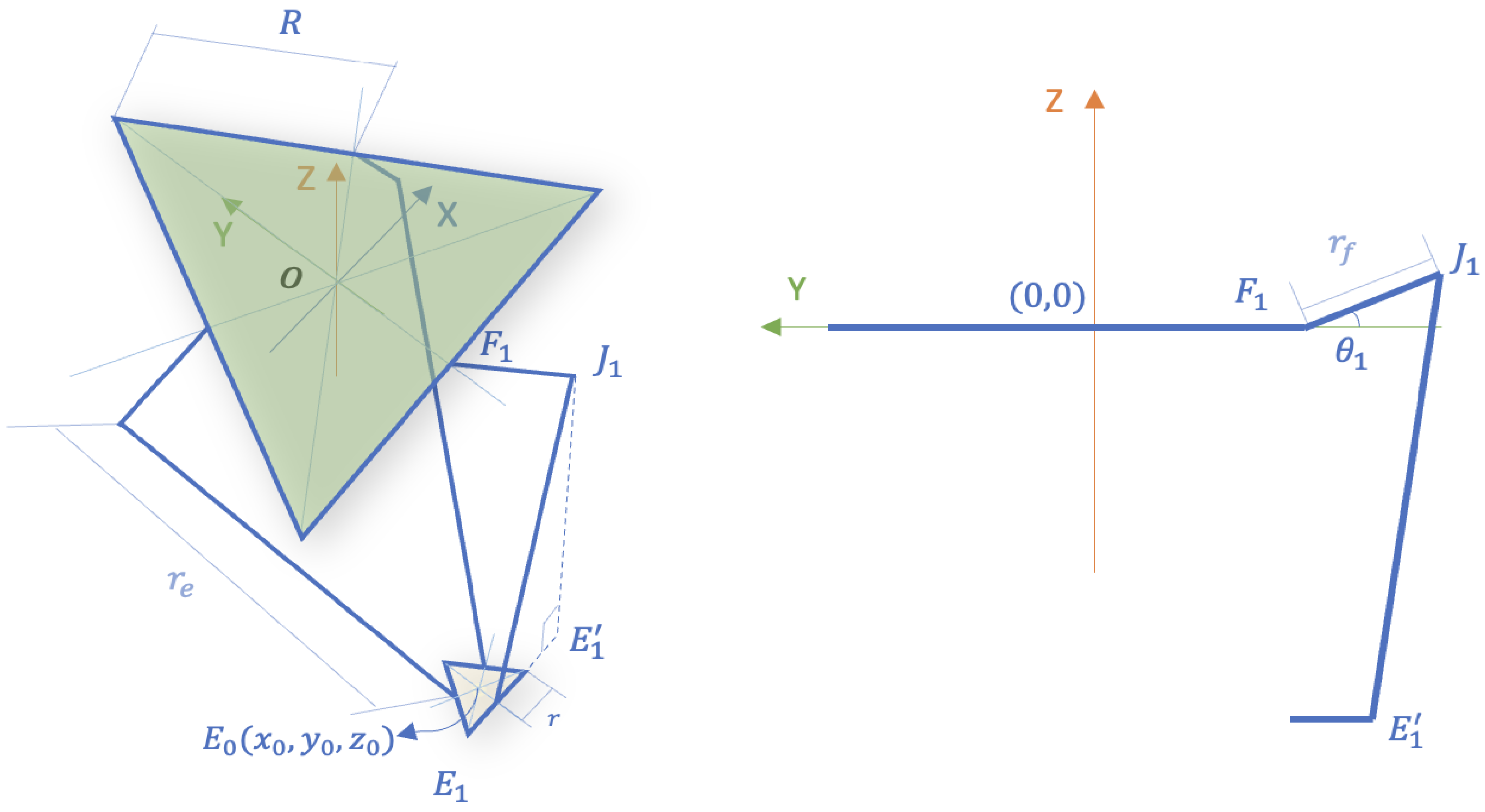
Figure 2.
The geometric configuration and coordinate framework required to model the inverse kinematics of the Delta robot. Left: geometric structure of the Delta robot in 3D. Right: two-dimensional projection of geometry and coordinates of the Delta robot joints and links.

Table 1.
Parameters of the Delta robot.
Inverse Kinematics
Inverse kinematics stands out as one of the most widely adopted algorithms for modeling the Delta robot. Solving the inverse kinematics involves deriving the geometrical relationships between its links and joints. From Figure 2, the relationship between the link positions and angles can be given as
where ; and are the positions of the points and in the Y direction; and and are the positions of the points and in the Z direction. The positions of the joints and satisfy the geometric constraints of the Delta robot as described in [17].
The inverse kinematics describes how the angles of the joints relate to the positions of the end effector. The joint velocities are not considered in Equation (1). In this study, the control inputs include angles and joint velocities of the stepper motors. Hence, the dynamic input–output model of the Delta robot should involve joint velocities. One way to compute the joint velocities is by using the Jacobian matrix J that relates to the joint velocities and the end effector position velocities [20]:
where describes the centroid position of the end effector. Equations (1) and (2) suggest that the joint velocities are highly nonlinear and complex functions of the positions and its velocities of the end effector. In the data-driven study, the joint velocities can be computed using finite difference approximation as, for example,
where k is the discrete time, i represents the stepper motor’s index number and is the sample time. However, as discussed in the Section 1, this information alone is not enough to help us build a dynamic input–output model for the Delta robot. Furthermore, if the finite difference method or Jacobian matrix method is used to compute joint velocities, errors in the computed velocities can accumulate over time, leading to a poor position prediction. This affects the performance of trajectory tracking control.
It is commonly known that the control-affine model of a system provides a convenient platform for control design. In this study, we propose to develop a control-affine nonlinear model of the Delta robot by utilizing neural networks. Neural networks can learn and model the underlying physical relationship between the inputs and outputs. A rich set of input–output data from the forward model of the Delta robot can be used to train neural networks in order to build the control-affine nonlinear dynamic model of the Delta robot without the need for the Jacobian matrix, finite difference, and inverse kinematics. The proposed control-affine model is completely data-driven and is intended for control design consideration. The model is not derivable from Newton’s law or Lagrange’s equation. The input–output data for training the neural networks are randomly sampled in a sufficiently large workspace. Moreover, the neural network model can be further updated by incorporating the concept of transfer learning when new experimental data become available.
3. Neural Network Model
The nonlinear control-affine model with stepper motor joint angles and velocities as inputs makes the control design relatively straightforward and is given in the following.
where , , , and are nonlinear functions of their arguments, and , , and represent the position of the end effector at the centroid along the x, y, and z axes.
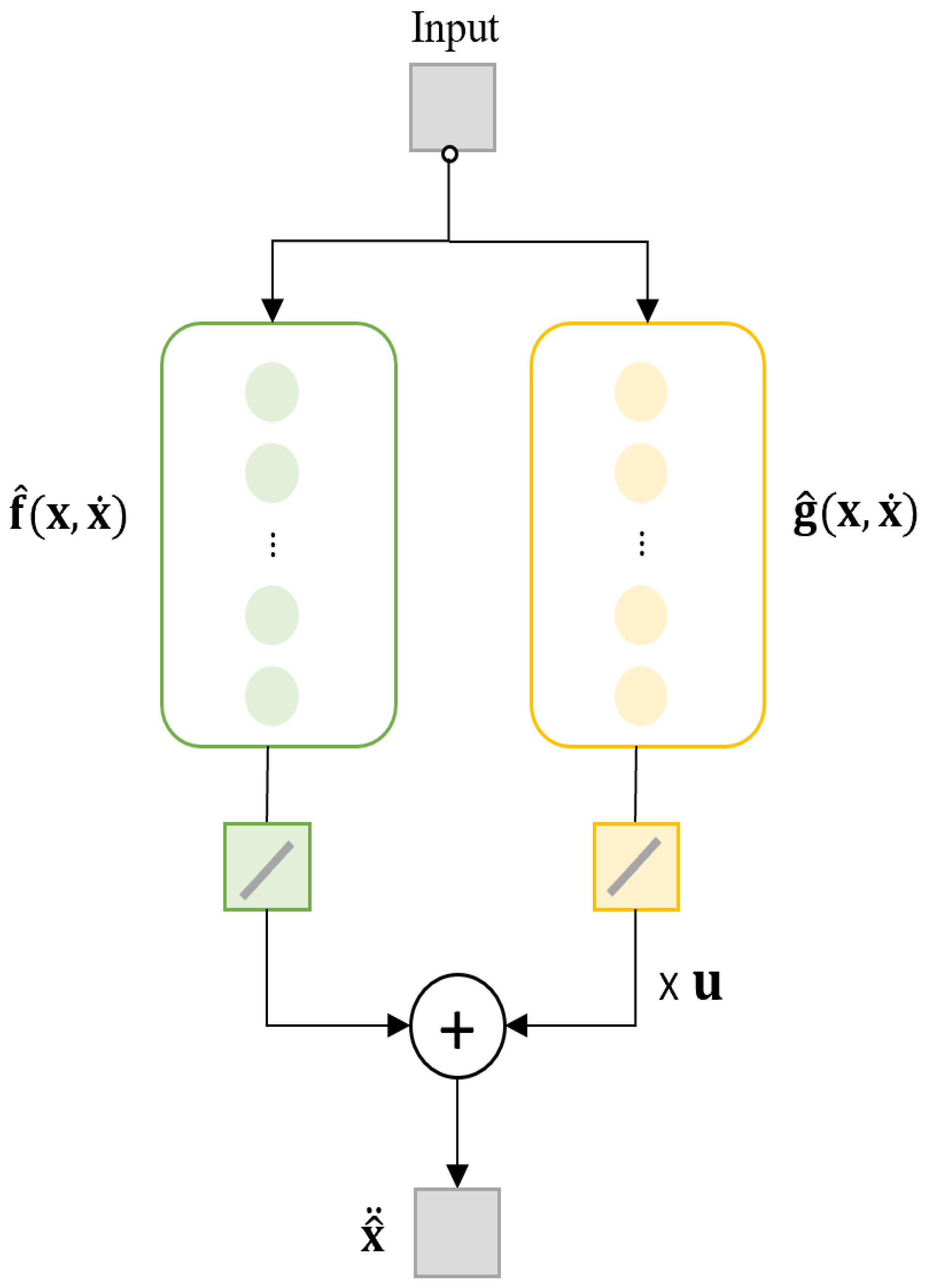
As pointed out before, the control-affine form of the model is not directly derivable from Newton’s law, Lagrangian dynamics, or inverse kinematics. Although various dynamic models for the Delta robot that use the computed-torque approach are available in the literature, they cannot be applied to this study, since the inputs of the Delta robot are only the joint angles and velocities. Here, the neural networks are adopted to approximate the nonlinear functions of the dynamic model for the Delta robot. Specifically, two neural networks are constructed to approximate the nonlinear functions and . Notably, with an extra hidden layer and an additional input, a single neural network can be customized to approximate the two nonlinear functions. The structure of the proposed neural network model for the Delta robot is shown in Figure 3.
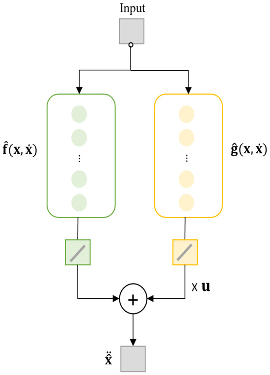
Figure 3.
A flowchart illustrating the neural network model of the Delta robot.
The inputs for neural networks are , , and . The output for the neural networks is , which can be expressed in terms of the two neural networks and :
where n is the sample time. The loss function is defined as
where is the prediction from neural networks and is the system response. Data can be collected from simulations or experiments, and is the total number of sampled points.
Detailed information of the number of hidden layers, type of activation function, and number of neurons are shown in Table 2. Here, the sigmoid neuron is chosen as the activation function. Other activation functions such as tanh or ReLU can also be considered based on the universal approximation theorem of neural networks. The number of training epochs is set as 20,000. The chosen optimization algorithm is stochastic gradient descent (SGD). Dropout with a frequency of 0.5 is adopted to prevent overfitting. The SGD algorithm is one of the most popular stochastic optimization methods in the machine learning community [21]. In this study, it has been adopted as the optimization algorithm to train the neural networks. The stochastic gradient descent maintains a single learning rate to update all weights compared to Adam [22]. The loss value reached 0.000281 after training for 20,000 epochs.
Table 2.
Summary of neural networks.
A remark on the choices of various hyper-parameters for the neural networks is in order. We have to say that the parameters we used are not guaranteed to be optimal. Since there is no established general rule for selecting the hyper-parameters of neural networks, some level of trial and error is involved with specific data set of different applications.
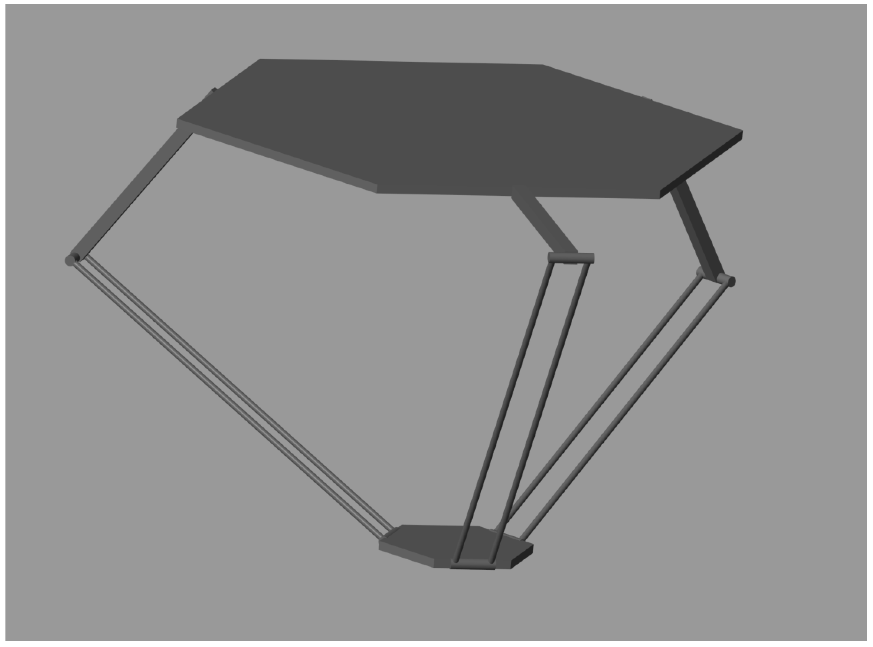
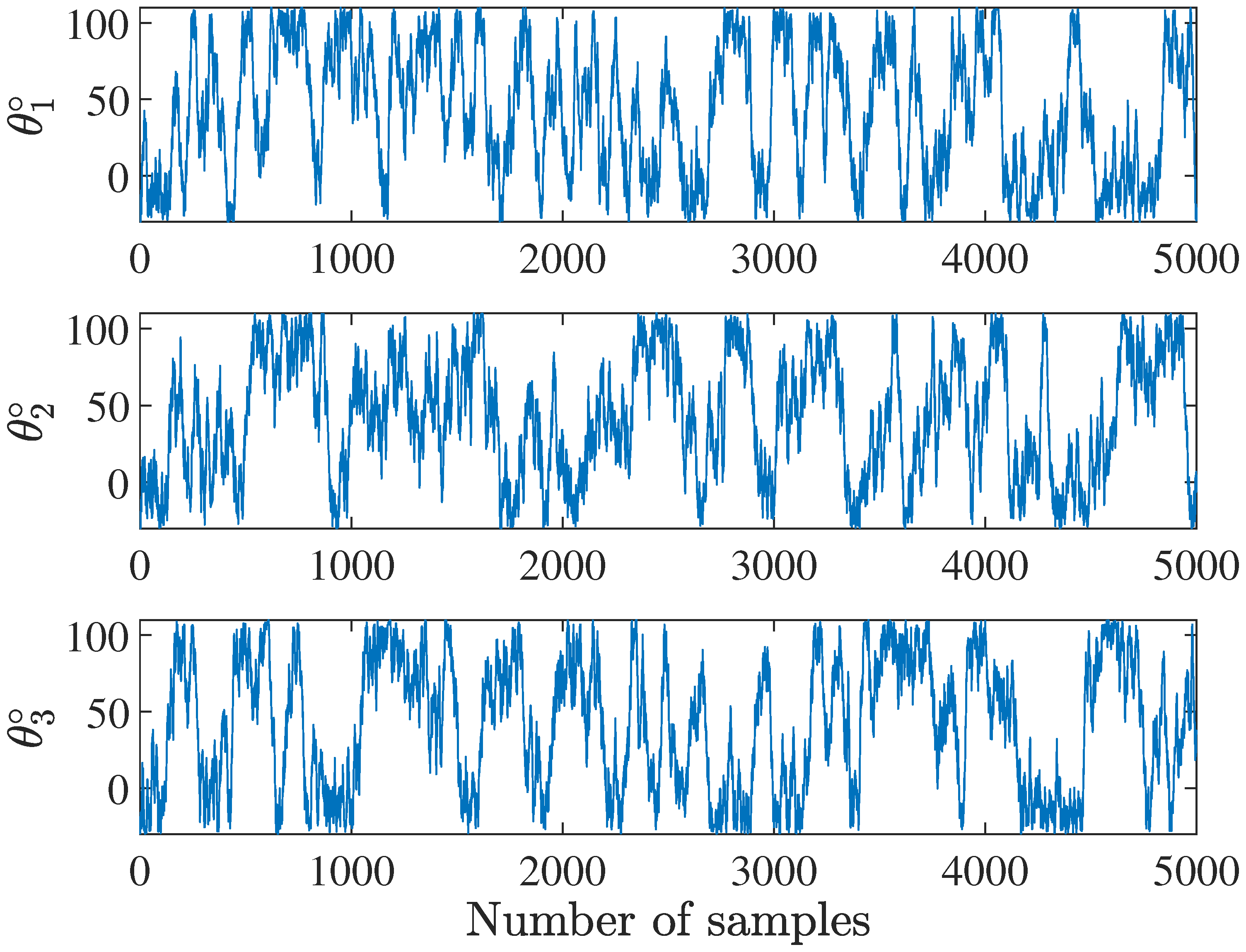
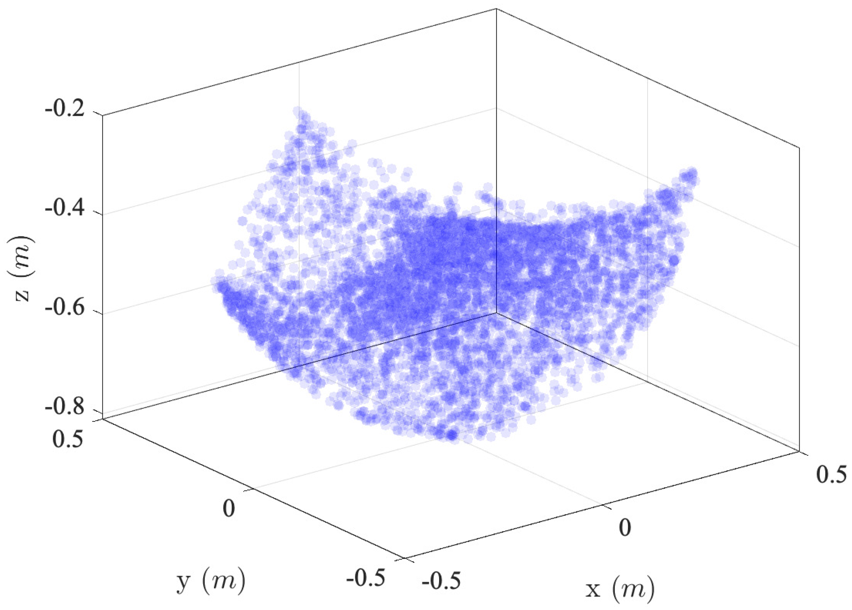
With the help of the dynamic model built in Section 2, a SimScape model of the Delta robot is developed and used to generate the data of time series and . The SimScape model of the Delta robot is shown in Figure 4 and created based on the actual Delta robot that is to be used for the experiment, as shown in Figure 1 and Table 1. The parameters of this modeled Delta robot are digital twins of those listed in Table 1. To generate training data, we randomly sample joint angles in a bounded range of , as shown in Figure 5, in order to cover the typical workspace of the Delta robot. A total of 2500 data points are sampled in the workspace, and 75% of the data are chosen as training data set, and 25% of the data are chosen as validation data set. The corresponding positions of the end effector in 3D are shown in Figure 6. The boundary of these points is associated with the maximum of the positions in the workspace of the end effector of the targeted Delta robot.

Figure 4.
SimScape model of Delta robot.
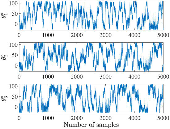
Figure 5.
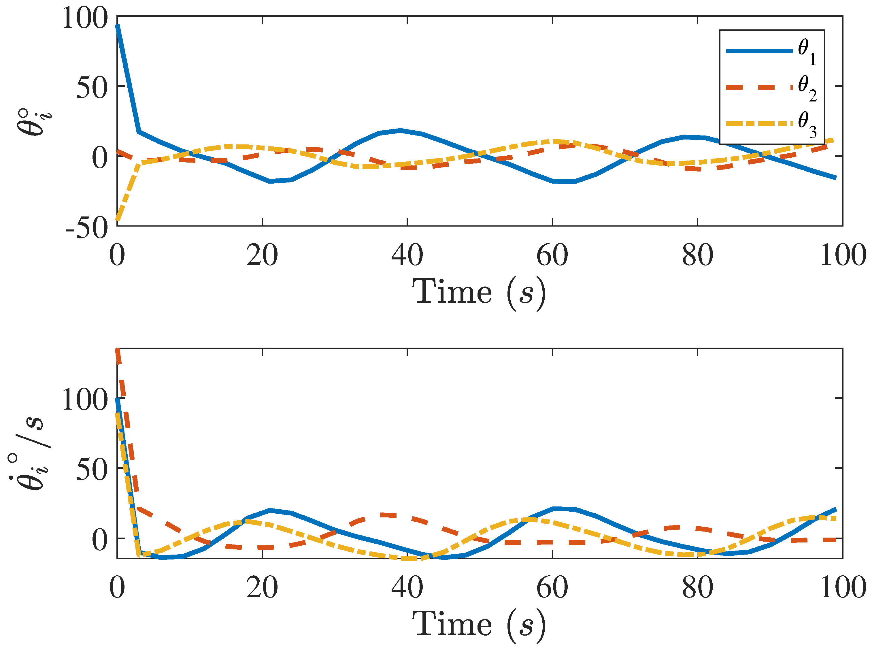
Random joint angles for SimScape Delta robot model. Top: joint angle for stepper motor 1. Middle: joint angle for stepper motor 2. Bottom: joint angle for stepper motor 3.
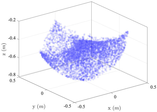
Figure 6.
Random sampled points in the 3D workspace of the Delta robot.
4. Sliding Mode Control
Recall the control-affine nonlinear model in terms of the neural networks in Equation (5). We have
Assume that the Delta robot will track the desired trajectory . The tracking error and its derivative are given as
We select a sliding surface as
where is positive-definite and satisfies the Hurwitz stability condition. Thus, the sliding mode control can be designed as [23]
where and are constant gains, and . Chattering is a prevalent concern associated with sliding mode controllers with switching term . To reduce the chattering in the sliding mode control, the switching terms for the control law and the sliding surface have to be carefully chosen [24]. In this paper, the continuous function is adopted to replace the discontinuous sign function [25]. determines the steepness of as an approximation of the sign function. To prove the stability of the sliding mode control, we shall need the following lemma.
Lemma 1.
Let , then , implies that [26]
Define a Lyapunov function as
Then, we have
Since
therefore, we obtain
Hence, the closed-loop system is stable. Furthermore, we have
According to Lemma 1, we conclude that exponentially decreases at the rate when is outside the boundary layer defined by , and at the rate of when is located inside the boundary layer. In both cases, we have
Hence, the tracking error of the sliding mode control for the system in Equation (7) converges asymptotically to zero at the exponential rate. On the other hand, when the neural network model of the Delta robot has a sufficiently small error, it can be expected that the sliding mode control will deliver similar tracking performance in experiments. This is a subject of on-going work. In this paper, we applied neural network model-based sliding mode control to the physics- and geometry-based model of the Delta robot, and carried out numerical simulations to observe and evaluate the validity of the proposed neural network modeling and control design approach.
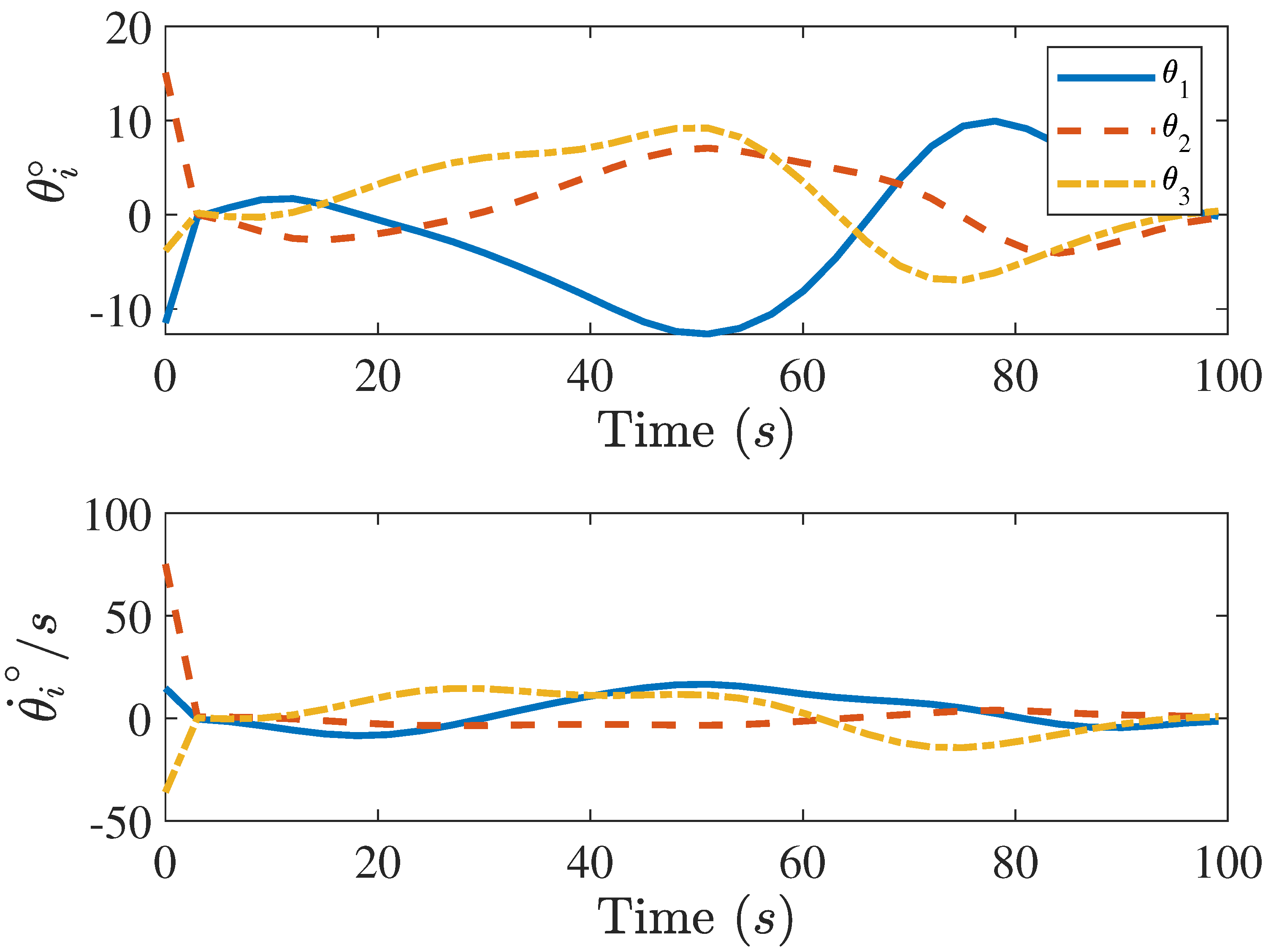
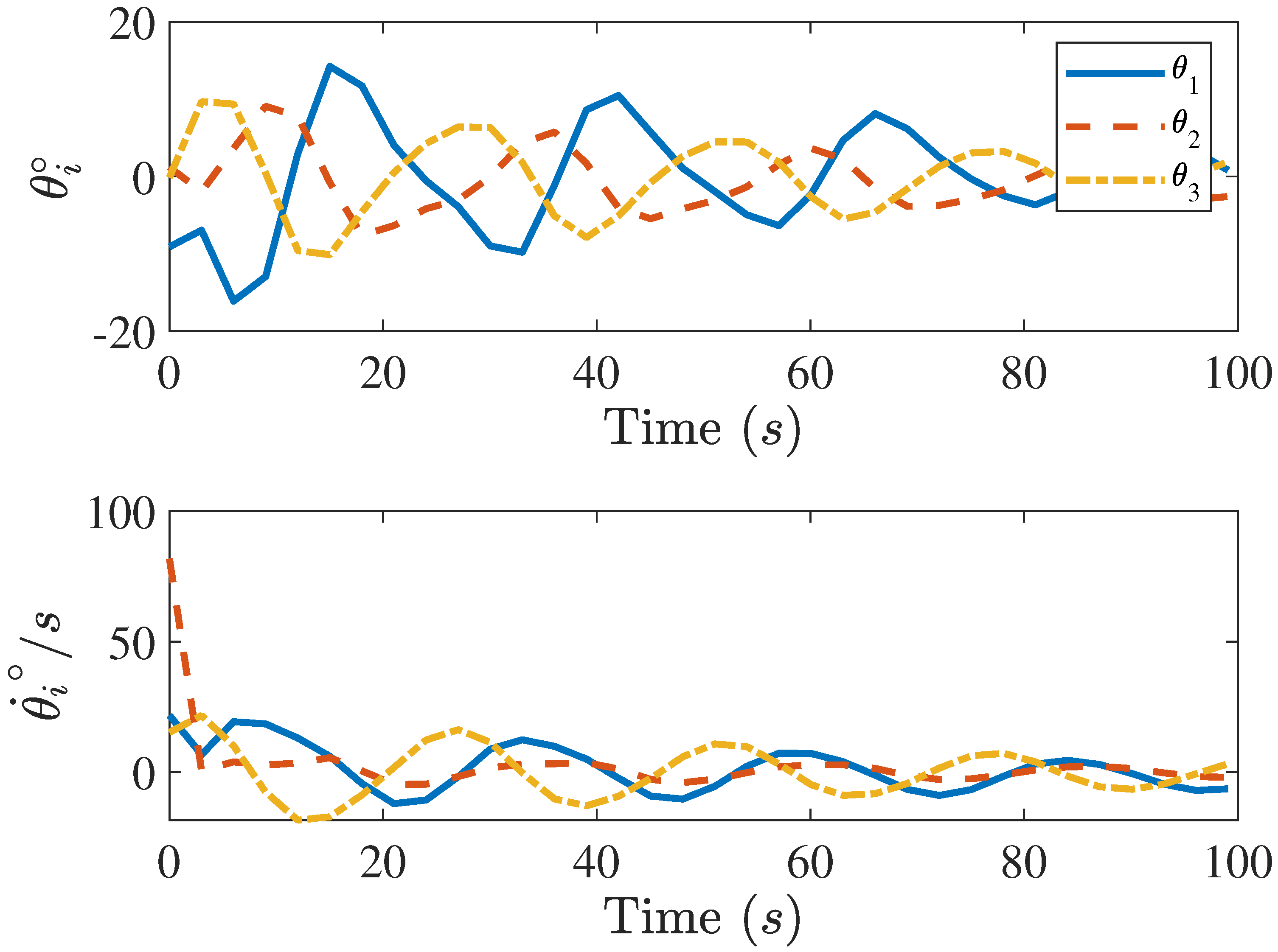
In the following examples, we take as where is the identity matrix, , , and . Three different paths are adopted to test the performance of the proposed sliding mode control. The mathematical expressions of three paths, namely heart curve, logarithmic spiral, and spiral, are given as follows.
where is the end of the time. The 3D tracking results and part of the control inputs for different paths are shown in Figure 7, Figure 8, Figure 9, Figure 10, Figure 11 and Figure 12. The neural network model-based sliding mode control demonstrates remarkable performance in trajectory tracking of various paths while maintaining bounded control inputs. This indicates that the trained neural network model successfully captures the Delta robot’s nonlinear property with an acceptable magnitude of tracking error. The trajectory tracking errors of the sliding mode control for different curves are shown in Figure 13. The initial conditions for the tracking of all trajectories are chosen as .
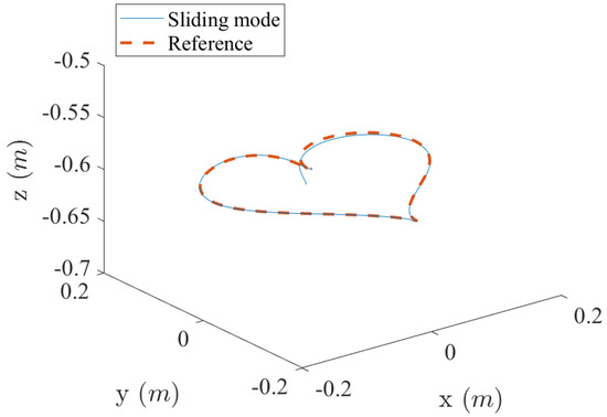
Figure 7.
Three-dimensional trajectory tracking of heart curve using the sliding mode control with the neural network control-affine model.
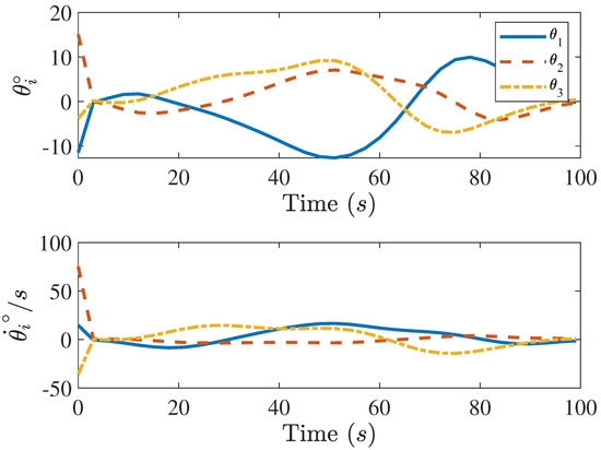
Figure 8.
Magnitude of the sliding mode control with the neural network control-affine model for heart curve trajectory tracking.
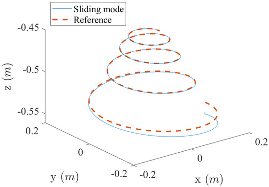
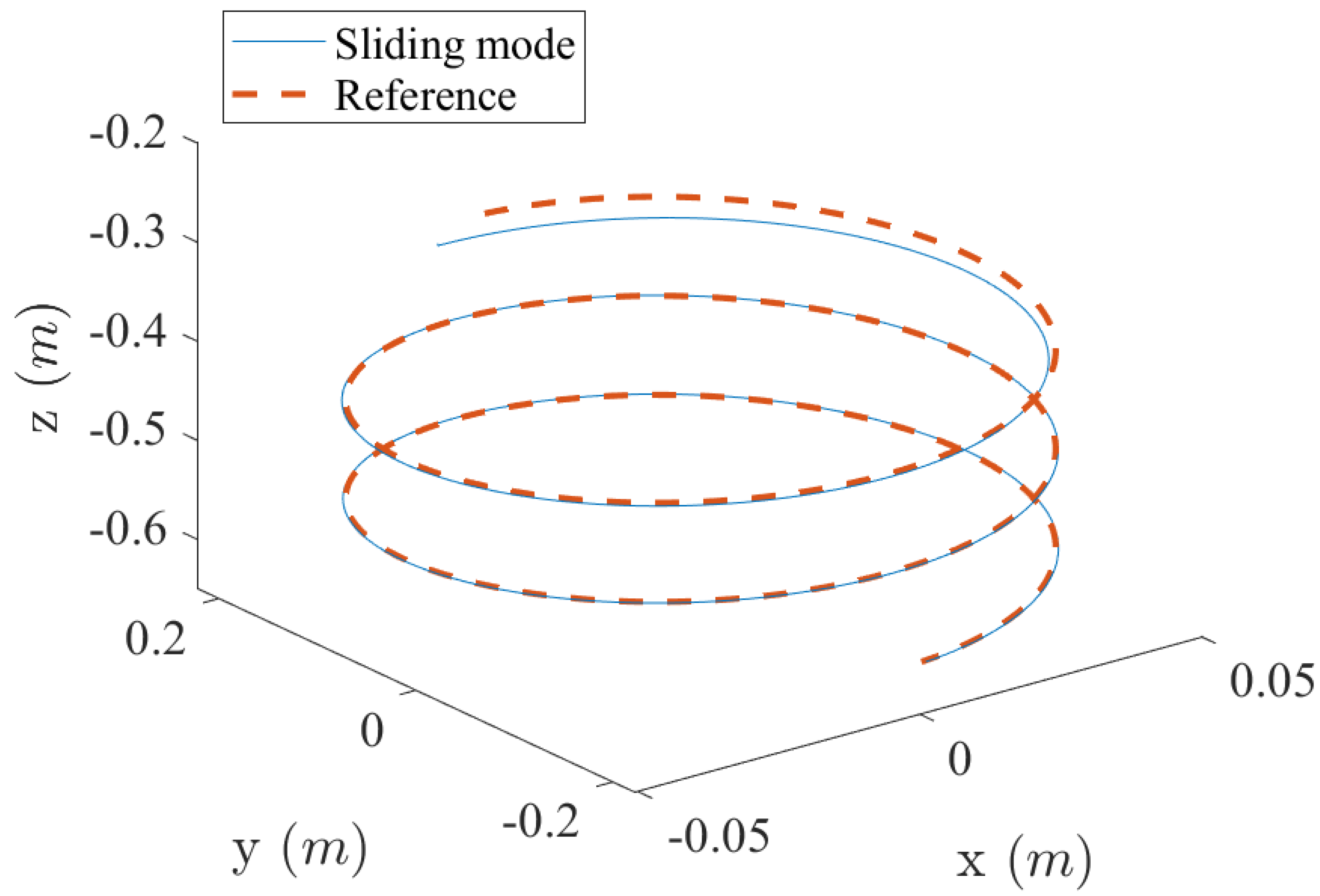
Figure 9.
Three-dimensional trajectory tracking of logarithmic spiral curve using the sliding mode control with the neural network control-affine model.

Figure 10.
Magnitude of the sliding mode control with the neural network control-affine model for logarithmic spiral curve trajectory tracking.
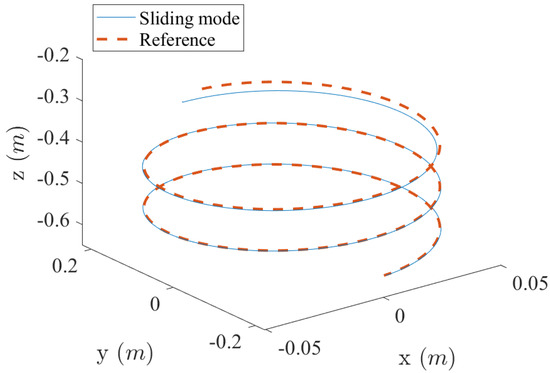
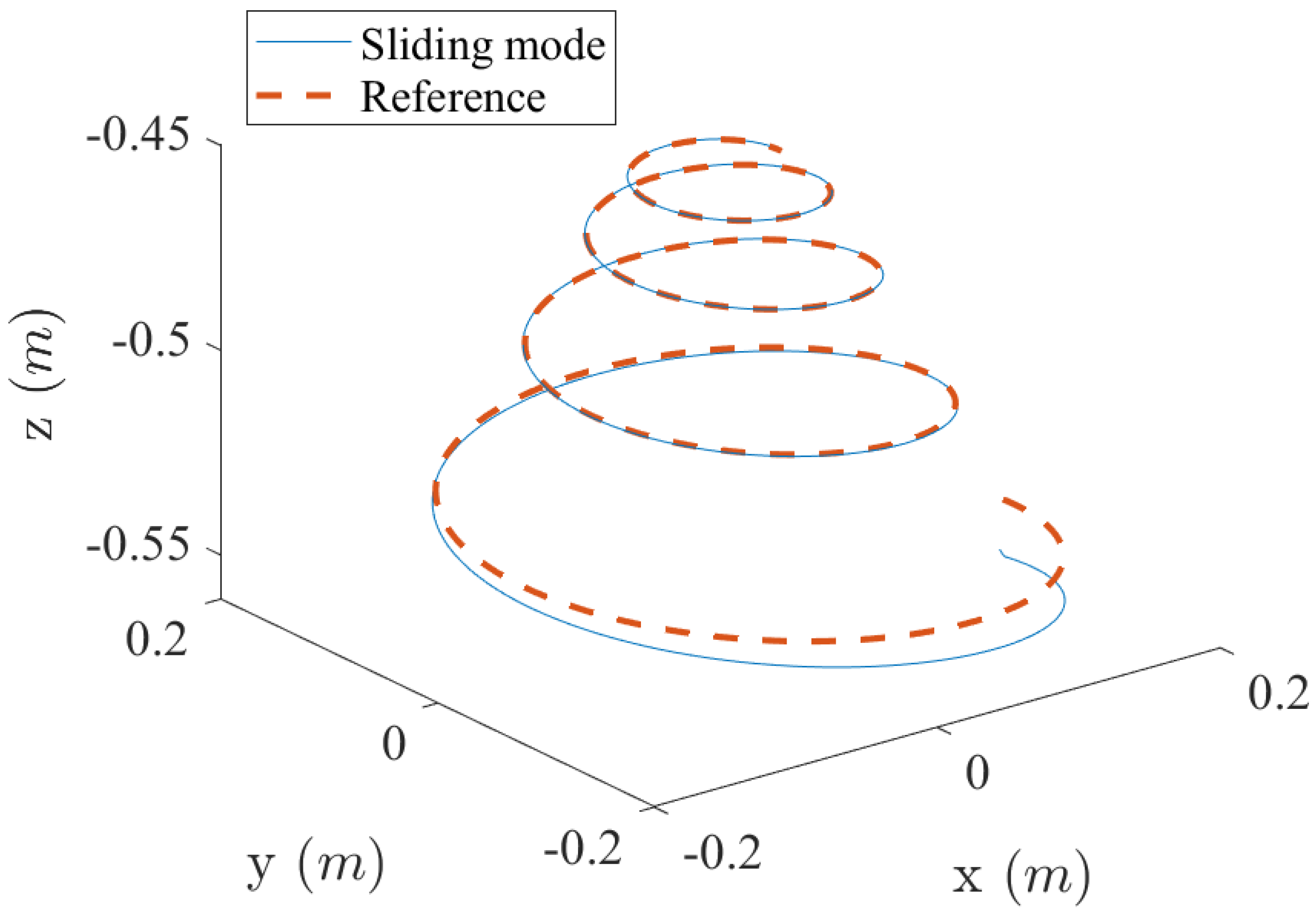
Figure 11.
Three-dimensional trajectory tracking of spiral curve using the sliding mode control with the neural network control-affine model.

Figure 12.
Magnitude of the sliding mode control with the neural network control-affine model for spiral curve trajectory tracking.
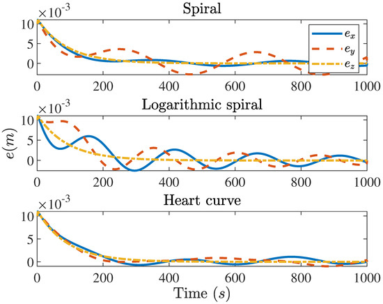
Figure 13.
Tracking error of the sliding mode control in Equation (8) for different curves. Up: the error for spiral trajectory tracking. Middle: the error for logarithmic spiral trajectory tracking. Bottom: the error for heart curve trajectory tracking.
A detailed summary of the trajectory tracking errors are shown in Table 3. By evaluating these results, it is found that the maximum value of tracking error for different curves are the same, and the trajectory tracking errors all converge to zero in a finite time.
Table 3.
Summary of different trajectory tracking errors in m.
5. Conclusions
Delta robots have highly nonlinear dynamics. Finding a control-affine model to describe the input–output relationship of the Delta robot analytically with joint angles and velocities as inputs is difficult. Since it is difficult to obtain the analytical representation of the input–output model, a neural network representation was developed to represent the model. This is a completely data-driven model intended for control design consideration, and it is not derivable from Newton’s law or Lagrange’s equation. The neural networks are trained with randomly sampled data in a sufficiently large workspace. Then, the sliding mode control is designed by making use of the control-affine model to track the desired trajectory. Extensive numerical results have shown that the neural network model-based sliding mode control can be highly effective for trajectory tracking for paths with varying complexity. However, in real-world applications, this control approach can be challenging due to differences in parameters of the frames, arms, and joints, as well as the presence of backlash and flexibility in the joints of the Delta robot. These factors can affect the implementation of neural network-based sliding mode control on hardware. Moreover, the parameters of the sliding mode control need to be fine-tuned based on the specific hardware being used, and high-frequency data collection is required for successful implementation. To overcome these challenges, further work is required to implement neural network-based sliding mode control on hardware. With real data collected from experiments, the method of transfer learning can be applied to refine the neural network input–output model and to update the parameters of the sliding mode control.
Author Contributions
Conceptualization, A.Z. and J.-Q.S.; methodology, A.Z. and J.-Q.S.; software, A.Z.; hardware, A.T. and A.Z.; writing—original draft preparation, A.Z.; writing—review and editing, A.Z., A.T., R.E. and J.-Q.S.; supervision, R.E., J.H.V. and J.-Q.S. All authors have read and agreed to the published version of the manuscript.
Funding
This research was funded by the AI Research Institutes program supported by NSF and USDA-NIFA under the AI Institute: Agricultural AI for Transforming Workforce and Decision Support (AgAID) award No. 2021-67021-35344.
Data Availability Statement
Data are contained within the article.
Conflicts of Interest
The authors declare no conflicts of interest.
References
- Angel, L.; Viola, J. Fractional order PID for tracking control of a parallel robotic manipulator type delta. ISA Trans. 2018, 79, 172–188. [Google Scholar] [CrossRef] [PubMed]
- Zubizarreta, A.; Larrea, M.; Irigoyen, E.; Cabanes, I.; Portillo, E. Real time direct kinematic problem computation of the 3PRS robot using neural networks. Neurocomputing 2018, 271, 104–114. [Google Scholar] [CrossRef]
- Abed Azad, F.; Ansari Rad, S.; Hairi Yazdi, M.R.; Tale Masouleh, M.; Kalhor, A. Dynamics analysis, offline-online tuning and identification of base inertia parameters for the 3-DOF Delta parallel robot under insufficient excitations. Meccanica 2022, 57, 473–506. [Google Scholar] [CrossRef]
- Utkin, V.I. Sliding mode control design principles and applications to electric drives. IEEE Trans. Ind. Electron. 1993, 40, 23–36. [Google Scholar] [CrossRef]
- Perruquetti, W.; Barbot, J.P. Sliding Mode Control in Engineering; CRC Press: Boca Raton, FL, USA, 2002. [Google Scholar]
- Xu, J.; Wang, Q.; Lin, Q. Parallel robot with fuzzy neural network sliding mode control. Adv. Mech. Eng. 2018, 10, 1687814018801261. [Google Scholar] [CrossRef]
- Boudjedir, C.E.; Boukhetala, D.; Bouri, M. Nonlinear PD plus sliding mode control with application to a parallel Delta robot. J. Electr.-Eng.-Elektrotechnicky Cas. 2018, 69, 329–336. [Google Scholar] [CrossRef]
- Pham, P.C.; Kuo, Y.L. Robust adaptive finite-time synergetic tracking control of Delta robot based on radial basis function neural networks. Appl. Sci. 2022, 12, 10861. [Google Scholar] [CrossRef]
- Yen, V.T.; Nan, W.Y.; Van Cuong, P. Robust adaptive sliding mode neural networks control for industrial robot manipulators. Int. J. Control. Autom. Syst. 2019, 17, 783–792. [Google Scholar] [CrossRef]
- Zhao, R.; Wu, L.; Chen, Y.H. Robust control for nonlinear Delta parallel robot with uncertainty: An online estimation approach. IEEE Access 2020, 8, 97604–97617. [Google Scholar] [CrossRef]
- Castañeda, L.A.; Luviano-Juárez, A.; Chairez, I. Robust trajectory tracking of a Delta robot through adaptive active disturbance rejection control. IEEE Trans. Control Syst. Technol. 2014, 23, 1387–1398. [Google Scholar] [CrossRef]
- Boudjedir, C.E.; Bouri, M.; Boukhetala, D. Iterative learning control for trajectory tracking of a parallel Delta robot. At-Autom. 2019, 67, 145–156. [Google Scholar] [CrossRef]
- Boudjedir, C.E.; Bouri, M.; Boukhetala, D. Model-free iterative learning control with nonrepetitive trajectories for second-order MIMO nonlinear systems—Application to a Delta robot. IEEE Trans. Ind. Electron. 2020, 68, 7433–7443. [Google Scholar] [CrossRef]
- Ghafarian Tamizi, M.; Ahmadi Kashani, A.A.; Abed Azad, F.; Kalhor, A.; Masouleh, M.T. Experimental study on a novel simultaneous control and identification of a 3-DOF Delta robot using model reference adaptive control. Eur. J. Control 2022, 67, 100715. [Google Scholar] [CrossRef]
- Gholami, A.; Homayouni, T.; Ehsani, R.; Sun, J.Q. Inverse Kinematic Control of a Delta Robot Using Neural Networks in Real-Time. Robotics 2021, 10, 115. [Google Scholar] [CrossRef]
- Gholami, A.; Sun, J.Q.; Ehsani, R. Neural Networks Based Optimal Tracking Control of a Delta Robot With Unknown Dynamics. Int. J. Control. Autom. Syst. 2023, 21, 3382–3390. [Google Scholar] [CrossRef]
- Zhao, A.; Toudeshki, A.; Ehsani, R.; Sun, J.Q. Data-Driven Inverse Kinematics Approximation of a Delta Robot with Stepper Motors. Robotics 2023, 12, 135. [Google Scholar] [CrossRef]
- Gosselin, C.; Angeles, J. Singularity analysis of closed-loop kinematic chains. IEEE Trans. Robot. Autom. 1990, 6, 281–290. [Google Scholar] [CrossRef]
- Romdhane, L.; Affi, Z.; Fayet, M. Design and singularity analysis of a 3-translational-DOF in-parallel manipulator. J. Mech. Des. 2002, 124, 419–426. [Google Scholar] [CrossRef]
- Mueller, A. Modern robotics: Mechanics, planning, and control. IEEE Control Syst. Mag. 2019, 39, 100–102. [Google Scholar] [CrossRef]
- Bottou, L. Stochastic gradient descent tricks. In Neural Networks: Tricks of the Trade, 2nd ed.; Springer: Berlin/Heidelberg, Germany, 2012; pp. 421–436. [Google Scholar]
- Kingma, D.P.; Ba, J. Adam: A method for stochastic optimization. arXiv 2014, arXiv:1412.6980. [Google Scholar]
- Liu, J. Sliding Mode Control Using MATLAB; Academic Press: Cambridge, MA, USA, 2017. [Google Scholar]
- Ahmad, S.; Uppal, A.A.; Azam, M.R.; Iqbal, J. Chattering free sliding mode control and state dependent Kalman filter design for underground gasification energy conversion process. Electronics 2023, 12, 876. [Google Scholar] [CrossRef]
- Aghababa, M.P.; Akbari, M.E. A chattering-free robust adaptive sliding mode controller for synchronization of two different chaotic systems with unknown uncertainties and external disturbances. Appl. Math. Comput. 2012, 218, 5757–5768. [Google Scholar] [CrossRef]
- Ioannou, P.A.; Sun, J. Robust Adaptive Control; PTR Prentice-Hall: Upper Saddle River, NJ, USA, 1996; Volume 1. [Google Scholar]


Disclaimer/Publisher’s Note: The statements, opinions and data contained in all publications are solely those of the individual author(s) and contributor(s) and not of MDPI and/or the editor(s). MDPI and/or the editor(s) disclaim responsibility for any injury to people or property resulting from any ideas, methods, instructions or products referred to in the content. |
© 2024 by the authors. Licensee MDPI, Basel, Switzerland. This article is an open access article distributed under the terms and conditions of the Creative Commons Attribution (CC BY) license (https://creativecommons.org/licenses/by/4.0/).